Sage Journals: Discover world-class research

Abstract

When considering multiple-hypothesis tests simultaneously, standard statistical techniques will lead to overrejection of null hypotheses unless the multiplicity of the testing framework is explicitly considered. In this article, we discuss the Romano–Wolf multiple-hypothesis correction and document its implementation in Stata. The Romano–Wolf correction (asymptotically) controls the familywise error rate, that is, the probability of rejecting at least one true null hypothesis among a family of hypotheses under test. This correction is considerably more powerful than earlier multiple-testing procedures, such as the Bonferroni and Holm corrections, given that it takes into account the dependence structure of the test statistics by resampling from the original data. We describe a command, rwolf, that implements this correction and provide several examples based on a wide range of models. We document and discuss the performance gains from using rwolf over other multiple-testing procedures that control the familywise error rate.

Keywords

st0618 rwolf bootstrap familywise error rate multiple-hypothesis testing permutation methods stepdown procedure

1 Introduction

Advances in computational power and statistical programming languages such as Stata mean that, typically, the testing of multiple hypotheses in an empirical analysis is easy and quick to carry out. This often leads to a situation in which existing data sources or experiments are used to examine a number of hypotheses. Although the computational costs of such a situation are generally very low, there is a well-known statistical cost in cases of multiple-hypothesis testing. Namely, as the number of hypotheses considered in a given analysis grows, so too does the probability of falsely rejecting true null hypotheses. Starting from Bonferroni (1935), there has been considerable development of techniques that account for multiplicity in hypothesis testing.

In this article, we discuss the implementation of one such procedure, the Romano–Wolf multiple-hypothesis correction, described in Romano and Wolf (2005a,b, 2016). This procedure uses resampling methods, such as the bootstrap, to control the familywise error rate (fwer), that is, the probability of rejecting at least one true null hypothesis among the family of hypotheses under test.¹ The procedure is noteworthy given that, in addition to controlling the FWER, it offers considerably more power compared with earlier multiple-hypothesis correction procedures, such as Holm (1979) and Bonferroni (1935), where by “power” we mean the ability to correctly reject false null hypotheses. What is more, the Romano–Wolf procedure is able to eliminate a key assumption of previous resampling-based procedures such as the procedure described in Westfall and Young (1993), namely, the so-called subset pivotality assumption. We provide a discussion of the general nature of the multiple-hypothesis problem as well as a discussion of several multiple-testing procedures in section 2 of this article; a more detailed overview can be found in Romano, Shaikh, and Wolf (2010).

In this article, we focus on the control of the FWER, but this is certainly not the only error rate that can be considered in multiple-hypothesis testing. For example, a series of alternative procedures focus on controlling the false discovery rate, defined as the expected proportion of true null hypotheses rejected among all hypotheses rejected. Details of many such procedures, such as Benjamini and Hochberg’s (1995) procedure, as well as earlier, less powerful techniques to control the FWER and their implementation in Stata can be found in Newson and the ALSPAC Study Team (2003) and Newson (2010). In general, false discovery-rate techniques are less conservative than FWER techniques, and are particularly common in genetic or biochemical applications where often a huge number of null hypotheses are considered (in the thousands or even tens of thousands). An illustrative applied discussion is provided in Anderson (2008).

The Romano–Wolf procedure is increasingly used in a range of fields, given the recognition of its relative power, computational efficiency, and generalizability. This multiple-hypothesis correction can be found in settings as diverse as finance (Liu, Patton, and Sheppard 2015), early childhood interventions (Gertler et al. 2014), and the evaluation of conditional cash transfers (Attanasio et al. 2014), to name but a few. Work by List, Shaikh, and Xu (2019) intended for an applied audience details how to implement the general Romano–Wolf methodology for specific applications in experimental economics. In line with the frequency of use of this procedure, this article provides a program, rwolf, to allow for its implementation simply in Stata in a broad range of circumstances.² Along with the theory underlying this program, we provide here some demonstrations chosen to illustrate the broad range of situations to which the Romano–Wolf multiple-hypothesis correction, and the rwolf command, is suited.

In what remains of this article, we first provide a brief description of multiplehypothesis testing and the basic notation used here before defining corrections for multiple hypotheses, and the Romano–Wolf procedure in particular, in section 2. We then define the syntax of the rwolf command in section 3 and provide several examples based on both simulated and real datasets in section 4. We conclude in section 5.

2 Procedures

2.1 Multiple-hypothesis testing procedures and definitions

Consider inference for a generic parameter θ. In what follows, we will refer to data used to estimate this parameter as X and the value estimated using these data as $\hat{θ}$ . When a single null hypothesis H about θ is tested against a single alternative hypothesis H′, a decision rule can be defined based on the rate of a type I error, defined as

P r_{θ}_{0} {r e j e c t H}

The test could be a two-sided test, such as H : θ = θ ⁰ versus H′ : θ ≠ θ ⁰, or it could be a one-sided test, such as H : θ ≤ θ ⁰ versus H′ : θ > θ ⁰. The quantity θ ⁰ refers to the null value of interest defined by the researcher and is often θ ⁰ = 0.³ The type I error is defined when the null hypothesis is true, and as such, Pr _θ 0 refers to the probability of (falsely) rejecting the null when θ ⁰ is the actual value of the parameter. If the probability in (1) is bounded above by a value α, then α is the significance level at the test. Often, a particular value of α is chosen in advance, such as α = 0.05, and the testing procedure is designed to meet this criterion. Alternatively, to avoid somewhat arbitrary criteria, one can report a p-value, here p, that fulfills (at least asymptotically)

P r_{θ}_{0} {p \leq α} \leq α

for every 0 ≤ α ≤ 1 and is defined as the smallest value of α at which H would be rejected. Smaller values of p provide more evidence in favor of the alternative hypothesis H′.

The validity of this error rate of α assumes that a single null hypothesis is tested. We now extend the setting to a family of S null hypotheses ${H_{s}}_{s = 1}^{S}$ , which are related to parameters ${θ_{s}}_{s = 1}^{S}$ , versus respective alternative hypotheses ${H_{s}^{'}}_{s = 1}^{S}$ . If the error rate in (1) is only controlled at α one null hypothesis at a time, it is clear that the probability of committing at least one type I error across the S null hypotheses will generally exceed α.⁴ Following Lehmann and Romano (2005b), we let I ⊆ {1,…, S} denote the set of true null hypotheses, and the FWER is then defined as

FWER := Pr{reject at least one H_{s} w i t h s \in I}

To account for multiple-hypothesis testing, we seek to control the FWER at level α. By definition, if all the null hypotheses are false, the FWER is equal to 0.

A traditional solution has been to implement the Bonferroni procedure, which consists of rejecting any H_s for which the corresponding p-value, p_s , satisfies p_s ≤ α/S. This procedure provides strong control⁵ of the FWER (see, for example, Lehmann and Romano [2005a, 350]); however, it often has low power to detect false null hypotheses, particularly when the number of hypotheses is large. A procedure that has greater power, while still maintaining control of the FWER was described in Holm (1979). This is a stepdown procedure that begins by ordering the individual p-values such that p ₍ ₁ ₎ ≤ p ₍ ₂ ₎ ≤ · · · ≤ p ₍ _S ₎, corresponding to hypotheses H ₍ ₁ ₎ , H ₍ ₂ ₎ ,…, H ₍ _S ₎; in this way, the hypotheses are ordered according to their significance. H ₍ ₁ ₎ is rejected if and only if (iff) p ₍ ₁ ₎ ≤ α/S, just as would be the case for Bonferroni. But if it is rejected, then H ₍ ₂ ₎ is rejected if p ₍ ₂ ₎ ≤ α/(S − 1), which is a more lenient criterion. The procedure proceeds in this manner until at some step s, p ₍ _s ₎ > α/(S −s+1), and then it stops. (If the stopping criterion is never met, the procedure rejects all S hypotheses.) The Holm procedure rejects all hypotheses rejected by the Bonferroni procedure but potentially also rejects other hypotheses.

Both the Bonferroni and the Holm procedures are easy to implement and only require the list of individual p-values ${p_{s}}_{s = 1}^{S}$ . But this convenience comes at a (potentially) severe loss in power. The two procedures achieve control of the FWER by assuming a worst-case dependence structure among the p-values, which is close to the individual p-values being independent of each other. If the FWER is controlled in the worst case, it is always controlled. But if there is noticeable dependence among the p-values, it would be possible to maintain control of the FWER while increasing power at the same time.

We now illustrate this point with a simple example. Let’s say there are S = 100 hypotheses under test, and one wants to control the FWER at level α = 0.05. The p-values p_s are based on test statistics T_s that have a joint normal distribution with common variance 1 and common pairwise correlation ρ. The mean of all test statistics T_s for which H_s is true is equal to 0. The tests are one-sided in the sense that

p_{s} : = P r {Z \geq t_{s}}

where Z ∼ N(0, 1) and t_s is the observed realization of T_s . We consider the following single-step procedure: Reject H_s iff p_s ≤ c_ρ , where c_ρ is a common cutoff allowed to depend on ρ. The Bonferroni procedure uses c_ρ ..= 0.05/100 = 0.0005, irrespective of ρ. But as a function of ρ, the following, less conservative, cutoffs suffice to guarantee control of the FWER:

(Apart from ρ = 0 and ρ = 1, the cutoffs c_ρ need to be determined by numerical simulations and are, therefore, subject to some small simulation error.) In particular, when ρ = 1, all p-values are perfectly correlated, meaning that there really is only a single shared hypothesis under test, in which case it is allowed to use the naïve cutoff α = 0.05 itself. In general, the larger is ρ, the larger is the cutoff c_ρ , and thus, the easier it becomes to reject false hypotheses, which increases power. Similar considerations carry over to the more general case when pairwise correlations are not constant and to stepwise procedures.

Hence, as described above, if there exists noticeable dependence among the p-values, it would be possible to maintain control of the FWER while increasing power at the same time. To this end, resampling-based multiple-testing procedures have been proposed in the literature. By resampling from the observed data, one can mimic the true dependence structure of the p-values (or, equivalently, among the test statistics) and thus account for it (in an implicit fashion). An early such proposal goes back to Westfall and Young (1993), who use the bootstrap to account for the dependence structure of the p-values. This procedure (described in Westfall and Young [1993, algorithm 2.8] and summarized in appendix A of this article), assumes a certain subset pivotality condition, which is used in establishing FWER control. Roughly speaking, this condition means the following: Take any nonempty, strict subset of hypotheses (out of all hypotheses under test) and look at the random vector of corresponding test statistics. Then the joint distribution of this random vector is unique in the sense that it does not depend on whether the remaining hypotheses (not under test) are true or false. For a precise definition, see Romano and Wolf (2005b, example 2).

Subset pivotality can be violated in certain applications and is thus undesirable, because in such instances the Westfall–Young procedure only guarantees weak control of the FWER. An example where this condition is violated is given by jointly testing the entries of a correlation matrix. Take the case of independent and identically distributed multivariate observations of dimension three. The multiple-testing problem concerns the three (distinct) pairwise correlations

H_{i j} : ρ_{i j} = 0 f o r 1 \leq i < j \leq 3

where ρ_ij denotes the correlation between components i and j of any of the observations. The individual test statistics are the sample correlations, denoted by ${\hat{ρ}}_{i j}$ , and regularity conditions are in place such that the (normalized) vector $({\hat{ρ}}_{12}, {\hat{ρ}}_{13}, {\hat{ρ}}_{23})'$ has an asymptotic normal distribution. Now assume that one is only interested in testing the subset {H ₁₂ , H ₁₃}. Then the asymptotic distribution of the vector $({\hat{ρ}}_{12}, {\hat{ρ}}_{13})'$ depends on ρ ₂₃, so it depends on whether the remaining hypothesis (not under test) H ₂₃ is true or false; see Romano and Wolf (2005b, example 7) for further details.

Having said this, the procedure of Westfall and Young (1993) is available for Stata, as provided in Reif (2017), with additional discussion in Jones, Molitor, and Reif (2019).

More recently, the Romano–Wolf multiple-hypothesis correction has been proposed, as described in Romano and Wolf (2005a,b) as well as in the subsection below. This procedure also uses resampling and stepdown procedures to gain additional power by accounting for the underlying dependence structure of the test statistics. However, and crucially, this procedure does not require the subset pivotality condition and is thus more broadly applicable than the Westfall–Young procedure.

2.2 The Romano–Wolf procedure(s)

Romano and Wolf (2005b) propose a procedure that controls the FWER at a given level α; hence, this procedure leads to a decision to reject or not reject for each null hypothesis H_s considered, for s = 1,…, S. In follow-up work, Romano and Wolf (2016) describe how to compute p-values adjusted for multiple testing, which is a more flexible approach. Having adjusted p-values, one immediately knows which hypotheses to reject for any level α, as opposed to just for a specific level α. In other words, if one were to consider a different level α compared with a prior analysis, one would have to rerun the procedure of Romano and Wolf (2005b) with the new value of α; on the other hand, having adjusted p-values at hand, no new analysis is needed. The rwolf command returns the p-value adjustment documented in Romano and Wolf (2016), following Romano and Wolf’s (2005b) Studentized StepM Procedure (algorithms 4.1–4.2). Here we describe the algorithms implemented, before turning to the precise syntax in the following section.

Prior to describing the p-value adjustment algorithm implemented in rwolf, we first describe the Romano and Wolf (2005b) procedure. The algorithm below is based on a bootstrap procedure; by default, rwolf is based on the standard Efron (1979) bootstrap (see Romano and Wolf [2005b, appendix B] for discussion). In section 4, we discuss extensions to alternative bootstrap methods, such as the block bootstrap.⁶

As above, suppose we wish to test S hypotheses, using data X. Each hypothesis H_s is associated with a parameter of interest θ_s , an estimator of this parameter ${\hat{θ}}_{s}$ , and a corresponding standard error ${\hat{σ}}_{s}$ ⁷ For notational convenience, we generally assume that $θ_{s}^{0} = 0$ , for s = 1,…, S. We assume further that the alternative hypotheses are either all one-sided of the type $H_{s}^{'} : θ_{s} > 0$ or all two-sided of the type $H_{s}^{'} : θ_{s} \neq 0$ .⁸ A Studentized test statistic for H_s is given by⁹

t_{s} : = \frac{{\hat{θ}}_{s}}{{\hat{σ}}_{s}}

Next consider M resampled data matrices of X, denoted by $X_{}^{*}, \dots, X_{M}^{*}$ . They give rise to estimators, denoted by ${\hat{θ}}_{s}^{*, m}$ , and corresponding standard errors, denoted by ${\hat{σ}}_{s}^{*, m}$ , for m = 1,…, M. For each resample m and for each hypothesis H_s , a Studentized null statistic is given by

t_{s}^{*, m} : = \frac{{\hat{θ}}_{s}^{*, m} - {\hat{θ}}_{s}}{{\hat{σ}}_{s}^{*, m}}

These statistics $t_{s}^{*, m}$ are centered around 0 given that the numerator consists of a resample estimate minus the original estimate (rather than the null parameter), and as such, the distributions of $t_{s}^{*, m}$ will form the null distributions for the procedure.¹⁰

In case the alternative hypotheses are two-sided of the type $H_{s}^{'} : θ_{s} \neq 0$ , it is important to work with the absolute values of the test statistics. To keep the notation uniform in the algorithm outlined below, in slight abuse of notation, we will use the following convention in the two-sided case (but not in the one-sided case):

t_{s} : = | t_{s} | and t_{s}^{*, m} : = | t_{s}^{*, m} |

Finally, as above, we will relabel hypotheses in order of significance—but now based on their test statistics t_s instead of their p-values p_s , as was done before by the Holm procedure—such that H ₍ ₁ ₎ refers to the hypothesis with the largest corresponding test statistic [labeled t ₍ ₁ ₎], and H ₍ _S ₎ refers to that with the smallest [labeled t ₍ _S ₎]. In what follows, we denote by $\max_{t, j}^{*, m}$ the largest value of the vector ${t_{(j)}^{*, m}, \dots t_{(s)}^{*, m}}$ :

\max_{t, j}^{*, m} : = \max {t_{(j)}^{*, m}, \dots t_{(S)}^{*, m}} for j = 1, \dots, S and m = 1, \dots, M

For a given j, we denote by $\hat{c} (1 - α, j)$ the empirical 1 − α quantile of the statistics ${\max_{t, j}^{*, m}}_{m = 1}^{M}$ . For example, in a case where one is testing S = 4 hypotheses, $\max_{t, 1}^{*, m}$

denotes the maximum value of ${t_{(1)}^{*}, t_{(2)}^{*}, t_{(3)}^{*}, t_{(4)}^{*}}, \max_{t, 2}^{*, m}$ denotes the maximum value of the subvector ${t_{(2)}^{*}, t_{(3)}^{*}, t_{(4)}^{*}}$ (that is, the vector of test statistics corresponding to the three least significant hypotheses only), and so on. At last, we simply have $\max t_{(4)}^{*, m} = t_{(4)}^{*, m}$ . An important consequence is that $\hat{c} (1 - α, j)$ is weakly decreasing in j; that is, $\hat{c} (1 - α, j) \geq \hat{c} (1 - α, j + 1)$ , for j = 1,…, S − 1.

Based on the above, the principal stepdown multiple-testing procedure at level α (based on algorithm 3.1 from Romano and Wolf [2016]) can be summarized as follows.

For s = 1,…, S, reject H ₍ _s ₎ iff t ₍ _s ₎ > ĉ(1 − α, 1).

Denote by R ₁ the number of hypotheses rejected. If R ₁ = 0, stop; otherwise, let j = 2.

For s = R_j ₋ ₁ + 1,…, S, reject H ₍ _s ₎ iff t ₍ _s ₎ > ĉ(1 − α, R_j ₋ ₁ + 1).

If no further hypotheses are rejected, stop.

Otherwise, denote by R_j the number of hypotheses rejected so far, and afterward let j = j + 1. Then return to step 3.

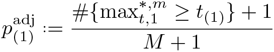
As was the case with the procedure of Holm (1979), this correction is a stepdown procedure: ĉ(1 − α, j) is weakly decreasing in j and, as such, the criterion for rejection is more demanding for more significant hypotheses and becomes less demanding for less significant hypotheses. Given that the null distributions based on $\max_{t, j}^{*, m}$ are based on resamples of the original data, they implicitly account for the underlying dependence structure of the test statistics, leading to potentially considerable gains in power over the Holm procedure, which assumes a worst-case dependence structure.

The above algorithm leads to a decision whether to reject or not reject for each null hypothesis H_s at a given significance level α. However, additionally and perhaps more conveniently, a multiple-testing-adjusted p-value can be directly computed for each H_s , as described in the algorithm below. This algorithm is a generalization of a resample-based p-value for a single null hypothesis, which can be defined as (Romano and Wolf 2016; Davison and Hinkley 1997, 158).

p : = \frac{# {t^{*, m} \geq t} + 1}{M + 1}

Note that other definitions exist.¹¹ To generalize this to a situation where multiple hypotheses are considered, rwolf implements the following algorithm to compute the p-values using the distribution of $\max_{t, j}^{*, m}$ , following Romano and Wolf (2016, algorithm 4.2).

p : = \frac{# {t^{*, m} \geq t}}{M}

Either option can be implemented in the rwolf command, as described in section 3.

Define

p_{(1)}^{adj} : = \frac{# {\max_{t, 1}^{*, m} \geq t_{(1)}} + 1}{M + 1}

For s = 2,…, S,

first let

p_{(s)}^{initial} : = \frac{# {\max_{t, s}^{*, m} \geq t_{(s)}} + 1}{M + 1}

and then enforce monotonicity by defining

p_{(s)}^{adj} : = \max {p_{(s)}^{initial}, p_{(s - 1)}^{adj}}

3 The rwolf command

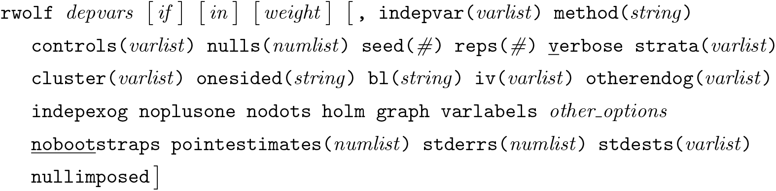
The Romano–Wolf multiple-hypothesis correction is implemented using the following syntax, returning the adjusted p-values described above, as well as the unadjusted p-values according to (6) [or (7), if noplusone is specified] for comparison.

where depvars refers to the multiple outcome variables that are being considered. There are two ways for this command to be used. First, indepvar() and method() must be specified if the complete Romano–Wolf procedure should be implemented including the estimation of bootstrap replications and generation of adjusted p-values. Alternatively, if the user is providing rwolf with precomputed bootstrap or permuted replications of the estimated statistic and standard errors for each of their multiple-hypothesis tests of interest, and only wishes for rwolf to calculate the adjusted p-values, then nobootstraps, pointestimates( numlist ), stderrs( numlist ), and stdests( varlist ) should be indicated. pweight s, aweight s, fweight s, and iweight s are allowed; see [U] 11.1.6 weight.

The first of these cases is provided for situations in which a single type of regression model is implemented with a range of outcome variables. In this case, rwolf can take care of the full procedure, including estimating the baseline models, and few details are required. The latter case is provided for more complex situations, such as cases where different models are used to test each hypothesis, where both dependent and independent variables change across models, or where more complicated resampling schemes are desired. Examples of each of these is provided in section 4.

3.1 Options

Standard options

indepvar( varlist ) indicates the independent (treatment) variable that is included in multiple-hypotheses tests. This will typically be a single independent variable; however, it is possible to indicate various independent (treatment) variables that are included in the same model. The Romano–Wolf procedure will be implemented, efficiently returning p-values for each dependent variable of interest, corresponding to each of the specified independent variables. This option must be specified unless the nobootstraps option is indicated (see below).

method( string ) indicates to Stata how each of the multiple-hypothesis tests (that is, the baseline models) are performed. Any standard regression–based estimation commands permitted by Stata may be specified, including logit, probit, ivregress, regress, and areg; see help estimation commands for a full list of estimation commands in Stata. The default is method(regress). If instrumental-variables (IV) estimation is desired, method() must be specified with ivregress only, and the iv() option below must be specified.

controls( varlist ) indicates additional controls that should be included in regressions of each depvar on the indepvar of interest. Any variable format accepted by varlist is permitted, including time series operators and factor variables.

nulls( numlist ) indicates the parameter values of interest (θ_s ⁰ in section 2.2) used in each test. A single scalar value should be indicated for each of the multiple hypotheses tested, and these values should be listed in the same order as the variables listed as depvars. If multiple indepvar() are specified, null parameters should be specified grouped first by indepvar() and then by depvars. For example, if two independent variables are considered with four dependent variables, first the four null parameters associated with the first independent variable should be listed, followed by the four null parameters associated with the second independent variable. By default, each null hypothesis is assumed to be that the parameter is equal to 0.

seed( # ) sets the seed to indicate the initial value for the pseudo-random-number generator. # may be any integer between 0 and 2³¹ − 1.

reps( # ) specifies to perform # bootstrap replications. The default is reps(100). Where possible, a larger number (by a magnitude) of replications should be used for more precise p-values. In IV models, a considerably larger number of replications is highly recommended.

verbose requests additional output, including display of the initial (uncorrected) models fit. This will also generate a summary output message indicating the number of hypotheses rejected in uncorrected models and when implementing the Romano–Wolf procedure, as well as any dependent variables for which the null is rejected in the Romano–Wolf procedure.

strata( varlist ) specifies the variables identifying strata. If strata() is specified, bootstrap samples are selected within each stratum when forming the resampled null distributions.

cluster( varlist ) specifies the variables identifying resampling clusters. If cluster() is specified, the sample drawn when forming the resampled null distributions is a bootstrap sample of clusters. This option should always be specified when underlying models require cluster–robust inference. cluster() does not cluster standard errors in each regression; if desired, this can be specified using vce(cluster clustvar ).

onesided( string ) specifies to calculate p-values based on one-sided tests. The default is p-values based on two-sided tests, corresponding to the null that each parameter is equal to 0 (or to the values indicated in nulls()). string must be either positive, in which case the null is that each parameter β ≥ 0, or negative, in which case the null is that each parameter β ≤ 0.

bl( string ) allows for the inclusion of baseline measures of the dependent variable as controls in each model. If desired, these variables should be created with some suffix, and the suffix should be included in the bl() option. For example, if outcome variables are called y1, y2, and y3, then variables y1_bl, y2_bl, and y3_bl could be created with baseline values, and bl(_bl) would be specified.

iv( varlist ) is only necessary when method(ivregress) is specified. The IVs for the treatment variable of interest should be specified in iv(). At least as many instruments as endogenous variables must be included.

otherendog( varlist ) specifies additional endogenous variables if more than one endogenous variable is required in ivregress models. By default, when the option method(ivregress) is specified, it is assumed that the variable specified in indepvar( varlist ) is an endogenous variable that must be instrumented. If this is the case, the variable should not be entered again in otherendog().

indepexog should be specified if method(ivregress) is specified but indepvar() is an exogenous variable. In this case, all endogenous variables must be specified in otherendog(), and all instruments must be specified in iv().

noplusone calculates the resampled and Romano–Wolf adjusted p-values without adding 1 to the numerator and denominator [that is, according to (7) rather than (6)].

nodots suppresses replication dots in bootstrap resamples.

holm specifies to provide p-values corresponding to the Holm (1979) correction along with the standard output. These will be included in the command output and stored in the final column of the matrix e(RW) (described in section 3.2 below).

graph requests that a graph be produced showing the Romano–Wolf null distribution corresponding to each variable examined. This graph shows the distribution of $\max_{t, j}^{*, m}$ from (5) for each j in 1,…, S. Examples of such a graph are provided in section 4.

varlabels specifies to name panels on the graph of null distributions using their variable labels rather than their variable names.

other_options are any additional options that correspond to the baseline regression model. All options permitted by the indicated method are allowed.

Options specific to cases where resampled estimates are user provided

nobootstraps indicates that no bootstrap replications be generated by the rwolf command. In this case, each variable indicated in depvars must consist of M bootstrap realizations of the statistic of interest corresponding to each of the multiple baseline models. Additionally, for each variable indicated in depvars, the corresponding standard errors for each of the M bootstrap replicates should be stored as another variable, and these variables should be indicated as stdests( varlist ). Finally, the original estimates corresponding to each model in the full sample should be provided in pointestimates( numlist ), and the original standard errors should be provided in stderrs( numlist ). nobootstraps may not be specified if indepvar() and method() are specified; for all standard implementations based on regression models, indepvar() and method() should be preferred.

pointestimates( numlist ) provides the estimated statistics of interest in the full sample corresponding to each of the depvars indicated in the command. These estimates must be provided in the same order as the depvars are specified. pointestimates() may not be specified if indepvar() and method() are specified; for all standard implementations based on regression models, indepvar() and method() should be preferred.

stderrs( numlist ) provides the estimated standard errors for each estimated statistic in the full sample. These estimates must be provided in the same order as the depvars are specified. stderrs() may not be specified if indepvar() and method() are specified; for all standard implementations based on regression models, indepvar() and method() should be preferred.

stdests( varlist ) contains variables consisting of estimated standard errors from each of the M resampled replications. These standard errors should correspond to the resampled estimates listed as each depvar and must be provided in the same order as the depvars are specified. stdests() may not be specified if indepvar() and method() are specified; for all standard implementations based on regression models, indepvar() and method() should be preferred.

nullimposed indicates that resamples are centered around the null rather than the original estimate. nullimposed is generally used only when permutations rather than bootstrap resamples are performed.

3.2 Stored results

rwolf is an e-class program and returns many elements in the e() list. It returns scalars corresponding to each calculated Romano–Wolf p-value, which are available as e(rw_ depvar ), where depvar refers to the name of each dependent variable. If multiple independent variables are considered, a scalar for each p-value corresponding to each independent–dependent variable pair will be returned as e(rw_ depvar_indepvar ). A matrix is also returned as e(RW) providing the full set of Romano–Wolf-corrected p-values. If the holm option is indicated, p-values according to Holm (1979) will be returned in column 4 of this matrix. Again if multiple independent variables are considered, a matrix named e(RW_ indepvar ) will be returned corresponding to each depvar.

4 Some examples

4.1 Regression-based examples and performance

We begin by presenting a particularly simple case. Consider the following linear model, in which 10 outcome variables y^s are regressed on a single independent variable, treat. Superscript-s terms refer to each of the multiple outcomes, of which there are a total of S, or their determinants. The data-generating process (DGP) is simulated as

y_{i}^{s} = β_{0}^{s} + β_{1}^{s} {treat}_{i} + ε_{i}^{s} for s = 1, \dots 10

for observation i. For each observation i, the 10 stochastic error terms $ε_{i}^{s}$ are drawn from a multivariate normal (mvn) distribution, following

ε_{i} ~ N ([\begin{array}{l} 0 \\ 0 \\ ⋮ \\ 0 \end{array}], [\begin{matrix} 1 & ρ & \dots & ρ \\ ρ & 1 & \dots & ρ \\ ⋮ & ⋮ & ⋱ & ⋮ \\ ρ & ρ & \dots & 1 \end{matrix}])

with ρ ≥ 0, and the independent variable of interest, treat _i , is generated as treat _i $1_{{U_{i} > 0.5}}$ , where 1 denotes the indicator function and U_i ∼ U(0, 1). This is a highly stylized setting, but it allows us to vary the correlation between the multiple outcome variables of interest (y ¹ , y ² ,…, y ¹⁰) via the parameter ρ, as well as the impact of treatment via the parameter $β_{1}^{s}$ . In particular, we can examine both the empirical fwer and the empirical proportion of false null hypotheses that get rejected (that is, power). We can examine this performance not only for the Romano–Wolf procedure but also for Holm’s procedure and for naïve procedures that do not account for multiple testing.

We consider a series of simulations based on N = 100 observations. Each null hypothesis is that $β_{1}^{s} = 0$ , versus the two-sided alternative hypothesis $β_{1}^{s} \neq 0$ . Across simulations, we vary the number of models in k = 1, 2,…, 10 for which $β_{1}^{s} = 0$ , as well as ρ, the correlation between outcomes induced by the stochastic error terms. Below, we document one such simulation and resulting multiple-hypothesis correction.

In the simulation below, each of the 10 $β_{1}^{s}$ terms is equal to 0, and the correlation between draws in the mvn distribution is set at ρ = 0.25. We follow the dgp described above, where first we simulate treat _i (as treat), and then we generate ε_i as a draw from an MVN. This draw is generated using a transformation of independent normal draws using a Cholesky decomposition of the desired covariance matrix and Stata’s matrix score command to multiply row vectors.¹²

Once we have simulated the N × S matrix Y in the above code, we apply the Romano–Wolf stepdown correction. Here we are considering the S = 10 outcome variables y1–y10 and the single independent variable treat. We request that the command perform 1,000 bootstrap repetitions, which, given the lack of other options, will be performed by resampling observational units with replacement. By specifying the nodots and holm options, we request that no dots be displayed on the Stata output to indicate the degree to which the resample procedure has advanced, and we request for rwolf to return p-values corrected using Holm’s (1979) procedure (which will be listed in the final column of tabular output and saved in the returned e() list).

The command returns a list of p-values associated with each of the multiple outcomes. The column Model p-value lists the analytical p-values coming directly from the estimated regression model based, in each case, on the t statistic and the (inverse) cumulative distribution function of a t distribution with appropriate degrees of freedom. The column Resample p-value lists the resampling-based p-values as per (6), which also do not correct for multiple testing. In the case of both of these uncorrected procedures, despite the fact that all true β ₁ values were 0, many of the hypotheses that β ₁ = 0 are rejected at α = 0.05. In particular, the variables y4 and y7 have p-values below 0.05 for both uncorrected procedures. The third column displays the Romano–Wolf adjusted p-values, where we note that now no null hypothesis is rejected (even at α = 0.10).

The simulated example above provides one example of a multiple-hypothesis correction based upon a known DGP. To examine the performance of the rwolf command (and the Romano–Wolf correction in this context) more generally, we can examine the error rates and proportion of hypotheses correctly rejected when we vary the number of values of β ₁ ^s = 0 and the correlation between outcomes, ρ. We consider such an example in tables 1 and 2 (which are in the spirit of tables 1–3 in Romano and Wolf [2005a]). The first table considers the proportion of times at least one null hypothesis is rejected when the null hypothesis is actually true (the FWER), and the second table considers the proportion of hypotheses that are correctly rejected when the null hypothesis is false (the power of the tests).¹³

In these tables, we consider 1) a series of models where all of the β ₁ ^s terms are equal to 0 (presented in panel A of table 1), 2) a series where half of the β ₁ ^s terms are equal to 0 and the other half are equal to 0.5 (presented in panel B of table 1 when considering FWERs and panel A of table 2 when considering power),¹⁴ and 3) a series where all of the β ₁ ^s terms are equal to 0.5 (presented in panel B of table 2). Case 1 is not considered in table 2 given that all null hypotheses are true and so cannot be “correctly rejected”. Similarly, case 3 is not considered in table 1 given that all null hypotheses are false and so the FWER is trivially equal to 0 given that they cannot be “incorrectly rejected”. Across columns, we vary the degree of correlation between outcomes, from ρ = 0 in the first two columns, to ρ = 0.75 in the final two columns. The nominal levels for the FWER are set at α = 0.05 and α = 0.10, respectively.

Table 1.

Simulated error rates

	ρ = 0		ρ = 0.25		ρ = 0.50		ρ = 0.75
	5%	10%	5%	10%	5%	10%	5%	10%
Panel A: All β ₁=0
FWER uncorrected	0.396	0.642	0.365	0.602	0.281	0.492	0.197	0.341
FWER Holm	0.035	0.094	0.036	0.084	0.029	0.068	0.021	0.046
FWER Romano–Wolf	0.048	0.100	0.049	0.097	0.046	0.097	0.047	0.096
Panel B: Half β ₁=0.5
FWER uncorrected	0.222	0.408	0.212	0.390	0.180	0.335	0.147	0.258
FWER Holm	0.024	0.065	0.028	0.061	0.025	0.052	0.025	0.049
FWER Romano–Wolf	0.029	0.067	0.033	0.067	0.034	0.075	0.040	0.083

notes: Error rates are documented familywise over all outcomes. Uncorrected error rates are displayed at the top of each panel, where the proportion refers to the proportion of simulations where at least one true null hypothesis was falsely rejected. Below, similar rates are displayed when p-values are corrected using Holm’s and Romano–Wolf’s procedures. The correlation between outcomes is varied across columns, and error rates at α = 0.05 and α = 0.10 are displayed. The number of repetitions is 1,000 per scenario, and the number of bootstrap resamples in each case is equal to M = 5000.

Table 2.

Simulated rejection rates

	ρ = 0		ρ = 0.25		ρ = 0.50		ρ = 0.75
	5%	10%	5%	10%	5%	10%	5%	10%
Panel A: Half β ₁=0.5
Rejected uncorrected	0.687	0.791	0.689	0.797	0.681	0.789	0.693	0.798
Rejected Holm	0.324	0.460	0.325	0.457	0.325	0.453	0.340	0.468
Rejected R–W	0.373	0.486	0.382	0.492	0.401	0.519	0.469	0.594
Panel B: All β ₁=0.5
Rejected uncorrected	0.683	0.792	0.689	0.794	0.681	0.788	0.694	0.797
Rejected Holm	0.384	0.547	0.406	0.558	0.409	0.552	0.432	0.564
Rejected R–W	0.416	0.558	0.436	0.576	0.458	0.593	0.519	0.651

notes: The rate of correctly rejected (false) null hypotheses is displayed, where rates refer to the proportion of all hypotheses rejected across all simulations where the null hypothesis is false. “Uncorrected” rejection rates are for cases where naïve p-values are used for each test, “Holm” rejection rates are based on Holm’s p-value correction, and “R–W” rates are based on Romano–Wolf’s p-value correction. The correlation between outcomes is varied across columns, and rejection rates at α = 0.05 and α = 0.10 are displayed. The number of repetitions is 1,000 per scenario, and the number of bootstrap resamples in each case is equal to M = 5000.

Here we briefly discuss the performance of the rwolf command and note several important features of the Romano–Wolf multiple-hypothesis correction. In particular, we always present the performance criteria for three testing procedures: those corresponding to the naïve case, where no correction for multiple-hypothesis testing is made; those corresponding to Holm’s procedure; and those corresponding to the Romano–Wolf procedure.

In panel A of table 1 (where all values for $β_{1}^{s} = 0$ ), it is clear in the uncorrected case that the empirical FWERs greatly exceed nominal levels of α = 0.05 and 0.10. When all outcomes are uncorrelated, these values are 0.396 and 0.642, respectively, suggesting a large proportion of families in which a null hypothesis is incorrectly rejected, in line with that predicted in theory.¹⁵ As the correlation between outcomes grows, these naïve values fall closer to the nominal levels but still considerably exceed desired error rates.

With the Holm correction, we observe that the FWER is controlled at both the 5% and 10% levels. This is observed regardless of the degree of correlation considered, between ρ = 0 and ρ = 0.75. Similar control is observed with the Romano–Wolf procedure. Indeed, in each case the empirical FWER is very close to the desired nominal rate of 0.05 or 0.10, respectively. In panel B of table 1 (where 5 of the 10 hypotheses should not be rejected), we again observe that the FWER without multiple-hypothesis correction still substantially exceeds desired error rates but is successfully controlled at no more than α with both the Holm and Romano–Wolf procedures.

In table 2, we can examine the relative power of the Holm and Romano–Wolf procedures for rejecting false null hypotheses. In panel A of table 2, we return to the case considered in panel B of table 1, here considering the power of the tests instead. In this setting, the naïve case of no multiple-hypothesis correction allows us to reject a large proportion of false null hypotheses (at the cost of the FWER documented in table 1).

In the case of Holm and Romano–Wolf, we observe relatively similar rates of correct rejection when the correlation between outcomes is 0, but as expected, as the correlation between outcomes grows, the Romano–Wolf procedure substantially improves relative to Holm’s procedure. For example, in the final column of panel A, we reject 59.4% of false null hypotheses using the Romano–Wolf procedure versus only 46.8% using Holm’s procedure, a 27% improvement in rejection rate. A similar pattern is observed in table 2, panel B (where all null hypotheses are false). Initially, when the correlation between outcomes is 0, Holm’s and Romano–Wolf’s procedures have similar power; however, to the degree that ρ increases, the Romano–Wolf procedure becomes relatively more powerful.

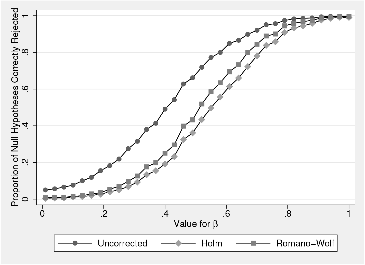
In table 2, we consider the relative power of testing procedures for rejecting false null hypotheses with a particular value for β ₁ ^s , in this case, $β_{1}^{s} = 0.5$ for all cases where $β_{1}^{s} \neq 0$ . The relative power of these procedures will depend on the actual value of β ₁ ^s . Below, in figure 1, we consider how these rates of rejection vary with $β_{1}^{s}$ values. In the figure, we consider the case corresponding to table 2 panel B (where all $β_{1}^{s} \neq 0$ ) and where ρ = 0.5. We present values of $β_{1}^{s}$ varying from 0.01 to 1, in steps of 0.03. All other details follow the DGP in (8).

Figure 1.

Comparative power to reject false null hypotheses. notes: For each value of β ₁ in {0.01, 0.04, 0.07,…, 0.97, 1}, we conduct 1,000 simulations following the DGP laid out in (8), where each β ₁ ^s is set to the value indicated on the x axis and ρ = 0.5. In each case, N = 100 observations are simulated, and we calculate p-values using the rwolf command with 200 bootstrap resamples.

For each value of β ₁, we run 1,000 simulations, in each case calculating the unadjusted p-values, and the Holm and Romano–Wolf p-values using the rwolf command. Across the 1,000 simulations, we examine the proportion of null hypotheses correctly rejected. As expected, the power when not conducting any multiple-hypothesis correction is greatest (at the cost of exceeding the FWER if the null hypothesis were true). To the degree that the correlation between outcomes approaches ρ = 1, the power of the Romano–Wolf procedure will approach the power of the procedure with no multiplehypothesis correction.

Of interest is the relative performance of Romano–Wolf’s versus Holm’s correction. Here, given that ρ = 0.5, the power of the Romano–Wolf correction dominates the power of the Holm correction across each value for β ₁. This difference is particularly notable at values of β ₁ between 0.4 and 0.6, and all disappear as β ₁ becomes large, implying sufficient power to reject all null hypotheses regardless of the correction procedure. When β ₁ = 1, each of the procedures results in rejection rates of around 100%.

The simulated examples based on rwolf displayed previously provide a standard implementation where multiple outcome variables are regressed on a single independent (treatment) variable, each using an ordinary least-squares regression. However, the standard command syntax of rwolf allows for many extensions of this baseline implementation. This includes the use of alternative estimation methods (for example, IV regression, probit, and other Stata estimation commands), the implementation of one-sided tests, or the use of alternative bootstrap routines (for example, block and stratified bootstraps). To document several such extensions, we turn to an alternative example below, modeled after a simple IV regression example based on system data, as described in the help file of Stata’s ivregress. Here we extend to a case with multiple outcomes and examine both a one- and a two-sided test.

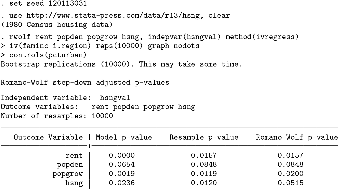
We begin with a (default) two-sided test, where we follow the implementation of the two-stage least-squares estimate from the ivregress help file.¹⁶ We use the same specification, where along with the outcome variable rent, we also consider three other variables: popden, popgrow and hsng. We do not make any claim to causality or consistency of the resulting estimates. These are simply shown as an illustration of the rwolf command with an IV regression. In each case, the independent variable of interest is hsngval, and this is instrumented with the variables indicated in the iv() option. We include pcturban as an additional control. We use 10,000 bootstrap replications (bootstrapping on observational units) and request a graph of the null distributions used in testing be reported (as discussed below).

The setup and output of this Romano–Wolf correction is displayed below. In this example, the p-values from the original IV models are quite low, suggesting evidence against the null that each coefficient on the variable hsngval is 0. The Romano–Wolf correction displayed in the final column results in inflated p-values (as designed), though the adjusted p-values are still relatively low.

Below, we document the same procedure but here conducting one-sided hypothesis tests. In each case, the null hypothesis in these tests will be of the form H ₀ : β ₁ ≤ 0, versus the alternative H ₁ : β ₁ > 0, where β ₁ is the coefficient on hsngval in the second stage of the IV regression. For the sake of illustration, we multiply the two outcomes by −1, such that the sign on ${\hat{β}}_{1}$ estimated in each IV regression is greater than 0. Along with the syntax described previously, the implementation of one-sided tests requires the use of the option onesided(). If onesided(negative) is specified, the null will be H ₀ : β ₁ ≤ 0; that is, negative values will provide more support for the null. On the other hand, if onesided(positive) is specified, the null will be H ₀ : β ₁ ≥ 0 in each case, such that positive values will provide more support for the null.

In each example, we specified the graph option to request as output the null distributions used to calculate the p-value in each case. Examining these distributions allows us to empirically observe how much more demanding the Romano–Wolf correction is compared with an uncorrected test.

In figure 2 panel (a), we display these distributions in the two-sided case. Here the histogram presents the absolute value of each (Studentized) estimate from the bootstrap replications where the null is imposed, and the black dotted line presents an exact half-normal distribution. The actual Studentized value of the regression coefficient is displayed as a solid vertical line. In the top left panel, the first null distribution is considerably more demanding than the theoretical distribution, given that it accumulates the maximum coefficient estimated across each outcome. These null distributions become increasingly less demanding in the top right and bottom left panels because previously tested variables are removed from the pool to form the null distributions. Finally, in the bottom right corner (for the least significant variable), the null distribution is based on bootstrap replications from only this variable, and as such, the null distribution closely approximates the theoretical half-normal distribution.

Figure 2.

Null distributions for one- and two-sided tests with IV models. notes: Panel (a) documents the null distributions used to calculate the Romano–Wolf adjusted p-values for each of the four outcome variables of interest in the ivregress command, using a two-tailed test where the null is that β ₁ = 0 in each case. Panel (b) documents the null distributions for the same regressions but now based on the one-tailed test where each null is that β ₁ ≤ 0.

In figure 2 panel (b), we present the same null distributions but now based on the one-sided tests. Here the histogram documents the maximum values across the multiple variables in each bootstrap replication, and the black dotted line presents the theoretical normal distribution. Once again, when we consider outcomes for which more significant relationships are observed, the empirical distribution used to calculate the corrected p-value is considerably more demanding than the black dotted distribution, which would be used under no correction and a normality assumption. In the case of the least significant variable (popden), these two distributions are similar given that the null distribution is based only on Studentized regression estimates of the single regression where this is the outcome variable.

4.2 A nonstandard Studentized example

Each previous example has been based on the simple rwolf command syntax where a single independent variable is regressed on multiple outcome variables. This is frequently sufficient for a large number of implementations, such as cases where a single experimental treatment is assigned, and various outcomes are measured. In this case, the rwolf command can be implemented in one line and takes care of everything, including the full process of bootstrap draws, estimation of regression coefficients and standard errors, as well as the generation of null distributions and p-values. However, Romano–Wolf p-values can also be calculated for more complex setups, if the user wishes to pass the command the already-bootstrapped (or permuted) statistics and standard errors that have been calculated from the underlying models of interest. We document this flexibility in what remains of this section, using a bootstrap approach where our statistics of interest are a series of correlations.

We use an example and data documented in Westfall and Young (1993), which was also previously used to demonstrate the effectiveness of the Romano–Wolf procedure in Romano and Wolf (2005a). Although we refer to this as a nonstandard example, it is only nonstandard in the way it interacts with the syntax of rwolf, given that the multiple tests are based on several independent variables and as such do not allow for a single independent variable to be indicated using the indepvar() option.

This example considers pairwise correlations between state-average standardized Scholastic Aptitude Test (SAT) scores and several other state-level measures for the 48 mainland U.S. states plus Hawaii. These data—consisting simply of state-level measures of several variables of interest—are provided in table 6.4 of Westfall and Young (1993, 197) as well as in the replication materials for this article. The variables considered are satdev (the residuals from a regression of state-level SAT scores on the square root of the percent of students taking the exam in a given state), the student/teacher ratio in the state, the teacher salary, the percent of the population that is black, and the crime rate of each state.

In this case, the statistics of interest refer to simple correlations between pairs of variables of interest, and p-values will be corrected for the fact that we are testing 10 hypotheses. To construct null distributions following (4) and (5), the rwolf command requires an estimate of the original parameter of interest in each case (the pairwise correlation) along with a standard error. These values are used to construct t_s (as defined in section 2.2) for each of the s multiple hypotheses and to order the hypotheses in terms of their relative significance. The command additionally requires the results from M bootstrap replicates, where a resampled estimate of each statistic and its standard error is provided. We document such a case below, where in each of the multiple hypotheses the parameter of interest is the correlation between variables ρ (which can be simply calculated using corr in Stata) and its standard error, which, assuming normality, is calculated as (Bowley 1928; Zar 2010)¹⁷

{SE}_{\hat{ρ}} : = \sqrt{\frac{1 - {\hat{ρ}}^{2}}{N - 2}}

To generate the various components that rwolf uses to implement the multiplehypothesis correction, we first open the data and define in locals var1 and var2 the corresponding pairs to be tested. The idea in these locals is that we wish to calculate the correlation between the first variable listed in var1 and the first variable listed in var2, the correlation between the second variable listed in var1 and the second variable listed in var2, and so forth, through the correlation between the last variable listed in var1 and the last variable listed in var2. We calculate these correlations one by one in the foreach loop in the code below. We loop over elements of the local var1, and we take corresponding elements one by one from local var2 using Stata’s tokenize command.¹⁸ These correlations and standard errors from the original data are then saved, respectively, as locals c’i’ and s’i’ to be later passed to the rwolf command. Finally, we generate two series of 10 empty variables, rho1–rho10 and std1–std10, which will later be populated by resample-based correlation estimates and their standard errors.

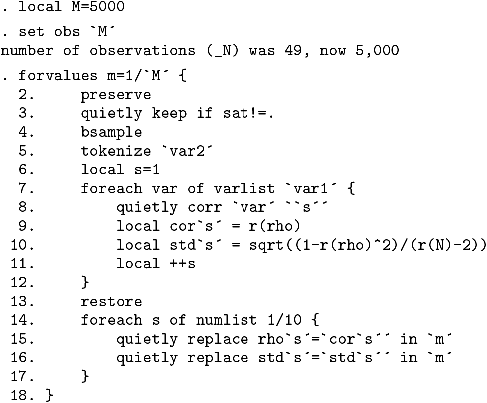
A bootstrap procedure is then implemented based on 5,000 resamples. We initially expand the dataset to have 5,000 observations to store each of the bootstrap estimates; however, prior to calculating the correlations and standard errors in each replicate, we work only with the 49 state-level observations with SAT data. Each replicate is implemented in the main forvalues loop below. Within each of these 5,000 iterations, we first issue a preserve command to later restore the data toward the end of each iteration; this way, the bootstrap resample (bsample) begins with the original data in each iteration. Within each loop, lines 7–12 calculate the bootstrap correlations and corresponding standard errors, which are then filled in line by line in the variables rho1–rho10 and std1–std10 at the end of each loop.

Once we have stored the original estimates plus their standard errors and have variables containing resampled estimates along with their resampled standard errors, we can simply request the multiple-hypothesis correction from rwolf, as laid out in section 3. This is implemented below.

We pass to rwolf the varlist consisting of resampled estimates. The stdests( varlist ) option consists of bootstrap standard errors. Finally, the original correlations and standard errors from the (original) data are passed as numlists in pointestimates() and stderrs(). The graph option requests that a graph be produced documenting the null distributions used in each test, and noplusone requests that the p-value be calculated following (7) rather than the standard (6).

In this nonstandard implementation, no Model p-value is returned because rwolf itself does not estimate the original correlations, simply working with the estimates provided from the above code. In this case, we observe the Resample p-value (which is not corrected for multiple-hypothesis testing), which is the results of comparing each original estimate with the null distribution, and the Romano-Wolf p-value, where the multiple-hypothesis correction has been implemented as indicated in section 2.2. These results are similar to those observed in Romano and Wolf (2005a, table 4) and would result in rejecting the same hypotheses if standard cutoffs (such as α = 0.01, α = 0.05, or α = 0.10) were used.

In figure 3, we present the graph of null distributions, based on (5), for each hypothesis. As implied by the multiple-hypothesis testing algorithm, the null distributions become less demanding while moving from the most significant variable (top left-hand panel) to the least significant variable (left-hand panel in the final row).

Figure 3.

Null distributions and original t statistics from the SAT-deviation data. notes: Each panel documents the null distributions used to calculate the Romano–Wolf adjusted p-values [following (5)] for each of the 10 outcome variables of interest. The histogram in each panel plots the stepdown resampled null distribution, the dashed line represents the theoretical half-normal, and the solid vertical line represents the original t statistic corresponding to each correlation.

5 Conclusions

In this article, we described the Romano–Wolf multiple-hypothesis correction, a flexible and versatile procedure to (asymptotically) control the FWER when testing a family of hypotheses at the same time, which occurs frequently in applied work in economics, finance, and many other fields. The article documented the rwolf command, which returns (multiple-testing) adjusted p-values that a) do not suffer from inflated rates of type I error and b) take into account the dependence structure of test statistics via resampling. The latter feature, together with the stepwise nature of the procedure, results in improved ability to correctly reject false null hypotheses (that is, power) compared with more traditional multiple-testing procedures, such as the Bonferroni procedure and the Holm procedure.

We documented the syntax of the command and provided several illustrative examples, with both simulated data and real data. We documented how this command can be easily used in cases where multiple dependent variables are regressed on a single independent variable (in a broad class of regression models). In this case, implementing the Romano–Wolf multiple-hypothesis correction in Stata is a one-line endeavor, because the command interacts directly with Stata’s estimation commands to implement the p-value adjustment. We also documented a more complex case, where the statistics of interest are not based on regression models and where multiple independent variables are also considered.

We envision this code being used in a variety of circumstances where multiplehypothesis testing occurs, avoiding the well-known and undesirable pitfalls of the phenomenon interchangeably called “data mining”, “cherry picking”, or “p-hacking”.

Supplemental Material

Supplemental Material, st0618 - The Romano–Wolf multiple-hypothesis correction in Stata

Supplemental Material, st0618 for The Romano–Wolf multiple-hypothesis correction in Stata by Damian Clarke, Joseph P. Romano and Michael Wolf in The Stata Journal

Footnotes

6 Programs and supplemental materials

To install a snapshot of the corresponding software files as they existed at the time of publication of this article, type

Notes

A Westfall and Young’s “Free Stepdown Resampling Method”

For background related to the multiple-hypothesis testing procedures discussed in section 2 of this article, we describe the stepdown resampling procedure of Westfall and Young (1993) here. This procedure is described as algorithm 2.8 in , 66–67), and we largely follow their notation but adapt it to fit the notation laid out in section 2 of this article.

This procedure begins with S multiple hypotheses, each associated with its own (unadjusted) p-value. These p-values are labeled such that p ₁ ≤ p ₂ ≤ · · · ≤ p_S . It then proceeds as described below.

Begin with a counter, COUNT _s = 0 for each s = 1,…, S.

Using a bootstrap sample, generate a vector of analogous p-values,. $(p_{1}^{*}, p_{2}^{*}, \dots, p_{S}^{*})$ . These will not necessarily follow the same ordering as the original p-values.

Define the successive minimums:

\begin{matrix} q_{S}^{*} = p_{S}^{*} \\ q_{S - 1}^{*} = \min (q_{S}^{*}, p_{S - 1}^{*}) \\ q_{S - 2}^{*} = \min (q_{S - 1}^{*}, p_{S - 2}^{*}) \\ ⋮ \\ q_{1}^{*} = \min (q_{2}^{*}, p_{1}^{*}) \end{matrix}

If $q_{s}^{*} < p_{s}$ , then increment COUNT _s by one unit.

Repeat steps 2–4 N times, and compute $\tilde{p}$ _s = COUNT _s /N.

Enforce monotonicity using successive maximization:

\begin{matrix} p_{WY,1}^{adj} = {\tilde{p}}_{1} \\ p_{WY,2}^{adj} = \max (p_{WY,1}^{adj}, {\tilde{p}}_{2}) \\ ⋮ \\ p_{WY, S}^{adj} = \max (p_{WY, S - 1}^{adj}, {\tilde{p}}_{S}) \end{matrix}

The adjusted p-values $(p_{WY,1}^{adj}, p_{WY,2}^{adj}, \dots p_{WY, S}^{adj})$ in the vector are the p-values corrected for multiple-hypothesis testing, where subscript WY refers to the Westfall–Young procedure. These p-values provide strong control of the FWER under the assumption of subset pivotality.

B Regression-based examples

Below, we replicate the example from section 4.2, except that here we estimate the regressions rather than calculating correlations directly (see, for example, line 2 of the first loop, and line 8 of the final principal loop). Given that t statistics calculated from each regression are identical to those calculated using the estimate of the correlation and its standard error in (9), the Studentization can be similarly performed by regression. This is documented below, where, apart from the regressions themselves, all other details follow those described in section 4.2.

References

Anderson

M. L.

2008. Multiple inference and gender differences in the effects of early intervention: A reevaluation of the Abecedarian, Perry Preschool, and Early Training Projects. Journal of the American Statistical Association 103: 1481–1495. https://doi.org/10.1198/016214508000000841.

Attanasio

O. P.

Fern´andez

Fitzsimons

E. O. A.

Grantham-McGregor

S. M.

Meghir

Rubio-Codina

. 2014. Using the infrastructure of a conditional cash transfer program to deliver a scalable integrated early child development program in Colombia: Cluster randomized controlled trial. British Medical Journal 349: g5785. https://doi.org/10.1136/bmj.g5785.

Benjamini

Hochberg

. 1995. Controlling the false discovery rate: A practical and powerful approach to multiple testing. Journal of the Royal Statistical Society, Series B 57: 289–300. https://doi.org/10.1111/j.2517-6161.1995.tb02031.x.

Bonferroni

C. E.

1935. Il calcolo delle assicurazioni su gruppi di teste. In Studi in Onore del Professore Salvatore Ortu Carboni, 13–60. Rome: Tipografia del Senato.

Bowley

A. L.

1928. The standard deviation of the correlation coefficient. Journal of the American Statistical Association 23: 31–34. https://doi.org/10.2307/2277400.

Clarke

2016. rwolf: Stata module to calculate Romano–Wolf stepdown p-values for multiple hypothesis testing. Statistical Software Components S458276, Department of Economics, Boston College. https://ideas.repec.org/c/boc/bocode/s458276.html.

Davison

A. C.

Hinkley

D. V.

. 1997. Bootstrap Methods and Their Application. Cambridge: Cambridge University Press.

DiCiccio

C. J.

Romano

J. P.

. 2017. Robust permutation tests for correlation and regression coefficients. Journal of the American Statistical Association 112: 1211–1220. https://doi.org/10.1080/01621459.2016.1202117.

Efron

1979. Bootstrap methods: Another look at the jackknife. Annals of Statistics 7: 1–26. https://doi.org/10.1214/aos/1176344552.

10.

Gertler

Heckman

Pinto

Zanolini

Vermeersch

Walker

Chang

S. M.

Grantham-McGregor

. 2014. Labor market returns to an early childhood stimulation intervention in Jamaica. Science 344: 998–1001. https://doi.org/10.1126/science.1251178.

11.

Gould

1995. FAQ: Stata 6: Simulating multivariate normal observations. https://www.stata.com/support/faqs/statistics/multivariate-normal-observations/.

12.

Holm

1979. A simple sequentially rejective multiple test procedure. Scandinavian Journal of Statistics 6: 65–70.

13.

Jones

Molitor

Reif

. 2019. What do workplace wellness programs do? Evidence from the Illinois Workplace Wellness Study. Quarterly Journal of Economics 134: 1747–1791. https://doi.org/10.1093/qje/qjz023.

14.

Lehmann

E. L.

Romano

J. P.

. 2005a. Testing Statistical Hypotheses. 3rd ed. New York: Springer.

15.

Lehmann

E. L.

Romano

J. P.

. 2005b. Generalizations of the familywise error rate. Annals of Statistics 33: 1138–1154. https://doi.org/10.1214/009053605000000084.

16.

List

J. A.

Shaikh

A. M.

. 2019. Multiple hypothesis testing in experimental economics. Experimental Economics 22: 773–793. https://doi.org/10.1007/s10683-018-09597-5.

17.

Liu

L. Y.

Patton

A. J.

Sheppard

. 2015. Does anything beat 5-minute RV? A comparison of realized measures across multiple asset classes. Journal of Econometrics 187: 293–311. https://doi.org/10.1016/j.jeconom.2015.02.008.

18.

Newson

R. B.

2010. Frequentist q-values for multiple-test procedures. Stata Journal 10: 568–584. https://doi.org/10.1177/1536867X1101000403.

19.

Newson

R. B.

, and the ALSPAC Study Team. 2003. Multiple-test procedures and smile plots. Stata Journal 3: 109–132. https://doi.org/10.1177/1536867X0300300202.

20.

Reif

2017. wyoung: Stata module to perform multiple testing corrections. Statistical Software Components S458440, Department of Economics, Boston College. https://ideas.repec.org/c/boc/bocode/s458440.html.

21.

Romano

J. P.

Shaikh

A. M.

Wolf

. 2010. Hypothesis testing in econometrics. Annual Review of Economics 2: 75–104. https://doi.org/10.1146/annurev.economics.102308.124342.

22.

Romano

J. P.

Wolf

. 2005a. Exact and approximate stepdown methods for multiple hypothesis testing. Journal of the American Statistical Association 100: 94–108. https://doi.org/10.1198/016214504000000539.

23.

Romano

J. P.

Wolf

. 2005b. Stepwise multiple testing as formalized data snooping. Econometrica 73: 1237–1282. https://doi.org/10.1111/j.1468-0262.2005.00615.x.

24.

Romano

J. P.

Wolf

. 2016. Efficient computation of adjusted p-values for resampling-based stepdown multiple testing. Statistics & Probability Letters 113: 38–40. https://doi.org/10.1016/j.spl.2016.02.012.

25.

Westfall

P. H.

Young

S. S.

. 1993. Resampling-Based Multiple Testing: Examples and Methods for p-Value Adjustment. New York: Wiley.

26.

Zar

J. H.

2010. Biostatistical Analysis. 5th ed. New York: Pearson.

Supplementary Material

Please find the following supplemental material available below.

For Open Access articles published under a Creative Commons License, all supplemental material carries the same license as the article it is associated with.

For non-Open Access articles published, all supplemental material carries a non-exclusive license, and permission requests for re-use of supplemental material or any part of supplemental material shall be sent directly to the copyright owner as specified in the copyright notice associated with the article.

0.00 MB