Sage Journals: Discover world-class research

Abstract

In this article, we describe jackknife2, a new prefix command for jackknifing linear estimators. It takes full advantage of the available leave-one-out formula, thereby allowing for substantial reduction in computing time. Of special note is that jackknife2 allows the user to compute cross-validation and diagnostic measures that are currently not available after ivregress 2sls, xtreg, and xtivregress.

Keywords

st0617 jackknife2 jackknife heteroskedasticity-consistent standard errors cross-validation diagnostic checking predictive residuals

1 Introduction

The jackknife (Quenouille 1956; Tukey 1958; Miller 1974; Efron 1982) is a method for assessing the accuracy of an estimator from data that are independently and identically distributed (i.i.d.) but not necessarily conditionally homoskedastic. Its basic idea is to exploit the information contained in the empirical distribution of the estimates computed from the n subsamples of size n − 1 that can be obtained from a sample of size n by leaving out one data point at a time. The jackknife is known to work very well for linear estimators, such as ordinary least-squares (OLS) and instrumentalvariables (IV) estimators, which are the workhorses of empirical research in a variety of fields. For these estimators, the jackknife may be implemented using simple formula for the effect of leaving out either one data point or one block of data points at a time. These leave-one-out (L1O) formula also represent the basis for other methods, including cross-validation (CV) procedures for model selection (Stone 1974, 1977) and diagnostic procedures for detecting heteroskedasticity, influential observations, and high-leverage points (Cook and Weisberg 1982).

The current Stata implementation of the jackknife is very general because it applies to both linear and nonlinear estimators. However, this generality comes at a cost in terms of computational speed when linear estimators are considered. For example, if one types regress yvar xvar , vce(jackknife), Stata computes the jackknife estimate of the sampling variance of the OLS estimator by literally leaving out one observation at a time and then recomputing the OLS estimates for each of the n subsamples of n − 1 observations. The same is true when using the vce(jackknife) option for the IV command ivregress or the panel versions of the OLS and IV commands, xtreg and xtivregress, or when using the jackknife prefix command for statistics that are linear in the data. With “big data” (either a large sample size or many regressors), this way of implementing the jackknife causes unnecessarily long computing times and therefore restricts the applicability of the method to samples with at most a few thousand observations.

In this article, we introduce a new procedure for jackknifing linear estimators. Our procedure takes full advantage of the available L1O formula, thereby achieving substantial reductions in computing time. Because postestimation commands that implement CV and diagnostic procedures are currently available only after regress, we also extend these commands to ivregress 2sls, xtreg, and xtivregress. We hope that this will help promote a wider application of the jackknife and related methods in empirical research.

2 The basic L1O formula

This section presents the basic L1O formula for OLS and IV estimators, both for crosssectional and panel data. The following sections then show how these formulas may be used for inference (section 3), model selection (section 4), and diagnostic checking (section 5).

2.1 Cross-sectional data

Let the random variable Y and the random vector X represent, respectively, the outcome of interest and a set of k regressors (including the constant term). We denote by Y the n-vector containing the observations on Y and by X the n × k matrix containing the observations on X. We assume that X has full column rank k < n. We also denote by Y_i the ith element of Y and by $X_{i}^{⊤}$ the ith row of X. Our parameter of interest is the unknown k-vector β in the linear model Y = Xβ + U, where U is an n-vector of unobservable regression errors.

OLS estimation

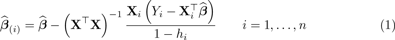
If there are no endogeneity problems, that is, the regressors are uncorrelated with the regression errors, an OLS regression of Y on X provides the standard way of estimating β . The OLS estimate of β computed from the full sample is $\hat{β} = {(X^{⊤} X)}^{- 1} X^{⊤} Y$ , while the estimate computed by excluding the ith data point $(X_{i}^{⊤}, Y_{i})$ is

{\hat{β}}_{(i)} = \hat{β} - {(X^{⊤} X)}^{- 1} \frac{X_{i} (Y_{i} - X_{i}^{⊤} \hat{β})}{1 - h_{i}} i = 1, \dots, n

where h_i is the ith diagonal element of the “hat” matrix H = X(X ^⊤ X)⁻ ¹ X ^⊤ (see, for example, Peracchi [2001]). Because H is a projection matrix (that is, symmetric and idempotent), 0 ≤ h_i ≤ 1. The k-vector $n (\hat{β} - {\hat{β}}_{(i)})$ , viewed as a function of i = 1,…, n, is called the sensitivity curve or empirical influence function (EIF) of OLS. The ith data point is said to be influential if the difference $\hat{β} - {\hat{β}}_{(i)}$ is large in some norm. Notice that the influence of the ith data point on the OLS coefficient depends on both $\hat{U}$ _i and h_i . If h_i is near one, then the ith data point is said to exert a high leverage.

IV estimation

If there are endogeneity problems, that is, the regressors are correlated with the regression errors, the available data on Y and X are generally insufficient to estimate β consistently. In this case, the IV method offers a solution provided one can find a set of r ≥ k valid instruments, namely, variables that are both exogenous (that is, uncorrelated with the regression errors) and relevant (that is, correlated with the regressors). We denote by W the n × r matrix containing the n observations on the r instruments and by $W_{i}^{⊤}$ the ith row of W. We also assume that the matrix W ^⊤ X has full column rank k ≤ r.

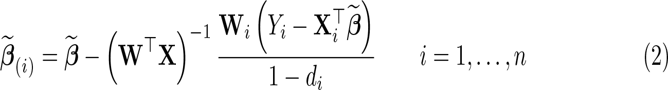
With r = k instruments (the “exactly identified” case), the IV estimator of β is unique and is called a simple IV estimator. The simple IV estimate computed from the full sample is $\tilde{β} = {(W^{⊤} X)}^{- 1} W^{⊤} Y$ , while the estimate computed by excluding the ith data point $(X_{i}^{⊤}, W_{i}^{⊤}, Y_{i})$ is

{\tilde{β}}_{(i)} = \tilde{β} - {(W^{⊤} X)}^{- 1} \frac{W_{i} (Y_{i} - X_{i}^{⊤} \tilde{β})}{1 - d_{i}} i = 1, \dots, n

where $d_{i} = X_{i}^{⊤} {(W^{⊤} X)}^{- 1} W_{i}$ is the ith diagonal element of the matrix X(W ^⊤ X)⁻ ¹ W ^⊤.

With r > k instruments (the “overidentified” case), the number of IV estimators is infinite. By far the most popular among them is the two-stage least-squares (2sls) estimator. The estimate computed from the full sample is $\tilde{β} = {(X^{⊤} C X)}^{- 1} X^{⊤} C Y$ , where C = W(W ^⊤ W)⁻ ¹ W ^⊤ is an n × n matrix. Phillips (1977) showed that the estimate computed by excluding the ith data point is

{\tilde{β}}_{(i)} = \tilde{β} - P^{- 1} R_{i} i = 1, \dots, n

with

\begin{matrix} P = X^{⊤} C X \\ R_{i} = J_{i} {(Y_{i} - {\hat{X_{i}}}^{⊤} \tilde{β}) - (Y_{i} - W_{i}^{⊤} \hat{π}) - (J_{i} + K_{i}) (Y_{i} - X_{i}^{⊤} \tilde{β})} \\ J_{i} = \frac{m_{i}}{e_{i} f_{i}} {\hat{V}}_{i} + \frac{{\hat{V}}_{i}^{⊤} P^{- 1} X_{i}}{e_{i} f_{i}} X_{i} \\ K_{i} = \frac{{\hat{V}}_{i}^{⊤} P^{- 1} X_{i}}{e_{i} f_{i}} {\hat{V}}_{i} - \frac{1}{e_{i}} X_{i} \\ e_{i} = m_{i} + \frac{{({\hat{V}}_{i}^{⊤} P^{- 1} X_{i})}^{2}}{f_{i}} \\ f_{i} = 1 - c_{i} + {\hat{V}}_{i}^{⊤} P^{- 1} {\hat{V}}_{i} \end{matrix}

where $\hat{π} = {(W^{⊤} W)}^{- 1} W^{⊤} Y$ is the r-vector of coefficients from the “reduced-form” ols regression of Y on the instruments in $W, \hat{X_{i}} = X^{⊤} W {(W^{⊤} W)}^{- 1} W_{i}$ and ${\hat{V}}_{i} = X_{i} - {\hat{X}}_{i}$ are the k-vectors of fitted values and residuals for the ith unit from the “first-stage” OLS regressions of the k variables in X on the r instruments in W, and $m_{i} = 1 - X_{i}^{⊤} P^{- 1} X_{i}$ and $c_{i} = W_{i} {(W^{⊤} W)}^{- 1} W_{i}^{⊤}$ are the ith diagonal elements of the matrices M = I _n − XP ⁻ ¹ X ^⊤ and C.

2.2 Panel data

To simplify the notation and with little loss of generality, let us consider a balanced panel dataset in which n units are all observed at the same T time points. Our parameter of interest is the unknown k-vector β in the linear panel-data model Y = Xβ + U, where now Y denotes the nT -vector containing the observations on Y, X denotes the nT × k matrix containing the observations on X, and U denotes the nT-vector of regression errors. We denote by Y_it the generic element of Y and by $X_{i t}^{⊤}$ the generic row of X. A popular specification of the vector of regression errors is U = α ⊗ ι_T + ϵ, where α = (α ₁ ,…, α_n )^⊤ is an n-vector of unknown unit-specific effects, ⊗ is Kronecker’s product, ι_T is a T -vector with elements all equal to 1, and ϵ is an nT-vector of unobservable random errors. Endogeneity problems arise if either α or ϵ is correlated with the regressors.

Fixed-effects estimation

If only α is correlated with the regressors, the standard estimator of β in a linear panel-data model is the so-called fixed-effects (fe) estimator, which treats the unitspecific effects as additional parameters to estimate. The fe estimate computed from the full sample is ${\hat{β}}^{*} = {(X^{* ⊤} X^{*})}^{- 1} X^{* ⊤} Y^{*}$ , where Y ^∗ is the nT-vector with generic element $Y_{i t}^{*} = Y_{i t} - {\bar{Y}}_{i}$ , X∗ is the nT × k matrix with generic row $X_{i t}^{* ⊤} = {(X_{i t} - {\bar{X}}_{i})}^{⊤}$ , ${\bar{Y}}_{i} = T^{- 1} \sum_{t = 1}^{T} X_{i t}$ , and $X_{i} = T^{- 1} \sum_{t = 1}^{T} X_{i t}$ . Banerjee and Frees (1997) showed that the estimate computed by excluding the block of T observations [X _i, Y _i ] on the ith unit is

{\hat{β}}_{(i)}^{*} = {\hat{β}}^{*} - {(X^{* ⊤} X^{*})}^{- 1} X_{i}^{* ⊤} {(I_{T} - H_{i}^{*})}^{- 1} (Y_{i}^{*} - X_{i}^{*} {\hat{β}}^{*}) i = 1, . . ., n

where $H_{i}^{*} = X_{i}^{*} {(X^{* ⊤} X^{*})}^{- 1} X_{i}^{* ⊤}$ and $[X_{i}^{*}, Y_{i}^{*}]$ , respectively, are the T × T diagonal block of the matrix X ^∗(X ^∗⊤ X ^∗)⁻ ¹ X ^∗⊤ and the T × (k + 1) submatrix of [X ^∗, Y ^∗] corresponding to the ith unit.

Fixed-effects IV estimation

If α and ϵ are both correlated with the regressors but one can find a set of r ≥ k valid instruments, a consistent estimator of β is the so-called fixed-effects instrumentalvariables (FE-IV) estimator, which is the IV estimator for the transformed model where the unit-specific effects are eliminated by taking deviations of all variables from their unit-specific means over the T periods.

When r = k, the FE-IV estimator of β is unique and is called a simple fe-iv estimator. The simple fe-iv estimate computed from the full sample is ${\tilde{β}}^{*} = {(W^{* ⊤} X^{*})}^{- 1} W^{* ⊤} Y^{*}$ , where W ^∗ is the nT × r matrix with generic row $W_{i t}^{* ⊤} = {(W_{i t} - {\bar{W}}_{i})}^{⊤}$ and ${\bar{W}}_{i} T^{- 1} \sum_{t = 1}^{T} W_{i t}$ , while the estimate computed by excluding the block of T observations [X _i, W _i, Y _i ] is

{\tilde{β}}_{(i)}^{*} = {\tilde{β}}^{*} - {(W^{* ⊤} X^{*})}^{- 1} W_{i}^{* ⊤} {(I_{T} - D_{i}^{*})}^{- 1} (Y_{i}^{*} - X_{i}^{*} {\tilde{β}}^{*}) i = 1, . . ., n

where $D_{i}^{*} = X_{i}^{*} {(W^{* ⊤} X^{*})}^{- 1} W_{i}^{* ⊤}$ and $[X_{i}^{*}, W_{i}^{*}, Y_{i}^{*}]$ , respectively, are the T ×T diagonal block of the matrix X ^∗(W ^∗⊤ X ^∗)⁻ ¹ W ^⊤ and the T ×(k+r+1) submatrix of [X ^∗, W ^∗, Y ^∗] corresponding to the ith unit.

When r > k, a popular fe-iv estimator is fe-2sls. Assuming that the nT × r instrument matrix W has full column rank, the fe-2sls estimate of β computed from the full sample is ${\tilde{β}}^{*} = {(X^{* ⊤} C^{*} X^{*})}^{- 1} X^{* ⊤} C^{*} Y^{*}$ , where C ^∗ = W ^∗(W ^∗⊤ W ^∗)⁻ ¹ W ^∗⊤ is an nT × nT matrix, while the estimate computed by excluding the block [X _i, W _i, Y _i ] of T observations on the ith unit is

{\tilde{β}}_{(i)}^{*} = {\tilde{β}}^{*} - {(P^{*})}^{- 1} R_{i}^{*} i = 1, . . ., n

with

\begin{array}{l} P^{*} = X^{* ⊤} C^{*} X^{*} \\ R_{i}^{*} = J_{i}^{* ⊤} {(Y_{i}^{*} - {\hat{X}}_{i}^{*} {\tilde{β}}^{*}) - (Y_{i}^{*} - W_{i}^{*} {\hat{π}}^{*})} - {(J_{i}^{*} + K_{i}^{*})}^{⊤} (Y_{i}^{*} - X_{i}^{*} {\tilde{β}}^{*}) \\ J_{i}^{*} = {(E_{i}^{*})}^{- 1} M_{i}^{*} {(F_{i}^{*})}^{- 1} {\hat{V}}_{i}^{*} + {(E_{i}^{*})}^{- 1} {\hat{V}}_{i}^{*} {(P^{*})}^{- 1} X_{i}^{* ⊤} {(F_{i}^{*})}^{- 1} X_{i}^{*} \\ K_{i}^{*} = {(E_{i}^{*})}^{- 1} {\hat{V}}_{i}^{*} {(P^{*})}^{- 1} X_{i}^{* ⊤} {(F_{i}^{*})}^{- 1} {\hat{V}}_{i}^{*} - {(E_{i}^{*})}^{- 1} X_{i}^{*} \\ E_{i}^{*} = M_{i}^{*} + {\hat{V}}_{i}^{*} {(P^{*})}^{- 1} X_{i}^{* ⊤} {(F_{i}^{*})}^{- 1} X_{i}^{*} {(P^{*})}^{- 1} {\hat{V}}_{i}^{* ⊤} \\ F_{i}^{*} = I_{T} - C_{i}^{*} + {\hat{V}}_{i}^{*} {(P^{*})}^{- 1} {\hat{V}}_{i}^{* ⊤} \end{array}

where ${\hat{π}}^{*} = {(W^{* ⊤} W^{*})}^{- 1} W^{* ⊤} Y^{*}$ is the r-vector of coefficients from the “reduced-form” ols regression of the demeaned Y ^∗ on the demeaned instruments in $W^{*}, {\hat{X}}_{i}^{*} = X^{* ⊤} W^{*} {(W^{* ⊤} W^{*})}^{- 1} W_{i}^{* ⊤}$ and ${\hat{V}}_{i}^{*} = X_{i}^{*} - {\hat{X}}_{i}^{* ⊤}$ are the T × k matrices of fitted values and residuals for the ith unit from the “first-stage” ols regressions of the k-demeaned variables in X ^∗ on the r-demeaned instruments in W ^∗, and $M_{i}^{*} = I_{T} - X_{i}^{*} {(P^{*})}^{- 1} X_{i}^{* ⊤}$ and $C_{i}^{*} = W_{i}^{*} {(W^{* ⊤} W^{*})}^{- 1} W_{i}^{* ⊤}$ are the T × T diagonal blocks of the matrices M ^∗ = I _nT − X ^∗(P ^∗)⁻ ¹ X ^∗⊤ and C ^∗ corresponding to the ith unit.

3 Inference

Monte Carlo experiments (MacKinnon and White 1985) and theoretical calculations (Chesher and Jewitt 1987) show that conventional heteroskedasticity-consistent (HC) estimates of the OLS variance matrix can be severely downward biased in finite samples, particularly in the presence of high-leverage points, leading to overrejection of statistical hypotheses of interest (Chesher 1989). Young (2020) documents similar problems for inference based on conventional HC estimates of variance in the IV case. For both OLS and IV, the available evidence shows that inference based on the jackknife estimate of variance is more accurate. In addition, IV estimators are known to be biased in finite samples. Here, again, the jackknife can help by reducing the order of magnitude of the bias.

3.1 Estimating sampling variability

The jackknife estimate of the sampling variance of a k-dimensional estimator $\hat{θ}$ is defined as

{\hat{V}}_{J} = \frac{n - 1}{n} {\sum_{i = 1}^{n} ({\hat{θ}}_{(i)} - {\hat{θ}}_{(\cdot)}) ({\hat{θ}}_{(i)} - {\hat{θ}}_{(\cdot)})}^{⊤}

where ${\hat{θ}}_{(i)}$ is the ith L1O estimate and ${\hat{θ}}_{(\cdot)} = n^{- 1} \sum_{i = 1}^{n} {\hat{θ}}_{(i)}$ is the average of the ith l1o estimate.

It follows from (1) that the jackknife estimate of the sampling variance of the ols estimator is

\frac{n - 1}{n} P^{- 1} {\sum_{i = 1}^{n} (R_{i} - \bar{R}) {(R_{i} - \bar{R})}^{⊤}} {(P^{⊤})}^{- 1}

where $P = X^{⊤} X, R_{i} = X_{i} (Y_{i} - X_{i}^{⊤} \hat{β}) / (1 - h_{i})$ , and $\bar{R} = n^{- 1} \sum_{i = 1}^{n} R_{i}$ . Ignoring R gives the estimate proposed by Horn, Horn, and Duncan (1975) and Hinkley (1977), while ignoring the denominator 1 − h_i in R _i gives the conventional hc estimate, implemented in Stata with the option robust after the command regress.

Estimators based on the iv method only have moments up to order r−k, the number of overidentifying restrictions (see, for example, Davidson and MacKinnon [2007]). In particular, a simple IV estimator has no moments.¹ When second moments do not exist, jackknife estimates of variance need to be properly interpreted as estimating the asymptotic variance divided by n (see, for example, Shao and Wu [1989]). Of course, the same note of caution applies to conventional HC estimates of variance.

From (2), the jackknife estimate of variance for a simple IV estimator with k = r has the same form as (8) with P = W ^⊤ X and $R_{i} = W_{i} (Y_{i} - X_{i}^{⊤} \hat{β}) / (1 - d_{i})$ . Ignoring the term 1 − d_i in R _i gives the conventional HC estimate, implemented in Stata with the option robust after the command ivregress 2sls. In the case of overidentified 2SLS estimators, the jackknife estimate of variance for a 2sls estimator has the same form as (8) with P = P ^∗ and R _i = R i ^∗, where P ^∗ and $R_{i}^{*}$ are defined after (3).

From (4), the jackknife estimate of variance for an FE estimator has the same form as (8) with P = X ^∗⊤ X ^∗ and $R_{i} = X_{i}^{* ⊤} (I_{T} - H_{i}^{*}) (Y_{i}^{*} - X_{i}^{*} {\hat{β}}^{*})$ . Ignoring the matrix $I_{T} - H_{i}^{*}$ in R _i gives the so-called clustered standard errors (Stock and Watson 2008; Cameron and Miller 2015), implemented in Stata with the option vce(cluster) after the command xtreg, fe. A Monte Carlo comparison of inference based on jackknife and clustered standard errors is presented in section 7.2.

From (5), the jackknife estimate of variance for a simple FE-IV estimator has the same form as (8) with P = W ^∗⊤ X ^∗ and $R_{i} = W_{i}^{* ⊤} (I_{T} - D_{i}^{*}) (Y_{i}^{*} - X_{i}^{*} {\hat{β}}^{*})$ . Finally, from (6), the jackknife estimate of variance for an fe-2sls estimator has the same form as (8) with P = P ^∗ and $R_{i} = R_{i}^{*}$ , where P ^∗ and $R_{i}^{*}$ are defined after (6).

3.2 Correcting for bias

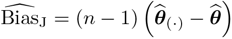
If $\hat{θ}$ is a biased estimator of a population parameter θ, in the sense that $E (\hat{θ}) \neq θ$ , the jackknife estimate of its (mean) bias is defined as

{\hat{Bias}}_{J} = (n - 1) ({\hat{θ}}_{(\cdot)} - \hat{θ})

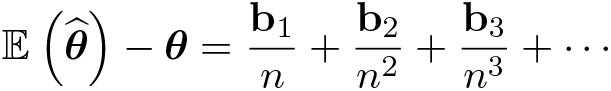
Suppose that $\hat{θ}$ has a finite bias of order 1/n; that is,

E (\hat{θ}) - θ = \frac{b_{1}}{n} + \frac{b_{2}}{n^{2}} + \frac{b_{3}}{n^{3}} + \dots

with b ₁ ≠ 0. Then, the bias of the jackknife bias-corrected estimator $\tilde{θ} = \hat{θ} - {\hat{Bias}}_{J}$ is

E (\tilde{θ}) - θ = - \frac{b_{2}}{n (n - 1)} - \frac{(2 n - 1) b_{3}}{n^{2} {(n - 1)}^{2}} + \dots

which is of the smaller order 1/n ². This argument relies on the existence of first moments, so it works only for overidentified 2sls and fe-2sls estimators with r ≥ k + 1. Jackknife bias-corrected 2SLS estimators were first proposed by Owen and Phillips (1975). Related estimators have been proposed by Angrist, Imbens, and Krueger (1999), Blomquist and Dahlberg (1999), Hahn, Hausman, and Kuersteiner (2004), and Ackerberg and Devereux (2009). The actual performance of these estimators in finite samples typically depends on the strength of the instruments.

4 Model selection

Model selection is about choosing, from a given set of models, one that is best in terms of out-of-sample prediction. It differs from hypothesis testing, which is instead about deciding whether the available data support a particular model against some alternatives. The distinguishing features of model selection are the emphasis on predictive accuracy and the concern for overfitting.

A variety of model-selection criteria are available, including the adjusted R ², Mallow’s C_p (Mallows 1973), and information criteria such as the Akaike information criterion (Akaike 1973) and the Bayesian information criterion (Schwarz 1978). All of these criteria may be regarded as analytical approximations to measures of out-of-sample predictive risk.

An alternative approach, purely data driven, is CV. Its simplest version is sample splitting, which randomly divides the data in two halves, one used to fit a model (the “training set”) and the other to assess predictive accuracy (the “validation set”). The mean squared error for the validation set provides an estimate of the mean squared prediction error (MSPE). Though easy to implement, sample splitting uses the data asymmetrically and inefficiently and tends to produce results that are highly variable.

An alternative method, K-fold CV, randomly divides the data into K ≤ n groups or folds of about equal size n/K. Then, it iteratively holds out one of the folds, fitting the data in the other K − 1 folds and using the results to predict the outcomes in the held-out fold. Finally, it estimates the MSPE by averaging the prediction error over the K folds.

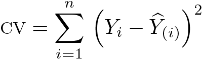
When K = n, this method is equivalent to holding out one observation at a time and then using the results to predict the held-out case. Because of this, n-fold CV is also known as leave-one-out cross-validation (L1OCV). The L1OCV criterion is defined as

CV = {\sum_{i = 1}^{n} (Y_{i} - {\hat{Y}}_{(i)})}^{2}

where ${\hat{Y}}_{(i)}$ is a predictor of Y_i that does not make use of Y_i . The l1ocv procedure

selects the model with the smallest cv.

The l1ocv criterion may be used to choose an appropriate value for “tuning param-

eters” such as the number of regressors in a linear model fit by ols or the number of instruments in an IV procedure. As argued by Varian (2014), “even if there is no tuning parameter, it is prudent to use cv to report goodness-of-fit measures because it measures out-of-sample performance, which is generally more meaningful than in-sample performance.”

4.1 OLS and IV

Because ${\hat{Y}}_{(i)} = X_{i}^{⊤} {\hat{β}}_{(i)}$ for a linear model fit by ols, the l1ocv criterion becomes

CV = \sum_{i = 1}^{n} {(\frac{{\hat{U}}_{i}}{1 - h_{i}})}^{2}

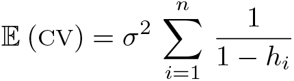
Under the classical homoskedastic linear model $E ({\hat{U}}_{i}^{2}) = (1 - h_{i}) σ^{2}$ , where σ ² is the variance of a regression error,

E (CV) = σ^{2} \sum_{i = 1}^{n} \frac{1}{1 - h_{i}}

If n is large enough and there are no high-leverage points, a first-order Taylor series expansion of (1 − h_i )⁻ ¹ about h_i = 0 gives

E (CV) \approx σ^{2} \sum_{i = 1}^{n} (1 + h_{i}) = (n + k) σ^{2}

Thus, in this case, cv is an approximately unbiased estimator of the mspe.

Similar criteria are easily constructed for simple iv, 2sls, fe, fe-iv, or fe-2sls estimates using (2)–(6).

5 Diagnostic checking

We focus on predictive residuals and measures of influence and leverage.

5.1 Predictive residuals

Predictive OLS residuals are defined as

{\hat{U}}_{(i)} = Y_{i} - X_{i}^{⊤} {\hat{β}}_{(i)} = \frac{{\hat{U}}_{i}}{1 - h_{i}} i = 1, \dots, n

The main advantage of predictive residuals is that they tend to give more emphasis to high-leverage points, because ${\hat{U}}_{(i)} \geq {\hat{U}}_{i}$ because 0 ≤ h_i ≤ 1. Notice that predictive residuals are in fact ubiquitous, because they are a part of (1), the formula for the jackknife estimate of the sampling variance of OLS, and the L1OCV criterion for OLS. Also notice that the predictive residuals are related to the internally Studentized residuals ${\hat{U}}_{i}^{S} = {\hat{U}}_{i} / \sqrt{s^{2} (1 - h_{i})}$ , with $s^{2} = {(n - k)}^{- 1} \sum_{i = 1}^{n} {\hat{U}}_{i}^{2}$ , which have approximately unit variance under the assumptions of the classical linear model. The externally Studentized residuals instead replace s ² by $s_{(i)}^{2} = {(n - k - 1)}^{- 1} \sum_{j \neq 1} {\hat{U}}_{(i)}^{2}$ .

Although Studentized residuals are defined only for ols, predictive residuals are easily defined for all other estimators we consider. For iv and 2sls, they are defined as

{\tilde{U}}_{(i)} = Y_{i} - X_{i}^{⊤} {\tilde{β}}_{(i)} i = 1, . . ., n

For fe, they are defined as

{\hat{U}}_{(i)}^{*} = Y_{i}^{*} - X_{i}^{*} {\hat{β}}_{(i)}^{*} i = 1, . . ., n

while for fe-iv and fe-2sls, they are defined as

{\tilde{U}}_{(i)}^{*} = Y_{i}^{*} - X_{i}^{*} {\hat{β}}_{(i)}^{*} i = 1, . . ., n

5.2 Measures of influence and leverage

To measure the overall influence of the ith observation on the ols estimates, Cook (1977) proposed the index

D_{i} = \frac{\sum_{j = 1}^{n} {(X_{j}^{⊤} {\hat{β}}_{(i)} - X_{j}^{⊤} \hat{β})}^{2}}{k s^{2}} = \frac{h_{i}}{1 - h_{i}} \frac{{({\tilde{U}}_{i}^{S})}^{2}}{k} i = 1, \dots, n

where ${\tilde{U}}_{i}^{S}$ is the ith internally Studentized residual. The index D_i is proportional to the norm of the eif of ols in the metric of the matrix X ^⊤ X. A large value of D_i indicates that the ith observation has a strong influence on the ols estimate. Cook and Weisberg (1982) suggest choosing D_i = 1 as a cutoff. An extension of Cook’s D-statistic to linear panel-data models was proposed by Banerjee and Frees (1997).

Notice that Cook’s distance may be written as $D_{i} = {(\hat{β} - {\hat{β}}_{(i)})}^{⊤} {\hat{V}}_{OLS}^{- 1} (\hat{β} - {\hat{β}}_{(i)}) / k$ , where ${\hat{V}}_{O L S} = s^{2} {(X^{⊤} X)}^{- 1}$ is the classical estimate of the sampling variance of ols, which assumes homoskedasticity. To avoid this assumption, we propose the following generalization,

D_{i}^{J} = \frac{1}{k} {(\hat{θ} - {\hat{θ}}_{(i)})}^{⊤} {\hat{V}}_{J}^{- 1} (\hat{θ} - {\hat{θ}}_{(i)}) i = 1, \dots, n

where $\hat{θ}$ is any of our linear estimators and ${\hat{V}}_{J}$ is the jackknife estimate of their sampling variance.

5.3 Diagnostic plots

A leverage plot shows on the x axis the leverage measure h_i /(1 − h_i ) and on the y axis the square of the internally Studentized residuals ${\tilde{U}}_{i}^{2}$ . These plots are very useful to detect the presence of outliers in the data and understand their nature but are not routinely produced by Stata.

6 The jackknife2 prefix command

jackknife2 is a prefix command written using Mata. The basic jackknife2 syntax, similar to the official jackknife prefix command, is as follows,

jackknife2 [, eif(filename[, replace]) hat(newvar[, replace])

fehat(filename[, replace]) presidual(newvar[, replace])

irstudent(newvar[, replace]) erstudent(newvar[, replace])

cooksd(newvar[, replace]) bpd(newvar[, replace]) dots(#) nodots]:

command

where command can be regress, xtreg with the fe option, ivregress2sls, or xtivreg with the fe option. Only pweight and iweight are allowed, even if command supports other weight types.

jackknife2 automatically computes the L1OCV criterion and the bias-corrected estimate. The latter, computed using the formula reported in section 3.2, is reported and stored in e(), while post diagnostics and measures of leverage are computed only when explicitly requested by the user through the corresponding options.

6.1 Options

eif( filename[, replace]) saves an Excel file (.xls) containing $n (\hat{θ} - {\hat{θ}}_{(i)})$ , the eif of the estimator. replace specifies that it is okay to replace filename if it already exists.

hat( newvar[, replace]) generates a new variable containing the diagonal elements of the relevant projection (“hat”) matrix. This option is available only when command is specified as regress or ivregress 2sls. replace specifies that it is okay to replace newvar if it already exists.

fehat( filename[, replace]) saves an Excel file (.xls) containing as many sheets as the number of diagonal blocks of the relevant projection (“hat”) matrix. replace specifies that it is okay to replace filename if it already exists. This option is available only when command is specified as xtreg, fe or xtivreg, fe. Notice that this option can be very time consuming when the number of clusters is large.

presidual( newvar[, replace]) generates a new variable containing the predictive residuals. replace specifies that it is okay to replace newvar if it already exists.

irstudent( newvar[, replace]) generates a new variable containing the internally Studentized residuals. This option is available only when command is specified as regress. replace specifies that it is okay to replace newvar if it already exists.

erstudent( newvar[, replace]) generates a new variable containing the externally Studentized residuals. This option is available only when command is specified as regress. replace specifies that it is okay to replace newvar if it already exists.

cooksd( newvar[, replace]) generates a new variable containing the value of Cook’s D-statistic (Cook 1977) and its extension to IV, 2SLS, or FE estimators. This option is available only when command is specified as regress, ivregress 2sls, or xtreg, fe. replace specifies that it is okay to replace newvar if it already exists.

bpd( newvar[, replace]) generates a new variable containing the generalization (9) of Cook’s D-statistic. replace specifies that it is okay to replace newvar if it already exists.

dots( # ) displays dots every # replications. dots(0) is a synonym for nodots.

nodots suppresses replication dots.

6.2 Implementation

Both jackknife and jackknife2 are built around a loop consisting of n iterations, one for each sample unit (cluster), but differ in the way the l1o estimate ${\hat{θ}}_{(i)}$ is computed at each iteration.

jackknife computes ${\hat{θ}}_{(i)}$ at each iteration by running the appropriate estimation command, for example, regress, on the subsample with the ith unit (cluster) removed. After exiting the loop, it then computes the jackknife estimate of variance using (7). This is computationally expensive because it involves solving the k ols normal equations n times.

jackknife2 instead computes ${\hat{θ}}_{(i)}$ at each iteration using the l1o formula, for example, (1) for OLS. Within the loop, it also accumulates the ingredients for the final computation of the jackknife estimates of variance and bias, the l1ocv criterion discussed in section 4, and the options listed in section 3.2. This substantially reduces the computational burden because the only heavy computation, for example, the inversion of X ^⊤ X for ols, is performed just once and outside the loop. Further, only the diagonal elements of certain high-dimensional matrices are needed, not the full matrices. For example, in the case of OLS, only the diagonal elements $h_{i} = X_{i}^{⊤} {(X^{⊤} X)}^{- 1} X_{i}$ of the n × n matrix H = X(X ^⊤ X)⁻ ¹ X ^⊤ are needed, not the full matrix. To reduce the computational burden, jackknife2 also exploits (2) when r = k and (3) when r > k.

7 Examples

7.1 Computing time: jackknife2 versus jackknife

In this section, we provide a comparison of the effective computing time needed for estimating jackknife standard errors using jackknife2 and jackknife.

We consider the following data-generating process,

\begin{array}{l} Y_{i t} = α_{i} + X_{i t}^{⊤} β + ϵ_{1 i t} \\ {\begin{array}{l} X_{1 i t}, \dots, X_{k i t} i.i.d. N (0, 1), & if ρ = 0 \\ \begin{array}{l} X_{1 i t} = δ_{i} + W_{1 i t} γ_{1} + W_{2 i t} γ_{2} + ϵ_{2 i t}, and \\ X_{2 i t}, \dots X_{k i t}, W_{1 i t}, W_{2 i t} i.i.d. N (0, 1), \end{array} & if ρ \neq 0 \end{array} \\ (\begin{array}{l} ϵ_{1 i t} \\ ϵ_{2 i t} \end{array}) ~ N_{2} ((\begin{array}{l} 0 \\ 0 \end{array}), [\begin{array}{l} 1 & ρ \\ ρ & 1 \end{array}]) \end{array}

with i = 1,…, n and t = 1,…, T .

This data-generating process encompasses all the cases covered by jackknife2, namely,

regress: OLS estimator for cross-sectional data (T = 1) with n = 10000 or 1000000, k = 10 or 100 exogenous regressors, α ₁ = · · · = α_n = 1, and ρ = 0;²

ivregress 2sls: 2SLS estimator for cross-sectional data (T = 1) with n = 10000 or 1000000, one endogenous regressor, k − 1 exogenous regressors (k = 10), two valid instruments, α ₁ = · · · = α_n = 1, δ ₁ = · · · = δ_n = 1, and ρ ≠ 0;

xtreg, fe: fe estimator for panel data with T = 2 or 10, n = 10000 or 1000000, k = 10 or 100 exogenous regressors, α ₁ ,…, α_n i.i.d. N(0, 1), and ρ = 0;

xtivreg, fe: fe-2sls estimator for panel data with T = 2 or 10, n = 10000 or 1000000, one endogenous regressor, k − 1 exogenous regressors (k = 10), two valid instruments, α ₁ ,…, α_n and δ ₁ ,…, δ_n i.i.d. N(0, 1), and ρ ≠ 0.

When ρ = 0, β ₁ ,…, β_k are all drawn independently from an N(0, 1) distribution. When ρ ≠ 0, β ₁ = 1, β ₂ ,…, β_k are drawn independently from an N(0, 1) distribution, and γ ₁ = γ ₂ = 0.5. We consider 18 exercises (4 for regress and xtivreg, fe, 2 for ivregress 2sls, and 8 for xtreg, fe), each containing two sets of estimates, one for jackknife and one for jackknife2. We run all of them using Stata/MP8 15.1 on a x64 desktop with an Intel i7-7820X 8 Cores 3.60 GHz processor with 32 gb of ram.

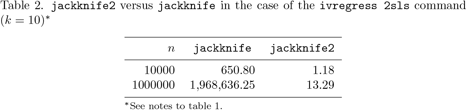
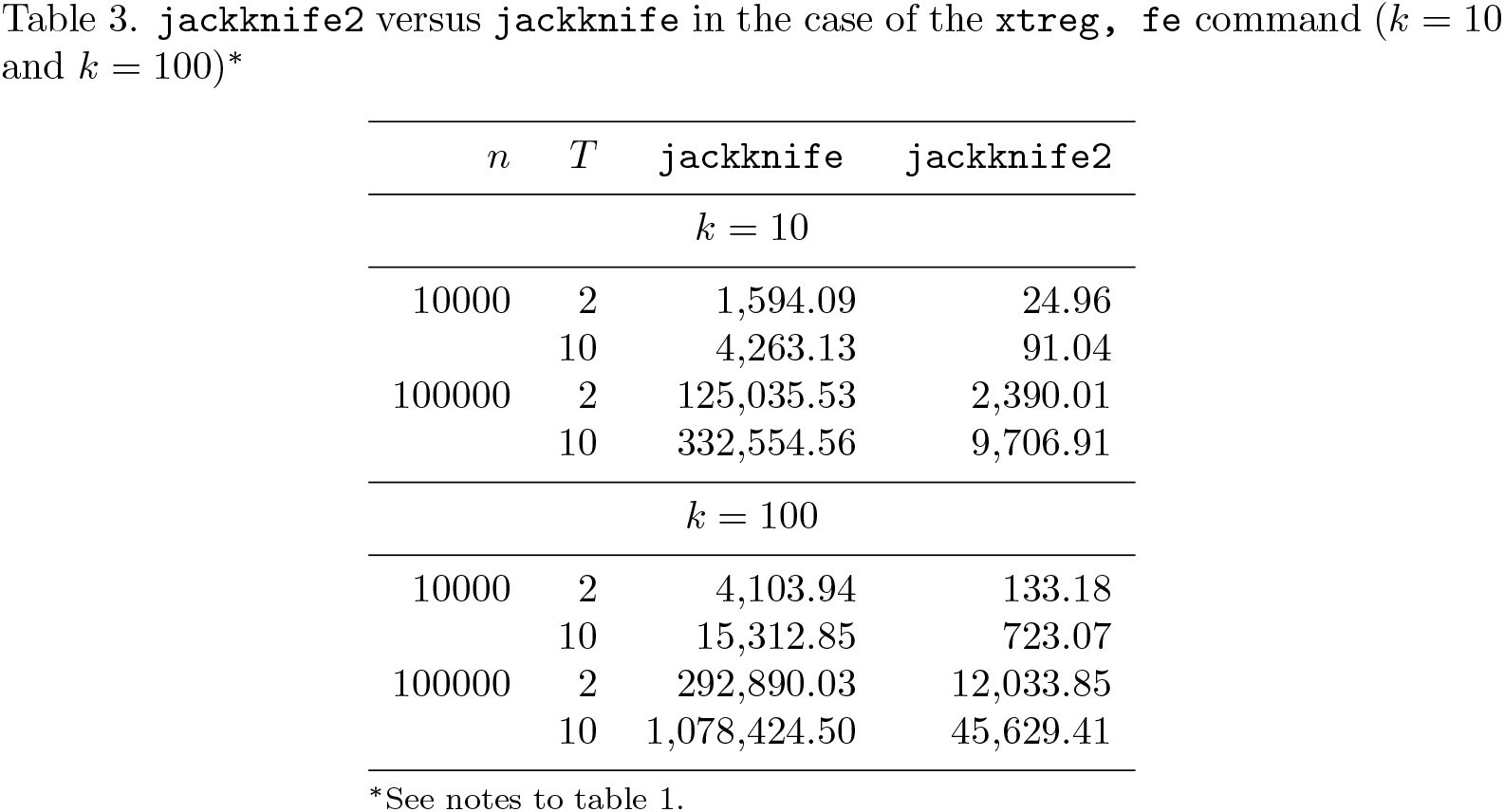
Results are reported in tables 1–4. The tables largely speak for themselves, showing substantial gains in computing time using jackknife2. When jackknife2 is used as a prefix for the regress command, the estimation is up to 18,121 times faster compared with jackknife (this occurs when n = 1000000 and k = 10). A huge gain is obtained also for the case of the ivregress 2sls command, where the estimation is up to 148,162 times faster (n = 1000000 and k = 10). Similarly, the estimation is up to 507 times faster in the case of xtivreg, fe (n = 10000 T = 2 and k = 10), while smaller gains (around, on average, 37 times faster) are obtained when jackknife2 is used with the xtreg, fe command.

Table 1.

jackknife2 versus jackknife in the case of the regress command (k = 10 and k = 100)^∗

n	k	jackknife	jackknife2
10000	10	105.70	0.11
	100	577.85	1.52
1000000	10	127,101.31	7.01
	100	1,104,862.50	604.51

∗Results are reported in seconds. Desktop x64 with Stata/MP8 15, Intel i7-7820X 8 Cores 3.60 GHz, 32 GB of RAM.

Table 2.

jackknife2 versus jackknife in the case of the ivregress 2sls command (k = 10)^∗

n	jackknife	jackknife2
10000	650.80	1.18
1000000	1,968,636.25	13.29

∗See notes to table 1.

Table 3.

jackknife2 versus jackknife in the case of the xtreg, fe command (k = 10 and k = 100)^∗

n	T	jackknife	jackknife2
k = 10
10000	2	1,594.09	24.96
	10	4,263.13	91.04
100000	2	125,035.53	2,390.01
	10	332,554.56	9,706.91
k = 100
10000	2	4,103.94	133.18
	10	15,312.85	723.07
100000	2	292,890.03	12,033.85
	10	1,078,424.50	45,629.41

∗See notes to table 1.

Table 4.

jackknife2 versus jackknife in the case of the xtivreg, fe command (k = 10)^∗

n	T	jackknife	jackknife2
10000	2	14,038.09	27.67
	10	52,015.40	108.26
100000	2	865,672.19	3,069.46
	10	3,096,145.75	18,277.38

∗See notes to table 1.

7.2 Leave-one-panel-out: jackknife2 versus cluster

In this section, we carry out a small Monte Carlo study comparing the performance of the jackknife in estimating the sampling variance of the FE estimator (see section 3.1) with that of its direct competitor, the clustered estimator (Stock and Watson 2008), implemented in Stata with the option vce(cluster). To our knowledge, this is the first time such a comparison has been made.

We consider the simple Gaussian linear panel-data model

Y_{i t} = α_{i} + X_{i t} β + ϵ_{i t}

where the logarithm of X_it is distributed as normal with mean α_i and unit variance. Notice that the lognormal distribution for X_it tends to generate isolated high-leverage points. As for the simulation of the unit-specific effects, we consider two cases: i) α_i distributed as standard normal; and ii) α_i distributed as the normal mixture 0.95 × N(0, 1) + 0.05 × N(5, 0.25).

Finally, we compare the cases of homoskedastic and heteroskedastic errors. In the first case, the ϵ_it ’s are generated as i.i.d. N(0, 1) pseudo–random variables, while in the second case, they are generated as independent $N (0, σ_{i t}^{2})$ pseudo–random variables with means zero and variance $σ_{i t}^{2} = 0.1 + 0.2 X_{i t} + 0.3 X_{i t}^{2}$ . Note that the latter ensures substantial heteroskedasticity, especially when the α_i ’s are generated according to the aforementioned mixture model.

We investigate the effect of varying the cross-sectional dimension (n = 1000 or 10000) or the panel length (T = 2 or 10). Each experiment involves M = 2000 replications, and there are 16 experiments in total (one for each combination of n and T, separately for homoskedastic and heteroskedastic errors and the two different models for the unit-specific effects α_i ).

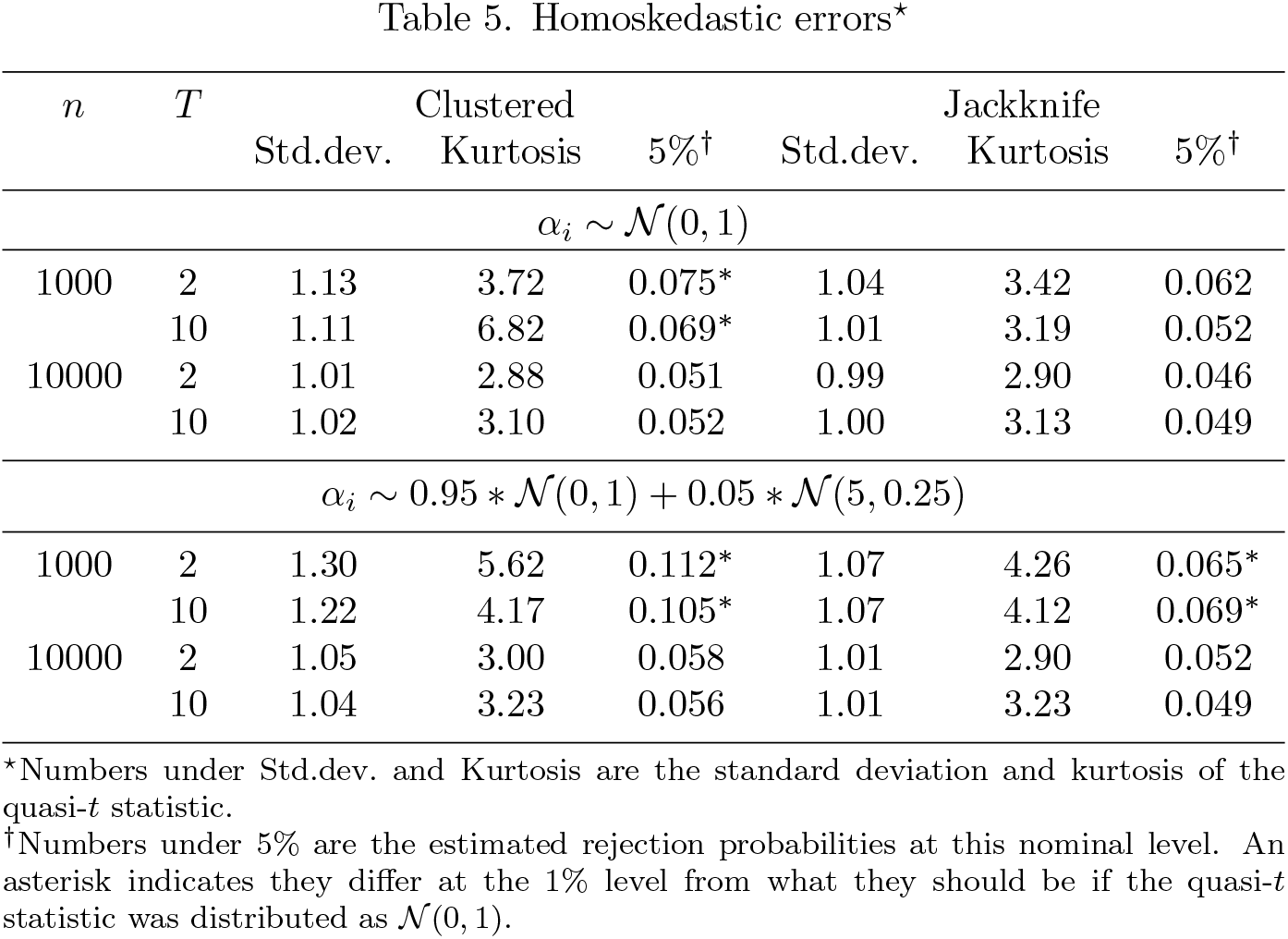
For each replication, we compute two “quasi-t” statistics for testing the hypothesis that β is equal to 1. These statistics, denoted by “Clustered” and “Jackknife”, exploit the covariance matrices after which they are named. For each experiment, we calculated the sample mean, standard deviation, skewness, and kurtosis (over the 2,000 replications) for both test statistics, but because there was nothing in the simulation results suggesting that they had a nonzero mean, or that their distributions were not symmetric, we report only the standard deviation (“Std.dev.”) and the kurtosis.³ To investigate how often we will be led to make invalid inferences by using the considered test statistics, we report rejection frequencies (“5%”) of the form $\hat{q} = R / M$ , where R is the observed number of rejections, that is, the number of times the test statistic exceeds the 1.96 critical value, and M is the number of replications.

Simulation results for all experiments are reported in tables 5 and 6. As in MacK-innon and White (1985), we find that almost all the test statistics have standard deviations greater than one, so that rejection frequencies based on them almost always exceed their 5% nominal size. As expected, these standard deviations tend to one as n or T increases. Interestingly, the distribution of the test statistics is close to standard normal when the errors are homoskedastic (table 5). Overall, the standard deviation and the kurtosis of the test statistic based on the clustered variance estimator exceed those of the statistic based on the jackknife variance. The difference between the two test statistics is striking, especially in the presence of heteroskedasticity and when the unit-specific effects are distributed as a normal mixture. Table 5 clearly shows that, even with moderate sample sizes (n = 1000 regardless of the panel length) and homoskedasticity, using the clustered variance estimator could easily lead to serious errors of inference. With n = 1000 and substantial heteroskedasticity, the jackknife also does not perform well. Its worst performance is when n = 1000, T = 2, and the distribution of the unit-specific effects is characterized by heteroskedasticity and outliers. In this case, the jackknife-based test incorrectly rejects the null hypothesis 9.7% of the time at the nominal 5% level. Still, it performs much better than its competitor because the clustered-based test rejects the null 22.2% of the time.

Table 5.

Homoskedastic errors ^⋆

n	T		Clustered		Jackknife
		Std.dev.	Kurtosis	5%^†	Std.dev.	Kurtosis	5%^†
α_i ∼ N(0, 1)
1000	2	1.13	3.72	0.075^∗	1.04	3.42	0.062
	10	1.11	6.82	0.069^∗	1.01	3.19	0.052
10000	2	1.01	2.88	0.051	0.99	2.90	0.046
	10	1.02	3.10	0.052	1.00	3.13	0.049
α_i ∼ 0.95 ∗ N(0, 1) + 0.05 ∗ N(5, 0.25)
1000	2	1.30	5.62	0.112^∗	1.07	4.26	0.065^∗
	10	1.22	4.17	0.105^∗	1.07	4.12	0.069^∗
10000	2	1.05	3.00	0.058	1.01	2.90	0.052
	10	1.04	3.23	0.056	1.01	3.23	0.049

⋆Numbers under Std.dev. and Kurtosis are the standard deviation and kurtosis of the

quasi-t statistic.

†Numbers under 5% are the estimated rejection probabilities at this nominal level. An

asterisk indicates they differ at the 1% level from what they should be if the quasi-t statistic was distributed as N(0, 1).

Table 6.

Heteroskedastic errors ^⋆

n	T		Clustered			Jackknife
		Std.dev.	Kurtosis	5%	Std.dev.	Kurtosis	5%
α_i ∼ N(0, 1)
1000	2	1.49	7.78	0.141^∗	1.15	3.69	0.064^∗
	10	1.36	4.09	0.132^∗	1.11	3.03	0.068^∗
10000	2	1.16	3.85	0.075^∗	1.06	2.90	0.056
	10	1.14	2.76	0.078^∗	1.06	2.68	0.056
α_i ∼ 0.95 ∗ N(0, 1) + 0.05 ∗ N(5, 0.25)
1000	2	2.66	82.68	0.222^∗	1.34	11.61	0.097^∗
	10	1.59	5.68	0.179^∗	1.21	4.21	0.093^∗
10000	2	1.21	3.29	0.094^∗	1.07	2.96	0.062
	10	1.14	3.17	0.084^∗	1.04	3.02	0.057

⋆See notes to table 5.

8 Conclusions

Although the jackknife is potentially very useful, its current implementation in Stata is very general and also inefficient for linear estimators. In this article, we described the new prefix command jackknife2, which computes jackknife standard errors and other useful statistics, such as CV criteria, predictive residuals, and measures of influence and leverage, much faster than the official jackknife command. The new prefix command can be used when the model is fit via the regress, ivregress 2sls, xtreg, fe, and xtivreg, fe official Stata commands. We reported a comparison of the effective computing time needed for the estimation of the jackknife standard errors using jackknife and jackknife2, documenting the huge benefits in terms of computing time obtainable using the new prefix command. We also reported Monte Carlo evidence comparing the performance of the jackknife and its direct competitor, the clustered estimator, in estimating the sampling variance of the FE estimator.

Supplemental Material

Supplemental Material, st0617 - Fast leave-one-out methods for inference, model selection, and diagnostic checking

Supplemental Material, st0617 for Fast leave-one-out methods for inference, model selection, and diagnostic checking by Federico Belotti and Franco Peracchi in The Stata Journal

Footnotes

9 Acknowledgments

We thank Roberto Rocci and Alwyn Young for useful discussions and an anonymous referee for very detailed comments. Franco Peracchi acknowledges financial support from MIUR PRIN 2015FMRE5X.

10 Programs and supplemental materials

To install a snapshot of the corresponding software files as they existed at the time of publication of this article, type

Notes

References

Ackerberg

D. A.

Devereux

P. J.

. 2009. Improved JIVE estimators for overidentified linear models with and without heteroskedasticity. Review of Economics and Statistics 91: 351–362. https://doi.org/10.1162/rest.91.2.351.

Akaike

1973. Information theory and an extension of the maximum likelihood principle. In Second International Symposium on Information Theory, ed. Petrov

B. N.

Cs´aki

, 267–281. Budapest, Hungary: Akademiai Kiado.

Angrist

J. D.

Imbens

G. W.

Krueger

A. B.

. 1999. Jackknife instrumental variables estimation. Journal of Applied Econometrics 14: 57–67. https://doi.org/10.1002/(SICI)1099-1255(199901/02)14:1 h 57::AID-JAE501 i 3.0.CO;2-G.

Banerjee

Frees

E. W.

. 1997. Influence diagnostics for linear longitudinal models. Journal of the American Statistical Association 92: 999–1005. https://doi.org/10.2307/2965564.

Blomquist

Dahlberg

. 1999. Small sample properties of LIML and jackknife IV estimators: Experiments with weak instruments. Journal of Applied Econometrics 14: 69–88. https://doi.org/10.1002/(SICI)1099-1255(199901/02)14:1 h 69::AID-JAE521 i 3.0.CO;2-7.

Cameron

A. C.

Miller

D. L.

. 2015. A practitioner’s guide to cluster–robust inference. Journal of Human Resources 50: 317–372. https://doi.org/10.3368/jhr.50.2.317.

Chesher

1989. H´ajek inequalities, measures of leverage and the size of heteroskedasticity robust Wald tests. Econometrica 57: 971–977. https://doi.org/10.2307/1913779.

Chesher

Jewitt

. 1987. The bias of a heteroskedasticity consistent covariance matrix estimator. Econometrica 55: 1217–1222. https://doi.org/10.2307/1911269.

Cook

R. D.

1977. Detection of influential observation in linear regression. Technometrics 19: 15–18. https://doi.org/10.2307/1268249.

10.

Cook

R. D.

Weisberg

. 1982. Residuals and Influence in Regression. New York: Chapman & Hall.

11.

Davidson

MacKinnon

J. G.

. 2007. Moments of IV and JIVE estimators. Econometrics Journal 10: 541–553. https://doi.org/10.1111/j.1368-423X.2007.00221.x.

12.

Efron

1982. The Jackknife, the Bootstrap and Other Resampling Plans. Philadelphia: Society for Industrial and Applied Mathematics.

13.

Hahn

Hausman

Kuersteiner

. 2004. Estimation with weak instruments: Accuracy of higher-order bias and MSE approximations. Econometrics Journal 7: 272–306. https://doi.org/10.1111/j.1368-423X.2004.00131.x.

14.

Hinkley

D. V.

1977. Jackknifing in unbalanced situations. Technometrics 19: 285–292. https://doi.org/10.2307/1267698.

15.

Horn

S. D.

Horn

R. A.

Duncan

D. B.

. 1975. Estimating heteroscedastic variances in linear models. Journal of the American Statistical Association 70: 380–385. https://doi.org/10.2307/2285827.

16.

MacKinnon

J. G.

White

. 1985. Some heteroskedasticity-consistent covariance matrix estimators with improved finite sample properties. Journal of Econometrics 29: 305–325. https://doi.org/10.1016/0304-4076(85)90158-7.

17.

Mallows

C. L.

1973. Some comments on C_p . Technometrics 15: 661–675. https://doi.org/10.2307/1267380.

18.

Miller

R. G.

1974. The jackknife—A review. Biometrika 61: 1–15. https://doi.org/10.1093/biomet/61.1.1.

19.

Owen

A. D.

Phillips

G. D. A.

. 1975. Bias reduction and approximate confidence intervals for the jackknifed 2SLS estimator. Paper presented to the World Congress of the Econometric Society, Toronto.

20.

Peracchi

2001. Econometrics. Chichester, UK: Wiley.

21.

Phillips

G. D. A

. 1977. Recursions for the two-stage least-squares estimators. Journal of Econometrics 6: 65–77. https://doi.org/10.1016/0304-4076(77)90055-0.

22.

Quenouille

M. H.

1956. Notes on bias in estimation. Biometrika 43: 353–360. https://doi.org/10.1093/biomet/43.3-4.353.

23.

Schwarz

1978. Estimating the dimension of a model. Annals of Statistics 6: 461–464. https://doi.org/10.1214/aos/1176344136.

24.

Shao

C. F. J.

. 1989. A general theory for jackknife variance estimation. Annals of Statistics 17: 1176–1197. https://doi.org/10.1214/aos/1176347263.

25.

Stock

J. H.

Watson

M. W.

. 2008. Heteroskedasticity-robust standard errors for fixed effects panel data regression. Econometrica 76: 155–174. https://doi.org/10.1111/j.0012-9682.2008.00821.x.

26.

Stone

1974. Cross-validatory choice and assessment of statistical predictions. Journal of the Royal Statistical Society, Series B 36: 111–133. https://doi.org/10.1111/j.2517-6161.1974.tb00994.x.

27.

Stone

1977. Asymptotics for and against cross-validation. Biometrika 64: 29–35. https://doi.org/10.1093/biomet/64.1.29.

28.

Tukey

J. W.

1958. Bias and confidence in not-quite large samples. Annals of Mathematical Statistics 29: 614. https://doi.org/10.1214/aoms/1177706647.

29.

Varian

H. R.

2014. Big data: New tricks for econometrics. Journal of Economic Perspectives 28: 3–28. https://doi.org/10.1257/jep.28.2.3.

30.

Young

2020. Consistency without inference: Instrumental variables in practical application. http://personal.lse.ac.uk/YoungA/CWOI.pdf.

Supplementary Material

Please find the following supplemental material available below.

For Open Access articles published under a Creative Commons License, all supplemental material carries the same license as the article it is associated with.

For non-Open Access articles published, all supplemental material carries a non-exclusive license, and permission requests for re-use of supplemental material or any part of supplemental material shall be sent directly to the copyright owner as specified in the copyright notice associated with the article.

0.00 MB

Fast leave-one-out methods for inference,model selection,and diagnostic checking

Abstract

Keywords

1 Introduction

2 The basic L1O formula

2.1 Cross-sectional data

OLS estimation

IV estimation

2.2 Panel data

Fixed-effects estimation

Fixed-effects IV estimation

3 Inference

3.1 Estimating sampling variability

3.2 Correcting for bias

4 Model selection

4.1 OLS and IV

5 Diagnostic checking

5.1 Predictive residuals

5.2 Measures of influence and leverage

5.3 Diagnostic plots

6 The jackknife2 prefix command

6.1 Options

6.2 Implementation

7 Examples

7.1 Computing time: jackknife2 versus jackknife

7.2 Leave-one-panel-out: jackknife2 versus cluster

8 Conclusions

Supplemental Material

Supplemental Material, st0617 - Fast leave-one-out methods for inference, model selection, and diagnostic checking

Footnotes

9 Acknowledgments

10 Programs and supplemental materials

Notes

References

Supplementary Material