
Abstract
Nonparametric regressions are powerful statistical tools that can be used to model relationships between dependent and independent variables with minimal assumptions on the underlying functional forms. Despite their potential benefits, these models have two weaknesses: The added flexibility creates a curse of dimensionality, and procedures available for model selection, like crossvalidation, have a high computational cost in samples with even moderate sizes. An alternative to fully nonparametric models is semiparametric models that combine the flexibility of nonparametric regressions with the structure of standard models. In this article, I describe the estimation of a particular type of semiparametric model known as the smooth varying-coefficient model (Hastie and Tibshirani, 1993, Journal of the Royal Statistical Society, Series B 55: 757–796), based on kernel regression methods, using a new set of commands within
Keywords
1 Introduction
Nonparametric regressions are powerful statistical tools that can be used to model relationships between dependent and independent variables with minimal assumptions on the underlying functional forms. This flexibility makes nonparametric regressions robust to functional form misspecification, which is one of the main advantages over standard regression analysis.
The added flexibility of nonparametric regressions comes at a cost. On the one hand, the added flexibility creates what is known as the curse of dimensionality. In essence, because nonparametric regressions imply the estimation of many parameters, accounting for interactions and nonlinearities, more data are required to obtain results with a similar level of precision to their parametric counterparts. On the other hand, while larger datasets can be used to reduce the curse of dimensionality, procedures used for model selection and estimations are often too computationally intensive, making the estimation of this type of model less practical in samples of moderate to large sizes. Perhaps because of these limitations, and until recent versions, Stata had a limited set of native commands for the estimation of nonparametric models. Even with the recent development of computing power, the estimation of full nonparametric models, using the currently available commands, remains a challenge when using large samples. 1
One response to the main weakness of nonparametric methods has been the development of semiparametric methods. These methods combine the flexibility of nonparametric regressions with the structure of standard parametric models, reducing the curse of dimensionality and the computational cost of model selection and estimation. 2 In fact, many community-contributed commands have been proposed for the analysis of a large class of semiparametric models in Stata. 3
A particular type of semiparametric model, the estimation of which has not been explored within Stata, is known as the smooth varying-coefficient model (SVCM) (Hastie and Tibshirani 1993). These models assume that the outcome Y is a function of two sets of characteristics,
For example, as described in Hainmueller, Mummolo, and Xu (2019), SVCMs can be thought of as multiplicative interactive models where the variable
In this article, I introduce a new set of commands that aims to facilitate the model selection, estimation, and visualization of SVCMs with a single smoothing variable
The rest of the article is structured as follows. Section 2 reviews the estimation of SVCMs. Section 3 provides a detailed review of the implementation procedures and commands used for model selection, estimation, and postestimation. Section 4 illustrates the commands, and section 5 concludes.
2 Nonparametric regression and SVCM
2.1 Nonparametric regressions
Consider a model where Y is the dependent variable and

Essentially, this model specification implies that

where

and Kj (Wij, wj, hwj ) is a kernel function defined by the point of reference wj and the bandwidth hwj : 4

This function K(·) gives more weight to observations that are close to the point
An alternative procedure is to estimate g(

As described in Li and Racine (2007) and Stinchcombe and Drukker (2013), in the case of kernel methods, the effective number of observations for the estimation of the conditional mean decreases rapidly as k increases and
2.2 SVCM
SVCMs, as introduced by Hastie and Tibshirani (1993), assume that there is some structure in the model. Instead of estimating a function like (1), the authors suggest distinguishing two types of independent variables,

This specification reduces the problem of the curse of dimensionality of the fit model compared with (1) by assuming
For example, Li et al. (2002) analyze the production function of the nonmetal mineral manufacturing industry in China by analyzing the marginal productivity of capital and labor (
Just like with nonparametric regressions, various methods have been proposed for the estimation of this type of model. Hastie and Tibshirani (1993) suggest estimating β(
2.3 SVCM: Local kernel estimator
Consider a simplified version of the SVCM [(4)], as described in Li et al. (2002), where Y is the dependent variable, Z is a single continuous variable, and
Following Li and Racine (2007), the coefficients in (4) can be derived as follows. Starting from (4), premultiply both sides by

Using sample data, (5) can be an unfeasible estimator of β(z) because there may be few or no observations for which Zi = z, making β(z) impossible to estimate. 7 As an alternative, a feasible estimation for (3) can be obtained using kernel methods for any point z,

or the equivalent in matrix form,

where k(·) is the kernel function, as defined in (2), that gives more weight to observations where Zi is closer to z, given the bandwidth h. K h (z) is an N ×N diagonal matrix with the ith element equal to k{(Zi − z)/hz }. Equation (6) constitutes the local constant (LC) estimator of SVCM.
A drawback of the LC estimator is that it is well known for its potentially large bias when estimating functions near boundaries of the support of Z. A simple solution to reduce this bias is to use a local linear (LL) estimator, based on a first-order approximation of the coefficients β(Zi ). This implies that instead of estimating (4), one can instead fit the following model:

This implies that an approximation for yi can be obtained using a linear expansion with respect to β(z) and that the closer Zi is to z, the more accurate the approximation will be.
Define X
i
= {

where
2.4 Example: SVCM and weighted least squares
While it may not seem evident, (4) and (7) show that the estimation of SVCMs using kernel methods can be easily obtained using weighted ordinary least squares (OLS), where weights are defined by the kernel functions. To show this, let’s consider the dataset “Fictional data on monthly drunk driving citations” (
Say that you are interested in analyzing how the effect of
In general, it may be more convenient to fit the model using kernel functions as weights. As discussed in the literature, the choice of kernel function is not as important as the choice of bandwidth. For simplicity, I will use a Gaussian kernel with a bandwidth h = 0.5. This is directly implemented using the
This example implements the LC estimators following (5). For the implementation of the LL estimator, an auxiliary variable needs to be constructed (Zi − z)
To show how these models compare with each other, figures 1a and 1b provide a simple plot of the coefficients associated with

Varying-coefficient models (VCM) across fines: college and taxes
“VCM-Exact” corresponds to the models that constrain data to Zi
= z, whereas “SVCM-LC” and “SVCM-LL” indicate the estimates come from the LC and LL estimators of the SVCM model, respectively. Note that there are no estimations for the “VCM- Exact” model at the boundaries of the distribution of
While this simple illustration shows the simplicity of fitting SVCMs, there are many details regarding model choice and statistical inference that require further examination. In the next section, I discuss some of the details regarding these problems, introducing the commands in
3 SVCM: vc_pack
3.1 Model selection: vc_bw and vc_bwalt
Leave-one-out CV
The most important aspect of the estimation of SVCMs is the choice of the bandwidth parameter h. While larger bandwidths may help to reduce the variance of the estimations by allowing more information to be used on the local estimation process, it will increase the bias of the estimators by restricting the model flexibility. In contrast, smaller bandwidths can reduce bias, allowing for greater flexibility in the estimation but at the cost of higher variability. 9
The illustration presented in the previous section is an example of this phenomenon. The standard OLS coefficients can be considered as an extreme scenario, where the bandwidth h is so large that all observations receive equal weight regardless of the point of interest. This is guaranteed to obtain the minimum variance for the estimated parameters but with a potentially large cost in terms of model bias. On the opposite side of the spectrum, the results where the regressions are estimated using samples restricted to observations with a specific value of
While there are many suggestions in the literature regarding bandwidth selection (see, for example, Zhang and Lee [2000]), the methodology used here is based on a leave-one-out CV procedure. Consider the model described in (4) and a sample of size N. The optimal bandwidth h∗ is such that it minimizes the CV criteria defined as

where
On the one hand, even if Z is a continuous variable in nature, it is often recorded as partially discrete data. A person’s age, for example, is a variable that is continuous in nature but is often measured in years. This implies that the number of distinct coefficients
On the other hand, the estimation of the CV(h) does not require the explicit estimation of

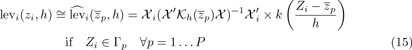
where lev
i
(zi, h) is the local leverage statistic, defined as the ith diagonal element of the local projection matrix

Using this shortcut, we can rewrite CV(h) to reflect only the number of necessary regressions that need to be estimated. Consider the vector

While (11) shows the number of estimated equations (J) is potentially smaller than the total number of observations in the sample (N), in some applications J may still be too large to allow for a fast estimation of CV(·). A feasible alternative in such cases is to use what Hoti and Holmström (2003) and Ichimura and Todd (2007) denominate as block or binned LL regressions to obtain an approximation of the CV criteria.
Consider the vector
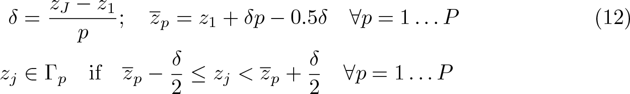
Instead of estimating J sets of parameters, for each distinct value of Z, one estimates P sets of parameters using the points of reference


Using these expressions, we can approximate the leave-one-out error (

This can be used to obtain an alternative expression for the CV criteria,

which reduces the number of estimated equations from J to P . We can see that as the number of groups P increases and the smaller the bin width δ is, the better the approximation of
Automatic model selection

stopping when ht and ht− 1 are sufficiently close and selecting h∗ = ht . The firstand second-order derivatives are estimated using numerical methods with three points of reference. The scalar A is equal to 1 as long as there is an improvement in the maximization process [that is, CV(ht ) < CV(ht− 1)]. Otherwise, A is reduced by half until an improvement is found.
Both commands use the following syntax:
depvar is the dependent variable Y , indepvars is the list of all independent variables
The default is to use all distinct values in the smoothing variable, up to 500 distinct values. When more than 500 distinct values are detected, the command uses the options
Using the option
After finishing the minimization process, the program stores the optimal bandwidth, the kernel function, and the smoothing variable name as globals:
3.2 Model estimation and inference: vc_reg, vc_preg, and vc_bsreg
Estimation of the variance–covariance matrix
As shown in section 2, once the bandwidth is selected, the estimation of the SVCM is a simple process that requires three steps:
Select the point or points of interest for which the model will be fit (typically a subset of all possible values of the smoothing variable z). Construct the appropriate kernel weights based on the points of interest, selected kernel function, and the optimal bandwidth h∗
. Construct the auxiliary variable (Zi − z), which will be interacted with all independent variables in the model.
Once the auxiliary variables have been created, one can obtain the model coefficients and their gradients, conditional on all the selected points of interest, by estimating (7) using kernel-weighted least squares as in (8). The next step is the estimation of standard errors of the estimated parameters to obtain statistical inferences from the SVCM.
Following Li et al. (2002) and Li and Racine (2007, 2010), a feasible estimator for the asymptotic variance–covariance matrix of the SVCM, given a point of interest z and bandwidth h∗ , can be obtained as follows: 14

Following the literature on the estimation of robust standard errors under heteroskedasticity (Long and Ervin 2000), one can estimate the variance–covariance matrix, substituting
There is a debate regarding the use of analytical variance–covariance matrices in the framework of nonparametric kernel regressions. Cattaneo and Jansson (2018) advocate for the use of resampling methods, specifically paired bootstrap samples, to correctly estimate the variance–covariance matrix of the estimated coefficients when fitting kernel-based semiparametric models. In fact, they indicate percentile-based confidence intervals provide better coverage because paired bootstrap automatically corrects for nonnegligible estimation bias.
15
Broadly speaking, the paired bootstrap procedure, adapted to the estimation of SVCMs, is as follows:
Using the original sample Obtain a paired bootstrap sample B with replacement from the original sample, and estimate Repeat 2 M times. The bootstrap standard errors for the coefficients are defined as

where
Implementation: vc_reg, vc_preg, and vc_bsreg
While
The three commands share the same basic syntax:
As with
Because the richness of SVCM comes from the estimation of the linear effects as a function of the smoothing variable Z, these commands offer two alternatives to select the points of interest over which the local regressions will be estimated. The option
Because
When estimating a single equation,
3.3 Model postestimation: vc_predict and vc_test
In addition to the options previously described,
Residuals and leverage from this command can be used, for example, for the estimation of SVCMs using
Log mean squared leave-one-out errors
Consider the SVCM described in (4). Given the smoothing variable Z (svar), kernel function (
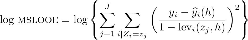
when no binning option is used, or its approximation,

when binning options (
Goodness-of-fit R 2

which is the same one used by

When binning options are used,
Model and residual degrees of freedom
The effective number of degrees of freedom is a statistic that has proven useful in the literature of nonparametric econometrics for the comparison of models with different types of smoothers. Following the terminology from Hastie and Tibshirani (1990), consider any parametric and nonparametric model with a projection matrix

In the context of linear regression models, where the projection matrix
For the specific case of SVCMs, the projection matrix

where γzj is an N × N matrix with the ith diagonal element equal to 1 if Zi = zj and 0 elsewhere. This implies that the first measure of degrees of freedom is equivalent to

The second measure of degrees of freedom is computationally more difficult to estimate because it requires N 2 operations. As an alternative, Hastie and Tibshirani (1990) suggest using the following approximation:

Expected kernel observations
One of the drawbacks of nonparametric regression analysis is the more rapid the decline of the effective number of observations used for the estimation of the parameters of interest, the larger the number of explanatory variables used in the model (the curse of dimensionality) and the smaller the bandwidths. To provide the user with a statistic summarizing the amount of information used through the estimation process, researchers commonly report n|h| as the expected number of kernel observations E(Kobs), where |h| is the product of all bandwidths of the explanatory variables. 16 This statistic, however, can be misleading.
Consider the estimation of a model with a single independent variable for which an optimal bandwidth h∗ is selected. If the scale of the independent variable doubles, the optimal bandwidth of the rescaled variable will double, but E(Kobs) should remain the same. The statistic n|h|, however, suggests that the E(Kobs) has doubled as well. 17
As an alternative measure to n|h|, I propose a statistic based on what I denominate standardized kernel weights Kw (Zi, z, h), which are defined as 18

These kernel weights are guaranteed to fall between 0 and 1. While this change in the scale of local weights has no impact on the estimation of the point estimates of the models, it provides a more intuitive understanding of the role of weights in the estimation process. Observations where Zi is equal to z will receive a weight of 1, and one can consider that the information of that observation is fully used when estimating the LL regression. If an observation has a kw (·) of, say, 0.5, one can consider that the information contributed by that observation to the local kernel regression is half of an observation where Zi = z. Finally, observations with a kw (·) = 0 do not contribute to the local estimation at all. These kernel weights can be used to estimate the effective number of observations {Kobs(z)} used for the estimation of the parameters of interest for a given point of reference z: 19

Because areas with higher density use more observations than areas where z is sparsely distributed, the expected number of kernel observations E(Kobs) can be defined as the simple weighted average of Kobs(zj ) using all observations in the sample. This leads to

where Nj is the number of observations with Zi = zj . When binning options are used, the estimator is

where Np is the number of observations that fall within the pth bin.
If Z is continuous, this statistic has two convenient properties with respect to the bandwidth h:

This provides a more intuitive understanding of the effect of the bandwidth on the average amount of information used for the estimation of local regressions compared with the standard parametric model. At least, there will be one observation for the estimation of the local estimation, and at most, all the data will be used for each local estimation. This statistic is also reported after
Specification tests
In addition to reporting the basic summary statistics described above,


q is the number of explanatory variables defined in

The null hypothesis (H
0) is that the parametric model 0, 1, 2, or 3 is correctly specified, whereas the alternative hypothesis is that the SVCM is correct. While the exact distribution of this statistic is not known, Hastie and Tibshirani (1990, 65) suggest using critical values for an F statistic with n − df2 degrees of freedom in the numerator and df2 − df
p
degrees of freedom in the denominator, a rough test for a quick inspection of the model specification. When binning options are used,
Cai, Fan, and Yao (2000) specification test: vc_test
Because the exact distribution of the approximate F statistic is not known,
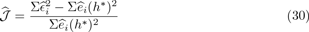
where
Because the distribution of the statistic J is not known, a wild bootstrap procedure can be used to obtain its empirical distribution using the following procedure:
Define Construct a new dependent variable
vi
follows a Bernoulli distribution with Using the new dependent variable Repeat 2 and 3 enough times to obtain the empirical distribution of the statistic J.

If
The command
As with previous commands, one has to specify the dependent and independent variables in the model, but specifying
3.4 Model visualization: vc_graph
One attractive feature of semiparametric models in general, and SVCMs in particular, is the potential to visualize effects across the range of the explanatory variables that enter the model nonparametrically. These plots can be used for a richer interpretation of marginal effects. As described in section 3.2, when
varlist can contain a subset of all independent variables used in the estimation of the SVCM. If factor variables and interactions are used, the same format must be used when using
rather than normal-based intervals. This option cannot be used with
4 Illustration: Determinants of drunk driving citations: The role of fines
For this illustration, I use the fictitious
I start the analysis by using

The command suggests a bandwidth of 0.7398, suggesting the bandwidth used in section 2.4 may have been undersmoothing the results.
Next, I obtain simple summary statistics of the model using

The report indicates that the model uses approximately 18.7 degrees of freedom [(22)], whereas the residuals have 477.15 degrees of freedom [(23)]. The model has an R
2
that is larger than the simple regression model (
The approximate F test suggests rejecting models 0 and 1 in favor of the SVCM, but one cannot reject the null hypothesis that a model with a quadratic interaction with fines is correctly specified. The local fit of the model with a cubic interaction seems to be better than the SVCM, which explains why the F statistic is negative. I also use

The results are consistent with the approximate F statistic. In the first case, the J statistic of the model is 0.16869, which is larger than the 97.5th percentile of the empirical distribution of the statistic, suggesting the rejection of the null of a linear interaction. The test comparing with the parametric quadratic interaction model is less conclusive. The J statistic is 0.0141, which suggests rejection of the null at 10% of confidence, but the null cannot be rejected at 5%. Despite these results, I will go ahead and fit the SVCM.
To provide an overview of the results that are similar to the output of standard regression models, I provide the conditional effects using the 10th, 50th, and 90th percentiles of fines as the points of reference, which correspond to 9, 10, and 11. This is done with the three commands available in

The results from these regressions are shown in table 1, columns 2–4, showing the standard errors obtained with all three commands (robust, F robust, and bootstrap). Column 1 presents the results for the standard regression model. For the SVCM, two subcolumns are provided. The left subcolumn shows the conditional effects β(z), whereas the right subcolumn shows the gradient of that effect ∂β(z)/∂z.
Determinants of number of monthly citations, conditional on fines. SVCM

NOTES: Robust std err corresponds to the output with
Overall, robust standard errors obtained with the LL approximation (
To complement the information in this table and before we provide an interpretation of the results, figure 2 provides a plot with 95% confidence intervals for the conditional effects of all variables in the model, using a predefined set of points of interest. I first use

The main difference with the previous examples is that the option

SVCM: Conditional effects across fines
If one is interested in the gradients ∂β(z)/∂z, they can be plotted using the following commands:
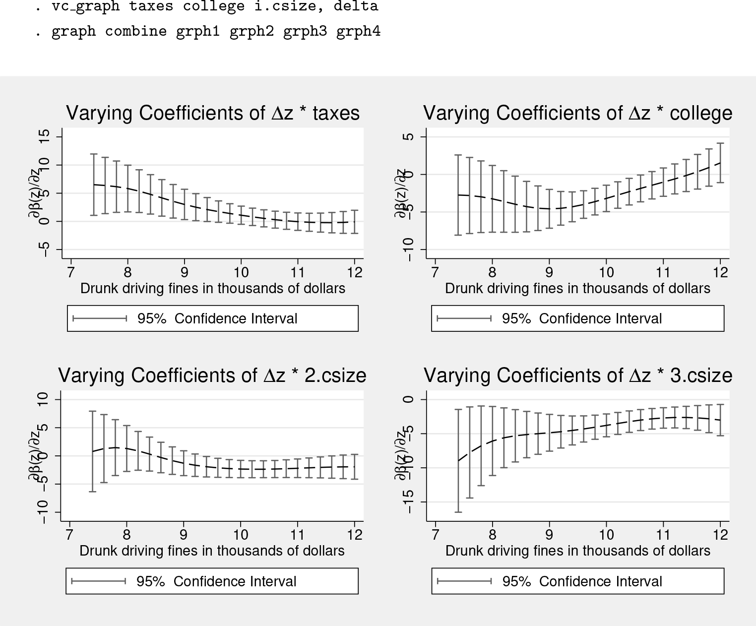
SVCM: Change of the conditional effects across fines ∂β(z)/∂z
An interpretation of these results can be given as follows. Overall, when alcoholic beverages are taxed, the number of monthly citations per month decreases by 4.5 units (table 1 column 1). This effect is larger in jurisdictions with low fines, with a point estimate ranging from 15 to just below 4, and in jurisdictions with fines levels above 10. No differences can be observed in the conditional effect for fine levels above 10. This is mirrored by the fact that the estimate of ∂β(z)/∂z in figure 3 is statistically equal to zero.
If there is a college campus in town, the number of citations per month is about 5.8 higher. The conditional impact of college declines as fines increase by almost 10 points between the minimum and maximum levels of fines in the distribution. Based on the estimates from figure 3, when fines are above 11, the change in the effect of college on citations is no longer statistically significant. If the jurisdiction is located in a medium city, the impact on the number of citations is relatively small and statistically significant but shows no statistically significant change across fines. Finally, if the jurisdiction is located in a large city, the conditional impact is large, ranging from 10 to 30 additional citations per month, declining as fines increase. Note from these figures that most estimates for fines under 9 show large confidence intervals because less than 10% of the data fall below this threshold.
5 Conclusions
SVCMs are an alternative to full nonparametric models that can be used to analyze relationships between dependent and independent variables under the assumption that those relationships are linear conditional on a smaller set of explanatory variables. They are less affected by the curse of dimensionality problem because fewer variables enter the estimation nonparametrically. In this article, I reviewed the model selection, estimation, and testing for these types of models and introduced a set of commands,
Supplemental Material
Supplemental Material, st0613 - Smooth varying-coefficient models in Stata
Supplemental Material, st0613 for Smooth varying-coefficient models in Stata by Fernando Rios-Avila in The Stata Journal
Footnotes
6 Programs and supplemental materials
To install a snapshot of the corresponding software files as they existed at the time of publication of this article, type
Notes
A Appendix: Kernel functions and standardized kernel weights
For the following definitions, u = (Zi − z)/h, where Zi is the evaluated point, z is the point of reference, and h is the bandwidth.
References
Supplementary Material
Please find the following supplemental material available below.
For Open Access articles published under a Creative Commons License, all supplemental material carries the same license as the article it is associated with.
For non-Open Access articles published, all supplemental material carries a non-exclusive license, and permission requests for re-use of supplemental material or any part of supplemental material shall be sent directly to the copyright owner as specified in the copyright notice associated with the article.