Causal mediation analysis in instrumental-variables regressions

Abstract

In this article, we describe the use of ivmediate, a new command to estimate causal mediation effects in instrumental-variables settings using the framework developed by Dippel et al. (2020, unpublished manuscript). ivmediate allows estimation of a treatment effect and the share of this effect that can be attributed to a mediator variable. While both treatment and mediator can be potentially endogenous, a single instrument suffices to identify both the causal treatment and the mediation effects.

1 Introduction

There are many settings where a researcher would like to understand the mechanism that underlies an estimated effect of a treatment T on an outcome Y . For example, Becker and Woessmann (2009) are interested in the Weber hypothesis that religion, specifically Protestantism, affects economic growth. Because Protestantism promoted reading of the Bible, ¹ they establish that an underlying mechanism M of the effect of religion on economic growth works through human capital accumulation, especially literacy. Given that the prevalence of religion across regions is likely not random, they introduce an instrumental variable (IV) and show that Protestantism caused higher literacy rates and thus economic growth. They derive plausible bounds for the range of a mediation effect but lack a formal framework to causally estimate the indirect effect of religion on economic growth that works through literacy.

Such an exercise of unpacking mechanisms is called mediation analysis, where a treatment T and one of its outcomes M, that is, the mediator, jointly cause a final outcome of interest Y . Mediation analysis has long been used in settings where T can be assumed to be randomly assigned. However, when T is systematically nonrandom and therefore needs to be instrumented by a variable Z, ² there has been a lack of frameworks for undertaking mediation analysis in such IV settings without having separate instruments for both T and M. ³ The command ivmediate fills this gap and provides a new regression command that allows researchers to use a single IV to estimate the causal effect of the intermediate variable on a final outcome using the estimator developed by Dippel et al. (2020). This complements existing ways to estimate causal mediation effects that assume randomness in the assignment of treatment T (Imai, Keele, and Tingley 2010) or require separate instruments for T and M (for example, Frölich and Huber [2017]; Jun et al. [2016]).

Table 1 illustrates the identification challenge described above. As a starting point, we show the standard IV estimations of the causal effect of T on M (model I) and the causal effect of T on Y (model II). In model I, T is considered endogenous (that is, ${\epsilon }_T\cancel{\coprod }{\epsilon }_M$ ) and we introduce for the endogenous treatment T an IV Z, which is both uncorrelated with the omitted variables (Z ∐ ε_T , ε_M ) and a reasonably strong predictor of T. Model II fits the TE of T on Y using the same IV approach: ${\epsilon }_T\cancel{\coprod }{\eta }_Y$ , but Z is exogenous (that is, $\begin{array}{l}Z\cancel{\coprod }{\epsilon }_T,\hspace{0.17em}{\eta }_Y\\ \end{array}$ ). Table 1 is reprinted from Dippel et al. (2020).

Table 1.

The identification problem of mediation analysis with IV

NOTES: (a) Model I is the standard IV model, which enables the identification of the causal effect of T on M. Model II is the standard IV model that enables the identification of the causal effects of T on Y . Model III is the IV Mediation Model with an instrumental variable Z. (b) Panel A gives the graphical representation of the models. Panel B presents the non-parametric structural equations of each model. Conditioning variables are suppressed for sake of notational simplicity. We use ∐ to denote statistical independence.

To identify what fraction of the TE is explained by the indirect effect, we have to perform a mediation analysis that decomposes the TE of T on Y into 1) the mediated “indirect” effect of T on Y that operates through M and 2) the residual “direct” effect that does not work through M. Model III of table 1 shows the main identification challenge in combining the two IV models into a general mediation model. Equations M = f_M (T, ε_M ) and Y = f_Y (T, M, ε_Y ) imply that T causes Y indirectly through M as well as directly, which is graphically represented by the arrow directly linking T to Y . In a regression of Y on both T and M, there are two potentially endogenous regressors (that is, ${\epsilon }_T\cancel{\coprod }{\epsilon }_Y$ and ${\epsilon }_M\cancel{\coprod }{\epsilon }_Y$ ), but there is only one instrument Z to address this endogeneity.

To overcome the underidentification problem, we do not assume away endogeneity in any of the key relationships in model III ( ${\epsilon }_T\cancel{\coprod }{\epsilon }_M$ , ${\epsilon }_M\cancel{\coprod }{\epsilon }_Y$ , and ${\epsilon }_T\cancel{\coprod }{\epsilon }_Y$ are all maintained), yet we do not need additional instruments. Instead, the omitted variable concerns themselves can suggest a natural solution. This is the case when T is endogenous in a regression of M on T because of confounders that jointly affect M and T and when T is endogenous in a regression of Y on T because of the same confounders that affect Y primarily through M.

Dippel et al. (2020) show that this assumption alone is sufficient to unpack the causal channels in model III, therefore allowing us to identify the extent to which T causes Y through M. Under linearity, the resulting identification framework is straightforward to estimate using three separate two-stage least squares (2SLS) regressions; these estimate i) the effect of T on M, ii) the effect of T on Y , and iii) the effect of M on Y conditional on T .

In the following section, we will briefly explain the underlying econometric theory before we explain the estimation procedure in section 3. There, we also provide further guidance on the interpretation of results and issues regarding weak identification that are typical concerns for applied researchers. Section 4 describes the syntax and options of ivmediate. Section 5 provides a brief simulation exercise in section 5.1 to show not only how ivmediate estimates the correct TE of a treatment but also how these can be decomposed into direct and indirect effects. We then apply the command to a real-life example using the data and empirical setting of Becker and Woessmann (2009) in section 5.2 to estimate how Protestantism affects local economic performance in Prussian counties in 1877 and how much of this effect is causally mediated by literacy.

2 Causal mediation analysis in IV models

Under linearity and with an instrument Z, the causal relations in model III in table 1 can be written as

$Z={\epsilon }_Z$

1

$T={\beta }_T^Z \times Z+{\epsilon }_T$

2

$M={\beta }_M^T \times T+{\epsilon }_M$

3

$Y={\beta }_Y^T \times T+{\beta }_Y^M \times M+{\epsilon }_Y$

4

Equations (1) –(4) can be compactly expressed as X = Ψ × X + ε in (5):

$\underset{\text{x}}{\underbrace{\left[\begin{array}{c}Z\\ T\\ M\\ Y\end{array}\right]}}=\underset{\text{ψ}}{\underbrace{\left[\begin{array}{cccc}0& 0& 0& 0\\ {\beta }_T^Z& 0& 0& 0\\ 0& {\beta }_M^T& 0& 0\\ 0& {\beta }_Y^T& {\beta }_Y^M& 0\end{array}\right]}}\times \underset{\text{x}}{\underbrace{\left[\begin{array}{c}Z\\ T\\ M\\ Y\end{array}\right]}}+\underset{\epsilon }{\underbrace{\left[\begin{array}{c}{\epsilon }_Z\\ {\epsilon }_T\\ {\epsilon }_M\\ {\epsilon }_Y\end{array}\right]}}$

5

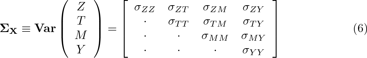
Equation (6) presents the covariance matrix Σ_X of observed variables X:

${\displaystyle \sum {\hspace{0.17em}}_x\equiv \text{Var}}\left(\begin{array}{c}Z\\ T\\ M\\ Y\end{array}\right)=\left[\begin{array}{cccc}{\sigma }_{ZZ}& {\sigma }_{ZT}& {\sigma }_{ZM}& {\sigma }_{ZY}\\ \cdot & {\sigma }_{TT}& {\sigma }_{TM}& {\sigma }_{TY}\\ \cdot & \cdot & {\sigma }_{MM}& {\sigma }_{MY}\\ \cdot & \cdot & \cdot & {\sigma }_{YY}\end{array}\right]$

6

Let Σ _ε denote the covariance matrix of unobserved error terms ε. Because Z is an IV, it implies that ε_Z is statistically independent of ε_T , ε_M , and ε_Y . Thus, Σ _ε is given by

${\sum }_{\in }\equiv \text{Var}\left(\begin{array}{c}{\in }_Z\\ {\in }_T\\ {\in }_M\\ {\in }_Y\end{array}\right)=\left[\begin{array}{cccc}{\sigma }_{\in Z}^2& 0& 0& 0\\ \cdot & {\sigma }_{\in T}^2& {\rho }_{TM}{\sigma }_{\in T}{\sigma }_{\in M}& {\rho }_{TY}{\sigma }_{\in T}{\sigma }_{\in Y}\\ \cdot & \cdot & {\sigma }_{\in M}^2& {\rho }_{MY}{\sigma }_{\in M}{\sigma }_{\in Y}\\ \cdot & \cdot & \cdot & {\sigma }_{\in Y}^2\end{array}\right]$

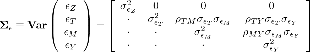
The identifying assumption in Dippel et al. (2020) is that T is endogenous in a regression of Y on T , but endogeneity cannot arise from confounders that jointly influence T and Y , only from confounders that jointly affect T and M (for example, Protestantism and literacy in Becker and Woessmann [2009]). The framework also allows for confounders that jointly influence M and Y (for example, literacy and economic growth in Becker and Woessmann [2009]). Formally, the identifying assumption is ρ_TY = 0 in Σ _ε , while allowing ρ_TM ≠ 0 and ρ_MY ≠ 0.

In section 5.1, we describe how to generate a simulated dataset with these dependent relations.

3 Estimation

3.1 Estimation procedure

The estimation equations to identify all linear coefficients are associated with well-known econometric estimators as follows (control variables are suppressed for notational simplicity and without loss of generality):

1. Parameter ${\beta }_M^T$ is identified by standard 2SLS estimation, described by the following two-equation system:

$\text{First stage}:T={\beta }_T^Z \times Z+{\epsilon }_T$

7

$\text{Second stage}:M={\beta }_M^T \times \widehat{T} +{\epsilon }_M$

8

where $\widehat{T}$ stands for the estimated values of T in the first stage.

2. Dippel et al. (2020) show that the identifying assumption ρ_TY = 0 yields a new exclusion restriction, which allows for the use of Z as an instrument for M when conditioned on T (but not unconditionally). This implies that ${\beta }_Y^M$ and ${\beta }_Y^T$ are the expected values of the estimators of a 2SLS regression where T plays the role of a conditioning variable, Z is the instrument, M is the endogenous variable, and Y is the dependent variable. Namely, ${\beta }_Y^M$ and ${\beta }_Y^T$ can be fit by the following 2SLS model:

$\text{First stage}:M={\gamma }_M^Z\times Z+{\gamma }_M^T\times T+{\epsilon }_T$

9

$\text{Second stage}:Y={\beta }_Y^M\times \widehat{M} +{\beta }_Y^T\times T+{\epsilon }_Y$

10

where $\widehat{M}$ are the estimated values of M in the first stage.

The estimation procedure associated with (7) and (8) is the standard IV approach. By contrast, the estimation procedure associated with (9) and (10) is novel and a property of the framework laid out in Dippel et al. (2020).

There are two first stages here in (7) and (9) for which ivmediate provides tests for weak identification by reporting the corresponding F statistics on the excluded instrument. If robust or cluster–robust standard errors are requested, the regression output displays the F statistic by Kleibergen and Paap (2006). To implement estimation of their corrected F statistic, we rely on the ranktest command by Kleibergen and Schaffer (2007).

In section 5.1, we compare the unbiased estimates resulting from (7)–(10) with the associated OLS estimates.

3.2 Interpretation

There is another explicit link between (7)–(10) and the direct estimation of the TE in model II of table 1. Model II is obtained from model III by substituting (8) into (10):

$\begin{array}{c}Y={\beta }_Y^M\times ({\beta }_M^T\times T+{\epsilon }_M)+{\beta }_Y^T\times T+{\epsilon }_Y\\ =\underset{\text{TE}}{\underbrace{({\beta }_Y^M\times {\beta }_M^T+{\beta }_Y^T)}}\times T+\underset{{\eta }_Y}{\underbrace{{\beta }_Y^M{\epsilon }_M+{\epsilon }_Y}}\equiv g_Y(T,{\eta }_Y)\end{array}$

11

Equation (11) shows that the direct estimate of TE produced by model II is algebraically identical to the product of estimates ${\beta }_Y^T+{\beta }_M^T\times {\beta }_Y^M$ produced by model III [that is, (7)–(10)]. ⁴ This algebraic equivalence holds for a scalar instrument Z, but may not hold with a vector of instruments Z′. The ivmediate command, therefore, is limited to the use of a single scalar instrument. ⁵

It is also worth noting that, in the mediation framework, either ${\beta }_Y^T$ or ${\beta }_M^T\times {\beta }_Y^M$ (but not both) can have opposite signs. For example, there is nothing logically inconsistent about having a positive TE that is composed of a (larger) positive indirect effect that is partly offset by a negative direct effect, or vice versa. In such a case, a statement like “the indirect effect explains more than 100 percent of the total effect” is not incorrect, but it does require careful explanation to avoid confusion.

3.3 Weak identification with two first-stage regressions

Applied researchers are now well aware of the bias introduced by weak identification in an IV setting (Bound, Jaeger, and Baker 1995). A rule of thumb is that an F test of the excluded instrument(s) in the first stage should yield an F statistic of 10 or more (Stock and Yogo 2005). How does this apply to the IV mediation setting with two first stages? Currently, there is no theory to guide applied researchers. Instead, we apply the code from section 5.1 to simulate the behavior of the estimator under different instrument strengths in the treatment and the mediator first stages. This is done by varying the amount of noise in ε_T and ε_Y .

Figure 1 plots the coefficient values of the total, direct, and indirect effects over different values of the first-stage F statistic. The left panel manipulates the strength of the instrument in the treatment first stage, and the right panel manipulates that in the mediation first stage. The instrument is only ever weak in one of the two first stages but not in both at the same time. Samples were simulated according to (1)–(4) with 1,000 observations for each value of the error variance. The values increase from 1 to 15 in increments of 0.5. In the example, the true values of the direct and indirect effects are both 1, summing up to a true TE of 2. The ivmediate simulations were then run 100 times for each error variance value.

Figure 1.

Coefficient values under differing IV strengths in either first stage. NOTE: The left panel simulated data for different values of Var(ε_T ), and the right simulated data for different values of Var(ε_Y ) ranging from 1 to 15. The value of Var(ε_T ) increases in steps of 0.5, and at each step, 100 random samples were drawn according to (1)–(4) with 1,000 observations. Both panels show binned scatter plots of coefficient values of the total, direct, and indirect effects over different values of the corresponding first-stage F statistics where the strength of the instrument was manipulated. The true TE is 2, and the true direct and indirect effects are equal to 1.

The left panel shows that, as the treatment first-stage F statistic approaches the rule of thumb value of 10, all effects begin to center on their true values. This is also the case for the right panel, however, here the direct effect takes longer to center on its true value. It only begins to center on the true value from a mediation first-stage F statistic of 30. A conservative approach would therefore require a stronger instrument in the mediator first stage to accurately identify all three effects. If interest only lies on the indirect effect, the commonly used approximation rule for a reasonably strong instrument seems applicable.

4 The ivmediate command

4.1 Syntax

ivmediate depvar [indepvars] [if] [in] [, mediator( varname ) treatment( varname ) instrument( varname ) absorb( varname ) full vce( vcetype ) level( # ) ]

4.2 Description

ivmediate implements the causal mediation analysis framework for IV models introduced by Dippel et al. (2020). The command allows the estimation of the causal treatment and mediation effects for potentially endogenous treatment and mediator variables without the need for an additional instrument for the mediator. A single IV suffices to identify both effects.

4.3 Options

mediator( varname ) includes a single mediator variable. mediator() is required.

treatment( varname ) includes a single treatment variable. treatment() is required.

instrument( varname ) includes a single IV. instrument() is required.

absorb( varname ) allows the absorption of one fixed effect. For details, see [R] areg.

full displays intermediate results together with the main results. Specifying this option will display three intermediate output tables:

the IV regression of Y on T (instrumented with Z)

the IV regression of M on T (instrumented with Z), for which the first-stage F statistic is reported as first stage one in the main table

the IV regression of Y on M (instrumented with Z) and controlling for T, for which the first-stage F statistic is reported as first stage two in the main table

The TE is the coefficient on T in the first table; the direct effect is the coefficient on T in the third table; the indirect effect is the product of the coefficient on T in the second table and the coefficient on M in the third. The mediation effect as percentage of the TE is therefore the indirect effect divided by the TE times 100.

vce( vcetype ) may be robust to estimate Eicker/Huber/White standard errors or may be cluster clustervar to estimate cluster–robust standard errors. The default is vce(unadjusted) standard errors.

level( # ) specifies the confidence level, as a percentage, for confidence intervals. Integers between 10 and 99 inclusive are allowed. The default is level(95) or as set by set level; see [U] 20.8 Specifying the width of confidence intervals.

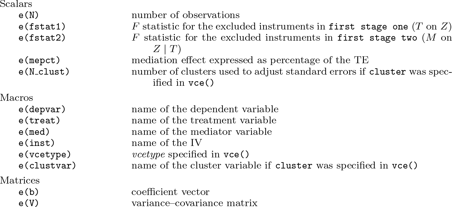
4.4 Stored results

ivmediate stores the following in e():

Empirical example

5.1 Simulation exercise

A simulated dataset with the assumed dependent relations can be straightforwardly generated in the following way:

Separately generate error terms ε_T and ε_Y that are normally distributed with mean 0 and variance 1, N(0, 1). These are statistically independent, that is, ε_T ∐ ε_Y .

Let error term ε_M be defined as ${\epsilon }_M=\sqrt{\omega }\times {\epsilon }_T+\sqrt[\hspace{0.17em}]{(\text{1}-\omega )}\times {\epsilon }_Y$ for any ω ∊ [0, 1]. ⁶

The correlation between ε_M and ε_T is given by ${\rho }_{TM}=\sqrt{\omega }$ . Thereby, ${\epsilon }_M\cancel{\coprod }{\epsilon }_T$ . By symmetry, we also have that ${\rho }_{MY}=\sqrt{(\text{1}-\omega )}$ and ${\epsilon }_M\cancel{\coprod }{\epsilon }_Y$ . Having drawn ε_T and ε_Y independently implies that the correlation between ε_T and ε_Y is ρ_TY = 0. However, conditioning on ε_M = e induces a linear relation between ε_T and ε_Y , namely, ${\epsilon }_T=e/\sqrt{\omega }-\sqrt{(\text{1}-\omega )/\omega }\times {\epsilon }_Y$ . Thus, the correlation between ε_T and ε_Y conditioned on ε_M is ρ_{TY |} εM = −1 and, thereby, ${\epsilon }_T\cancel{\coprod }{\epsilon }_Y|{\epsilon }_M$ . A high ω implies a high ρ_TM . By contrast, a low ω implies a high ρ_MY .

It is instructive to investigate the bias generated by a misspecified model where T and M are assumed to be exogenous, that is, the mutual independence of ε_T , ε_M , and ε_Y is wrongly assumed. Let the data be generated by (1)–(4) and the model coefficients be normalized to equal 1, that is, ${\beta }_T^Z={\beta }_M^T={\beta }_Y^T={\beta }_Y^M=\text{1}$ . The true parameters ${\beta }_M^T,{\beta }_Y^T$ , and ${\beta }_Y^M$ are identified through (7)–(10). If the error terms ε_T , ε_Y , and ε_M were wrongly assumed to be statistically independent, then parameters ${\beta }_M^T,{\beta }_Y^T$ , and ${\beta }_Y^M$ could be estimated by OLS through the following equations:

$\begin{array}{l}\text{OLS}:{\beta }_M^T=\frac{{\sigma }_{TM}}{{\sigma }_{TY}}\\ \text{OLS}:{\beta }_Y^T=\frac{{\sigma }_{MM}{\sigma }_{TY}-{\sigma }_{TM}{\sigma }_{MY}}{{\sigma }_{MM}{\sigma }_{TT}-{\sigma }_{TM}^2}\\ \text{OLS}:{\beta }_Y^M=\frac{-{\sigma }_{TM}{\sigma }_{TY}-{\sigma }_{TT}{\sigma }_{MY}}{{\sigma }_{MM}{\sigma }_{TT}-{\sigma }_{TM}^2}\end{array}$

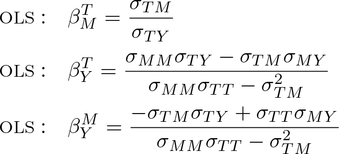
While the true parameters are set to be 1, the OLS estimators may range from 0 to 2 depending on the error correlations. Because a high ω implies pronounced bias in the relation between T and M (a high ρ_TM ), the OLS estimate of ${\beta }_M^T$ diverges from the true value 1 as ω increases. By contrast, the OLS estimates of ${\beta }_Y^T$ and ${\beta }_Y^M$ converge to the true value 1.

Given the model parameters, the TE of ${\beta }_Y^M\times {\beta }_M^T+{\beta }_Y^T=\text{1}\times \text{1}+\text{1}=\text{2}$ is not recovered by simple OLS. In fact, not even the 95% confidence interval would include the true TE. On the other hand, 2SLS did recover the TE, but it could not disentangle the direct effect of the treatment (net of the mediator) from the indirect effect of the mediating variable. The simulation shows how ivmediate can both recover the true TE and decompose it into the direct and indirect effects as described in the theoretical section.

5.2 Applied example using the Becker and Woessmann (2009) data

The example below uses data from Becker and Woessmann (2009), who estimate the effect of Protestantism on economic prosperity in Prussian counties. To obtain exogenous variation in the share of Protestants in these counties, they used the fact that Protestantism spread concentrically around Wittenberg, the city where Martin Luther taught and preached. Following their example, we use distance to Wittenberg (kmwitt) as an instrument for the share of Protestants (f_prot) with the outcome being the per capita income tax (inctax) in 1877 as a measure for economic performance. The mediator we consider is the share of literate population (f_rw).

According to Becker and Woessmann (2009), Protestantism promoted reading of the Bible, which led to human capital accumulation and therefore promoted economic development. They are interested in estimating

$Y=\alpha \text{Prot}+\chi \text{Lit}+X^{\prime }\gamma +\epsilon$

12

though they note that the “problem with such a model is that not only Protestantism but also literacy may be endogenous in this setting” (p. 570). Because they have no additional instrument for literacy, they use different types of bounding exercises using estimates from previous literature on the returns to education (see section VI.C in the original study). Using ivmediate, we can go further and directly estimate the mediation effect of literacy that goes through Protestantism with only one instrument.

As in the original study, we condition on further covariates in the estimation of (12), which are the share of Jewish population, female population, individuals aged below 10, the share of population of Prussian origin, average household size, population size of the county, the percentage population growth between 1867 and 1871, and the share of the population with missing information on literacy. ⁷

The TE estimates that every 1 percentage point increase in the share of Protestants increases per capita income tax revenues by 0.83 Marks. Under the typical IV assumptions, this effect is causal. The direct effect estimates that only 0.08 Marks of this increase are because of Protestantism itself and it is not statistically significant. However, the indirect effect estimates that 0.75 Marks of this increase are caused by literacy as a mediating factor. This implies that literacy explains 90% of the TE of Protestantism on economic outcomes. This is in line with the findings by Becker and Woessmann (2009), who conclude that “Protestants’ higher literacy can account for roughly the whole gap in economic outcomes between the two denominations [Catholics and Protestants]” (p. 576).

Supplemental Material

Supplemental Material, st0611 - Causal mediation analysis in instrumental-variables regressions

Supplemental Material, st0611 for Causal mediation analysis in instrumental-variables regressions by Christian Dippel, Andreas Ferrara and Stephan Heblich in The Stata Journal