Sage Journals: Discover world-class research

Abstract

In this article, we introduce a new command, sfcount, to fit count-data stochastic frontier models. Although originally designed to estimate production and production-cost functions, this new command can be used to estimate mean regression functions when count data are suspected to be underreported or over-reported.

Keywords

st0607 sfcount stochastic frontier underreporting overreporting lowdiscrepancy series mixed Poisson distribution Poisson log-half-normal model maximum simulated likelihood

1 Introduction

In this article, we introduce a new command, sfcount, that estimates the parameters of the count-data stochastic frontier model in Fé and Hofler (2013).

Stochastic frontier models (Aigner, Lovell, and Schmidt 1977; Meeusen and van den Broeck 1977) are central to the identification of inefficiencies in the production (and production costs) of continuously distributed outputs. In labor, industrial, and health economics, production frontiers have also been adopted to explain deviations from maximum or minimum levels of nontangible and nonpecuniary outcomes. However, in these latter domains, outcomes are often measured as counts (for example, the number of patents obtained by a firm or the number of infant deaths in a region). Although these latter fields of inquiry have not emphasized the idea of inefficiency in the “production” of nontangible and nonpecuniary outcomes, recent contributions (for example, Fé [2013]; Fé and Hofler [2013]) suggest that inefficiencies are also present in these domains.

The need for specific count-data models for stochastic frontiers arises because this results in more efficient estimation (for example, Greene [2018]) and, more critically, inefficiency is typically not nonparametrically identified from data alone. Therefore, researchers have to make specific assumptions regarding the distribution of inefficiency in the sample or the population. These assumptions define the class of admissible distribution underlying outcomes. Standard continuous data models attribute any negative (positive) skewness in the sample to inefficiencies in the production of economic goods (bads). However, the distributions of discrete outcomes are typically skewed even in the absence of inefficiencies (for example, the Poisson distribution), and the sign of skewness is generally independent of whether one is studying an economic good or an economic bad. Thus, standard stochastic frontier models can fail to detect any inefficiency in production when the outcome of interest is a count—even when the underlying inefficiency is substantial.

The core count-data stochastic frontier model is based on a mixed Poisson distribution with a log-half-normal mixing parameter (or a Poisson log-half-normal [PHN] in the parlance of Fé and Hofler [2013]). Although the motivation behind this model was the estimation of stochastic frontiers under discrete valued outcomes, the PHN can be used for modeling underreported counts as well as overreported counts. These situations are pervasive when studying worker’s absenteeism (Winkelmann 1996), consumer data (Fader and Hardie 2000), drug abuse (Brookoff, Campbell, and Shaw 1993), or traffic accidents (Alsop and Langley 2001), among others. Among the models traditionally used for modeling these events, the beta-binomial and Poisson-lognormal models have been widely used. The PHN is a complement to these specifications.

The code presented here extends the catalog of Stata commands pertaining to the stochastic frontier literature, including the original Stata commands frontier and xtfrontier as the recent extensions sfcross and sfpanel by Belotti et al. (2013). The original model in Fé and Hofler (2013) was cross-sectional. Therefore, this code does not account for individual time-invariant heterogeneity. In the continuous outcome stochastic frontier literature, panel-data extensions abound. For an excellent review— including extensions—see Greene (2005); a recent important methodological contribution is Belotti and Ilardi (2018). Similarly, the original model in Fé and Hofler (2013) did not deal with endogenous regressors. This is an active area of research in the general stochastic frontier literature. Seminal contributions include Kutlu (2010), Griffiths and Hajargasht (2016), and Amsler, Prokhorov, and Schmidt (2016).¹ The development of a count-data model with covariates endogenous to inefficiency is an unexplored area of work.

2 Methods

To introduce the PHN model, we adopt the stochastic frontier terminology in Fé and Hofler (2013). The relationship to underreported or overreported count models will be apparent from the context. There is a sample of i = 1,…, n units containing data on a discrete outcome of interest y_i ∊ {0, 1, 2,…}. The mean production frontier of y is determined by the mapping

log \tilde{λ} = h (x; β)

where $\tilde{λ} \in ℝ^{+}$ . Conditional on a level of inefficiency (or level of underreporting or overreporting) ε ∊ ℝ⁺, the mean deterministic frontier is

log λ = h (x; β) \pm ε

Because we are modeling nonnegative count data, we transform the last equation to

λ = exp {h (x; β) \pm ε}

Following convention, we assume that y has a Poisson distribution conditional on a set of regressors, x, and ε, with λ as the conditional mean of the distribution. The unconditional distribution follows by endowing ε with a specific density. Following the convention in the stochastic frontier literature, Fé and Hofler (2013) assume that ε follows a half normal distribution, so that

f (ε) = f (ε; σ) = \frac{2}{σ \sqrt{2 π}} \exp (- \frac{ε^{2}}{2 σ^{2}}) Ι_{[0, \infty)} for σ_{ε} > 0

This density has the advantage of allowing some flexibility, thanks to its scale parameter. It also leads to a model whose first-order moments are well defined (a property that is not shared by some popular distributions).²

If f(ε) is half normal, we can write ε = |u|, where u has a normal distribution. With this notation, and letting h(x; β) = x ′β, the conditional distribution of y given x follows by averaging ℙ(y| x , u) over the range of u,

\begin{array}{l} ℙ (y | X; σ, β) = E (\frac{[exp {- exp (X^{'} β \pm σ | υ |)}] exp {y (X^{'} β \pm σ | υ |)}}{y!}) \\ = E [Poisson {exp (X^{'} β \pm σ | υ |)}] \end{array}

where expectations are taken with respect to the standard normal distribution. Fé and Hofler (2013) provide expressions for the moments of f(ε) when this follows a halfnormal density function, as well as expressions for the conditional mean and variance of y. The PHN distribution does not have a closed-form expression; however, the integral in (2) can be approximated by simulation. Specifically, Fé and Hofler (2013) advocate combining maximum simulated likelihood (MSL) estimation of the PHN model with Halton sequences (Gentle 2003). Applying simulation, we approximate the conditional distribution of y_i (for i = 1,…, n) by the sum

ℙ (y | X; θ) \approx \overset{⌢}{ℙ} (y | X; s_{h}, θ) = \frac{1}{H} \sum_{h = 1}^{H} Poisson {exp (X^{'} β \pm σ | s_{h} |)}

where θ′ = (β′, σ) and s_h are the terms of a Halton sequence, possibly randomized.

The infeasible log likelihood $L_{n} = \sum_{i = 1}^{n} l o g ℙ (y | x; θ)$ can be approximated by $\sum_{i = 1}^{n} l o g \overset{⌢}{ℙ} (y | x; s_{h}, θ)$ . The analytical derivatives of Ln,h are given by

\frac{\partial L_{n, h}}{\partial θ} = \sum_{i = 1}^{n} \frac{1}{\overset{⌢}{ℙ} (y_{i} | X_{i}; s_{h}, θ)} \frac{1}{H} \sum_{h = 1}^{H} Poisson ({\tilde{λ}}_{i, h}) (y_{i} - {\tilde{λ}}_{i, h}) {\begin{matrix} X_{i} \\ \pm | s_{h} | \end{matrix}}

where ${\tilde{λ}}_{i, h} = \exp (X_{i}^{'} β \pm σ | s_{h} |) .$ The value ${\overset{⌢}{θ}}_{M S L}$ making the above system of equations equal to zero is the MSL estimator of θ. When the PHN is a correct representation of the underlying data-generating process, ${\overset{⌢}{θ}}_{M S L}$ is a consistent, asymptotically normal and efficient estimator of the true parameter value, as follows from properties (1) and (2) above. Standard errors can be computed via the Berndt–Hall–Hall–Hausman estimator or the minus inverse of the Hessian matrix of L_n,h .

Tests of hypotheses can rely on the Wald score likelihood-ratio trinity. Testing the null hypothesis of no inefficiency is of particular interest. The null hypothesis would be

H_{0} : σ = 0

in which case PHN collapses to a standard Poisson model. A formal test can be computed via a likelihood ratio comparing the resulting value with the quantiles of a χ1² distribution.

2.1 Estimating cross-sectional inefficiency

Although the parameters of the frontier are of interest in themselves, the ultimate goal of most stochastic frontier analyses is to obtain approximate efficiency scores (that is, measures of the deviations away from either maximum or minimum values of the outcome) for each individual in the sample. Following Jondrow et al. (1982) cross-sectional inefficiency scores, we can estimate v = exp(±|u|) via E(v|y, x). Using Bayes’s theorem, we see

\begin{array}{l} f (v | X, y) = \frac{ℙ (y | X, v) f (v)}{ℙ (y | X)} \end{array}

so that

E (v | y,X) = \int v f (v | X, y) d v

The latter expression does not have a closed form. However, we may still approximate the relevant integral via simulation. The simulated E(v|y, x) for the parametric mixed Poisson model is

{\hat{v}}_{i} = E (v_{i} | X_{i}, y_{i}) \approx \frac{\sum_{h = 1}^{H} \exp (\pm | s_{h} | σ) Poisson {\exp (X_{i}^{'} β + σ | s_{h} |)}}{\sum_{h = 1}^{H} Poisson {\exp (X_{i}^{'} β + σ | s_{n} |)}}

Two remarks are important here. First, the distributions of v and $\hat{v}$ are not the same,³ and the lower and upper tails of the distribution of v will be misreported. From a stochastic frontier perspective, this means that $\hat{v}$ penalizes outstanding firms and rewards the least efficient individuals—although the average efficiency in the sample is correctly approximated. However, the estimator is unbiased in the unconditional sense $E (\hat{v} - v) = 0$ (Wang and Schmidt 2009).

Second, in applications, the scores depend critically on the term Poisson{exp(x i′β+ σ|s_h|)}. If the mean of this distribution, exp(x i′β + σ|s_h|), is too large in relation to Y for any one observation, then Poisson{exp(x i′β + σ|s_h|)} will be approximately 0. Therefore, for that observation, the cross-sectional estimate of inefficiency will be 0/0, which Stata reports as a missing value. We thus recommend researchers ensure that the explanatory variables are measured in meaningful units, albeit of small magnitude.

3 The sfcount command

3.1 Syntax

sfcount depvar indepvars [if] [in] [, draws( # ) technique( string ) cost

cluster( string ) vce( vcetype )]

where depvar is the dependent variable and indepvars are the explanatory variables.

3.2 Options

draws( # ) specifies the number of Halton draws. The default is draws(200). The model is fit via MSL. To approximate the likelihood function of the Poisson log-half-normal model, the command uses Halton sequences (a low-discrepancy sequence). Halton sequences ensure a good coverage of the unit interval (for example, Niederreiter [1992]).

technique( string ) specifies the optimization technique. The default is technique(nr), which is the modified Newton–Raphson. You can switch between dfp (Davidon–Fletcher–Powell), bhhh (Berndt–Hall–Hall–Hausman), and bfgs (Broyden–Fletcher–Goldfarb–Shanno).

cost specifies that the underlying model is a cost function (or, equivalently, an overreporting or deviation above the minimum-level function). By default, sfcount estimates a production function (or, equivalently, an underreporting or deviation below the maximum-level function).

cluster( string ) specifies the name of a variable that creates intragroup correlation, relaxing the usual requirement that the observations be independent.

vce( vcetype ) specifies how the variance–covariance matrix of the estimators is to be calculated. Allowed values are the following:

The default is vce(oim), except for technique(bhhh), where it is vce(opg). If cluster() is used, the default becomes vce(robust).

3.3 Cross-sectional estimates of inefficiency

The command automatically generates a variable named inefficiency collecting the cross-sectional scores.

3.4 Example: Stochastic frontier

For this example, we generated 1,000 observations from a PHN distribution with mean exp(1 + x ₁ + x ₂ − v), where x_j ∼ uniform[0, 1] and v has a half-normal distribution with σ = 1 (the code to generate the data appears in the discussion of the Monte Carlo simulation below). This yielded the following output:

The output follows standard Stata convention. The first block of results, eq1, presents the estimates of the structural coefficients of the regressors (including an intercept). The second block of results, eq2, presents the estimate of log(σ). Therefore, the point estimate of σ can be retrieved by using the transformation σ = exp(_cons) in eq2. Below the table of main results, one finds the likelihood-ratio test for H ₀ : σ = 0. In this case, the statistic equals 321.68 with associated p-value of 0.00 (and thus one would reject the null hypothesis).

sfcount automatically calculates the cross-sectional inefficiency scores and stores them in a new variable, inefficiency. The following summary statistics compare the average and actual estimated inefficiencies.

The variable ehat collects the true inefficiency scores, whereas the second variable, inefficiency, collects the estimated inefficiency scores. It is clear that, as Wang and Schmidt (2009) point out, the cross-sectional estimator is unbiased in an unconditional sense; thus, it provides very accurate estimates of the average inefficiency. Even though figure 1 reveals a discrepancy between the actual and the estimated scores (which is expected because, in this simulation, x_j do not provide any information about the inefficiency parameter), there is also a strong positive correlation between the actual and estimated inefficiencies. The smaller standard deviation (SD) in the estimated inefficiencies is due to $\hat{v}$ being a shrinkage of v toward its mean (as Wang and Schmidt[2009] note).

Figure 1.

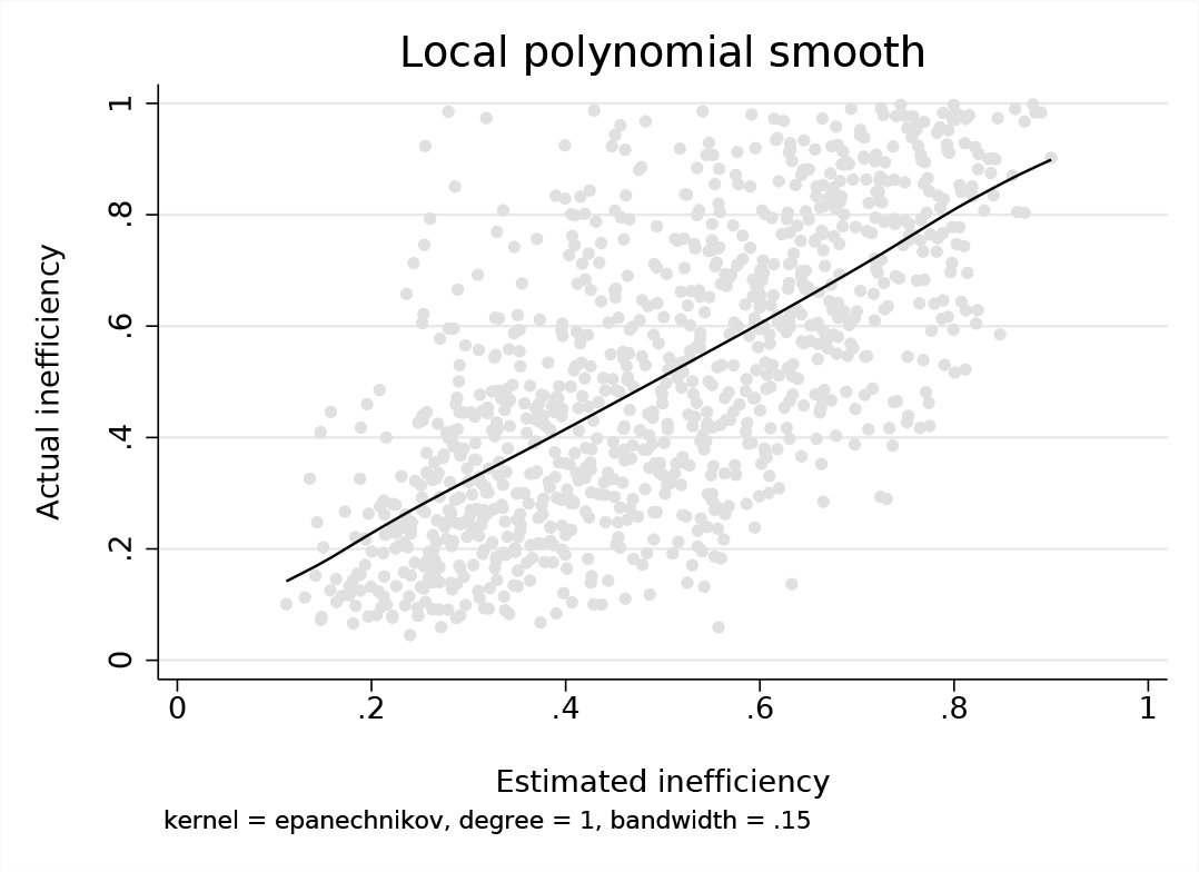
Real versus estimated cross-sectional inefficiency

4 Monte Carlo simulation

To verify the properties of the method and the robustness of the software, we run a Monte Carlo simulation. We drew samples of 100 observations from a PHN model with conditional mean exp(1+x ₁ +x ₂ −σv), where x_j ∼ uniform[0, 1] and v has a half-normal distribution with σ ∊ {0.5, 1, 2}. We estimated the parameters of this model 500 times. We wrote a short ado-file, mc1, to generate the data, fit the model, and return the result to Stata’s simulate command.⁴ The results of each experiment are presented now. For σ = 0.5, we obtained the following results.

Here b0 corresponds to the intercept, b1, b2 are the coefficients of x1, x2, respectively, s is the estimate of σ, and reject is the proportion of times the null hypothesis σ = 0 was rejected by the likelihood-ratio test. We observe that, even for the very small sample size considered, the parameters of the model are very accurately estimated on average. Specifically, the critical parameter σ was tightly concentrated around the true value of 0.5. The empirical power of the likelihood-ratio test was 65%, which is acceptable given the small sample size. Similar conclusions were reached with the alternative specifications.⁵

What would occur if the standard normal–half-normal model in Aigner, Lovell, and Schmidt (1977) were fit to these data instead? We illustrate the situation through a simulation for both the cost and production frontier cases. We maintain the same design but we will focus on the case σ = 1 for simplicity. Following convention in Aigner, Lovell, and Schmidt (1977), we fit the model

log y = θ_{0} + θ_{1} log x_{1} + θ_{2} log x_{2} \pm u + v

where now, u is the inefficiency term (distributed half-normal) and v is the idiosyncratic, zero-mean error term. The case +u corresponds to the cost function, whereas the case −u corresponds to the production frontier. The code to run this simulation is similar to mc1.ado; however, sfcount is replaced by the built-in command frontier, and the variables are transformed to logs. The critical parameters in this model are the standard errors of u and v, say σ_u, σ_v . Specifically, the ratio λ = σ_u/σ_v is the commonly used measure of the magnitude of inefficiency in the sample. In addition to this, the likelihood-ratio test of σ_u = 0 serves, as before, as the statistic to draw inferences regarding the statistical significance of inefficiency in the sample. The result of this is

The critical quantities in the simulation are k3 and s (which corresponds to the ratio λ = σ_u/σ_v ). The production stochastic frontier model expects negative skewness in the log of the dependent variable, and on this occasion, the average skewness happens to be negative (but this is not always the case, as illustrated below). Indeed, the type of skewness exhibited by log Y will depend on the specific parameterization of the generating process (note that the untransformed data will always have a positively skewed distribution). The most critical aspect of these results is that the parameter λ is estimated very imprecisely. The large value of the estimated parameter suggests that too often the model cannot separate inefficiency from pure noise and that all the variation in the sample is erroneously attributed to inefficiency. In contrast, the likelihood-ratio test rejects the null hypothesis only about 70% of the time. The results for the cost frontier are similarly worrying:

In this case, maximum likelihood failed to converge in two replications. As with the production frontier case, the parameter λ is imprecisely estimated (because all variation tends to be attributed to inefficiency). Yet, paradoxically, the significance of the inefficiency term is rejected only about 38% of the time. The critical aspect of this result is that although the distribution of log Y has the right type of skewness (positive), its magnitude is very small; therefore, the cost stochastic frontier model fails to identify any inefficiency, even though this is prevalent in the data.

An even more problematic example arises when we let σ = 3 and try to estimate a production frontier. Here the skewness of log Y is positive, which presents a violation of one of the assumptions underlying the continuous-data stochastic frontier model. In this instance, the latter method fails to detect any inefficiency at all:

As seen from the above results, the likelihood-ratio test rejects the null hypothesis at the nominal 5% level, whereas λ remains imprecisely estimated.

In summary, the continuous-data stochastic frontier model can be problematic in practice when data are coming from the PHN specification.

5 Example: The distribution of infant deaths in England

We next illustrate the use of the sfcount command in practice. Specifically, we model the conditional distribution of infant deaths in England during 2015 and 2016. The help file accompanying the sfcount command details how to reproduce the results of this exercise.

Infant deaths have a large opportunity cost for societies and constitute a marker of the overall health status of a population. Commonly cited risk factors are parental risk behavior, pollution, economic deprivation, and the quality of health providers, although a large proportion of infant deaths are not attributable to any specific cause (and are cataloged as sudden infant death syndrome). It is unclear, however, if the latter deaths still show systematic variation across different areas even after accounting for the effect of measurable determinants of infant deaths. The PHN can help us to detect which areas overreport infant deaths conditional on the area’s characteristics (that is, which areas are inefficient in the production of infant deaths).

To illustrate the workings of the PHN when addressing this question, we downloaded data on infant deaths by local area for the years 2015 and 2016 from the website of the UK Office for National Statistics. We complemented these data with information on local area characteristics from the 2011 UK Census. The focus of the analysis in this exercise is socioeconomic status and air quality. Socioeconomic status has been shown to correlate with health and wealth. Air pollutants can induce respiratory disease (including bronchitis, pneumonia, allergies, or asthma). Among these pollutants, nitrogen oxides (by-products of fuel consumption and the production of electricity) are thought to be important determinants of respiratory diseases.

We proxy each area’s socioeconomic status with, first, the number of people claiming income benefits per 1,000 of the population and, second, the area’s employment rate. Low birthweight is a risk factor for infant mortality; therefore, in our model we also incorporate the percentage of babies born at a gestational age of greater than or equal to 37 weeks and with a birthweight of less than 2,500g. Our indicator of air quality is the area’s average nitrogen oxide emissions intensity score, NO _x . This is an 8-point scale with higher scores indicating higher emissions. We found a few discrepancies between the names and geographic boundaries in the 2011 UK Census and the Office for National Statistics’ most recent data files containing the counts of infant deaths. Given the limited scope of this example, we opted to discard those areas for which data on the covariates were not available for that reason. This leaves us with full data for 309 local areas. For the purposes of this analysis, we pooled the 2015 and 2016 data, while areas’ characteristics were imputed from the 2011 Census.

Descriptive statistics of our limited sample are provided in table 1. The average number of deaths across England was 6.9; however, the distribution is skewed, with a long right tail, as can be seen in figure 2 (the maximum number of deaths observed was 62, in the city of Manchester; note that London has been disaggregated in 31 subareas). The average population in each area is 139,680 inhabitants, whereas the average proportion of underweight births is 7.2%. On average, 12.9% of the population was claiming income benefits, whereas the average employment rate was 77%. The average NO _x score in the sample was 4.1. However, variation is vast, ranging from 1.1 to 8.

Table 1.

Descriptive statistics

	Mean	SD	Min	Max
Number of infant deaths	6.945	7.054	0	62
Nitrogen oxide emissions score	4.144	1.649	1.143	8
Underweight births	7.180	1.323	2.800	11.60
Population	139680.0	83175.8	24457	715402
Employment rate	76.82	3.992	64.73	84.45
Year 2016	0.500	0.500	0	1
East of England East Midlands	0.149 0.129	0.356 0.336	0	1
London	0.100	0.301	0	1
North East	0.0324	0.177	0	1
North West	0.120	0.325	0	1
South East	0.214	0.410	0	1
South West	0.107	0.309	0	1
West Midlands	0.0874	0.283	0	1
Yorkshire and the Humber	0.0615	0.240	0	1
N		618	0	1

Figure 2.

Distribution of infant deaths in England. Years 2015 and 2016.

Before undertaking our analysis, and in view of the results presented in section 4, we studied the empirical distribution of the logarithm of the count of infant deaths. This variable would be sitting at the core of any stochastic frontier analysis using the benchmark continuous-data models (for example, the normal–half-normal model). The mean of this variable is based on 584 observations instead of 618 (5.5% of the areas report 0 deaths) and equals 1.642. Importantly, its skewness equals −0.0444. Parametric cost stochastic frontier models, however, expect the dependent variable to exhibit positive skewness. Indeed, the distribution of the log-deaths variable does not seem to be skewed at all, and a standard test of normality based on the third and fourth moments of the variable did not reject the null hypothesis (sktest; p-value 0.5883). Therefore, data do not seem to support the premises of standard continuous-output stochastic frontier models. This suggests that a standard continuous-data frontier model will not provide a good fit for this variable, as already discussed in section 4. Unsurprisingly, the normal–half-normal model struggled to converge to a solution (because of a “not concave likelihood”).

Having discarded the continuous-data stochastic frontier model, we proceeded to fit a battery of PHN models under nested conditioning sets. Table 2 presents the estimated coefficients of these models. As expected, population size is an important determinant of infant deaths, with larger populations seeing a higher number of deaths. Importantly, we observe that socioeconomic status is negatively associated with infant deaths. Specifically, higher employment rates are strongly associated with a lower count of deaths; however, we found that income benefits and infant deaths are negatively correlated. However, the significance of this contradictory result is sensitive to the structure of the model, which casts some doubts about the reliability of this finding. We did not find any significant association between low birthweight and infant deaths. The most striking result, however, is the very strong association between air pollution and infant deaths. Specifically, higher levels of nitrogen oxides are associated with higher infant deaths.

Table 2.

PHN model (conditional mean)

	(1)	(2)	(3)	(4)
Log population	0.396*** (6.16)	0.357*** (5.74)	0.248*** (4.30)	0.268*** (4.82)
Underweight births		0.0391 (1.25)	0.0111 (0.41)	−0.00691 (−0.26)
Income bene_claimants (per 1000 pop.		−0.0281*** (−3.44)	−0.0178∗ (−2.42)	−0.0185∗ (−2.56)
Employment rate		−0.0968*** (−13.00)	−0.0582*** (−7.77)	−0.0656 (−7.96)
NO_x			0.245*** (14.20)	0.255*** (11.80)
Year 2016 indicator				0.0499 (1.01)
Intercept	−3.901*** (−5.14)	4.245*** (4.73)	1.731∗ (2.11)	2.092∗ (2.37)
Regional indicators	−	−	−	−
log	0.135_(3.08)	−0.0822 (−1.82)	−0.277*** (−6.00)	−0.377*** (−7.12)

NOTES: t statistics in parentheses.

∗ p < 0.05, ∗∗ p < 0.01, ∗∗∗ p < 0.001

All models except (2) return a statistically significant log σ, which suggests that there is substantial “inefficiency” in the sample in the form of higher levels of deaths given the levels predicted by our model. Table 3 summarizes the estimated inefficiency in each of the nine constituent areas. The average value of νb for the whole sample is 1.9. There is substantial variation across regions. Inefficiency is lowest in the West Midlands (1.8). However, while the average estimated inefficiency score for most other regions sits at 1.8–1.9, the estimated inefficiency score for Yorkshire and the Humber is 2.3. Yorkshire and the Humber has the second-largest employment rate in the sample and the second-lowest NO _x emissions score; however, it has the relatively highest level of benefit claimants and underweight births. Given the prominence of employment rate and NO _x scores in our model, it would appear that Yorkshire is underperforming compared with other equally well-off areas of England. In particular, this area seems to exhibit levels of infant death that more than double their predicted levels, given the area’s socioeconomic and environmental credentials.

Table 3.

Inefficiency by region

	Mean	SD	Min.	Max.
East of England	1.937	0.763	1.152	5.479
East Midlands	1.849	0.533	1.278	3.552
London	1.913	0.672	1.113	3.699
North East	1.791	0.451	1.268	2.723
North West	1.921	0.838	1.149	6.461
South East	1.903	0.720	1.195	6.158
South West	1.870	0.596	1.300	4.320
West Midlands	1.753	0.427	1.255	3.132
Yorkshire and the Humber	2.302	1.516	1.256	6.227
Total	1.908	0.755	1.113	6.461

We conclude this illustration of the sfcount command in practice with two caveats regarding the preceding application. Some significant limitations restrict the scope and interpretation of the results. First, the model captures association only between the dependent and independent variables. In particular, we fall short of making any causal claims, especially in view that deaths, socioeconomic status and air quality might be either jointly determined or influenced by common unmeasurable factors. These factors might also determine the amount of inefficiency in the data. Second, we have considered a very limited number of explanatory variables, and these were imputed from past observations. Thus, there is a considerable risk that our results are driven by latent heterogeneity; in addition measurement error is likely to bias our results away from any causal parameter. Ultimately, however, the preceding analysis must be understood within the context of an illustration of our new command in practice.

6 Conclusion

We introduced a new command, sfcount, to fit the count-data stochastic frontier models in Fé and Hofler (2013). We have illustrated the implementation of this method and, through simulations, further illustrated the need for such a method. Although originally designed to estimate production and production-cost functions, our command can be used to estimate mean regression functions when count data are suspected to be underreported or overreported. The latter situations are common in empirical applications.

Supplemental Material

Supplemental Material, st0607 - sfcount: Command for count-data stochastic frontiers and underreported and overreported counts

Supplemental Material, st0607 for sfcount: Command for count-data stochastic frontiers and underreported and overreported counts by Eduardo Fé and Richard Hofler in The Stata Journal

Footnotes

7 Programs and supplemental materials

To install a snapshot of the corresponding software files as they existed at the time of publication of this article, type

Notes

References

Aigner

D. J.

Lovell

C. A. K.

Schmidt

1977. Formulation and estimation of stochastic frontier production function models. Journal of Econometrics 6: 21–37. https://doi.org/10.1016/0304-4076(77)90052-5.

Alsop

Langley

2001. Under-reporting of motor vehicle traffic crash victims in New Zealand. Accident Analysis and Prevention 33: 353–359. https://doi.org/10.1016/S0001-4575(00)00049-X.

Amsler

Prokhorov

Schmidt

2016. Endogeneity in stochastic frontier models. Journal of Econometrics 190: 280–288. https://doi.org/10.1016/j.jeconom.2015.06.013.

Belotti

Daidone

Ilardi

Atella

2013. Stochastic frontier analysis using Stata. Stata Journal 13: 719–758. https://doi.org/10.1177/1536867X1301300404.

Belotti

Ilardi

2018. Consistent inference in fixed-effects stochastic frontier models. Journal of Econometrics 202: 161–177. https://doi.org/10.1016/j.jeconom.2017.09.005.

Brookoff

Campbell

E. A.

Shaw

L. M.

1993. The underreporting of cocainerelated trauma: Drug abuse warning network reports vs hospital toxicology tests. American Journal of Public Health 83: 369–371. https://doi.org/10.2105/ajph.83.3.369.

Fader

P. S.

Hardie

B. G. S.

2000. A note on modelling underreported Poisson counts. Journal of Applied Statistics 27: 953–964. https://doi.org/10.1080/02664760050173283.

Fé

2013. Estimating production frontiers and efficiency when output is a discretely distributed economic bad. Journal of Productivity Analysis 39: 285–302. https://doi.org/10.1007/s11123-012-0287-x.

Fé

Hofler

2013. Count data stochastic frontier models, with an application to the patents—R&D relationship. Journal of Productivity Analysis 39: 271–284. https://doi.org/10.1007/s11123-012-0286-y.

10.

Gentle

J. E.

2003. Random Number Generation and Monte Carlo Methods. 2nd ed. New York: Springer.

11.

Greene

W. H.

2005. Fixed and random effects in stochastic frontier models. Journal of Productivity Analysis 23: 7–32. https://doi.org/10.1007/s11123-004-8545-1.

12.

Greene

W. H.

2018. Econometric Analysis. 8th ed. New York: Pearson.

13.

Griffiths

W. E.

Hajargasht

2016. Some models for stochastic frontiers with endogeneity. Journal of Econometrics 190: 341–348. https://doi.org/10.1016/j.jeconom.2015.06.012.

14.

Jondrow

Lovell

C. A. K.

Materov

I. S.

Schmidt

1982. On the estimation of technical inefficiency in the stochastic frontier production function model. Journal of Econometrics 19: 233–238. https://doi.org/10.1016/0304-4076(82)90004-5.

15.

Karakaplan

M. U.

2017. Fitting endogenous stochastic frontier models in Stata. Stata Journal 17: 39–55. https://doi.org/10.1177/1536867X1701700103.

16.

Karakaplan

M. U.

Kutlu

2017a. Handling endogeneity in stochastic frontier analysis. Economics Bulletin 37: 889–901.

17.

Karakaplan

M. U.

Kutlu

2017b. Endogeneity in panel stochastic frontier models: An application to the Japanese cotton spinning industry. Applied Economics 49: 5935–5939. https://doi.org/10.1080/00036846.2017.1363861.

18.

Kutlu

2010. Battese–Coelli estimator with endogenous regressors. Economics Letters 109: 79–81. https://doi.org/10.1016/j.econlet.2010.08.008.

19.

Meeusen

van den Broeck

1977. Efficiency estimation from Cobb–Douglas production functions with composed error. International Economic Review 18: 435–444. https://doi.org/10.2307/2525757.

20.

Niederreiter

1992. Random Number Generation and Quasi-Monte Carlo Methods. Philadelphia: Society for Industrial and Applied Mathematics.

21.

Wang

W. S.

Schmidt

2009. On the distribution of estimated technical efficiency in stochastic frontier models. Journal of Econometrics 148: 36–45. https://doi.org/10.1016/j.jeconom.2008.08.025.

22.

Winkelmann

1996. Markov chain Monte Carlo analysis of underreported count data with an application to worker absenteeism. Empirical Economics 21: 575–587. https://doi.org/10.1007/BF01180702.

Supplementary Material

Please find the following supplemental material available below.

For Open Access articles published under a Creative Commons License, all supplemental material carries the same license as the article it is associated with.

For non-Open Access articles published, all supplemental material carries a non-exclusive license, and permission requests for re-use of supplemental material or any part of supplemental material shall be sent directly to the copyright owner as specified in the copyright notice associated with the article.

0.02 MB

0.00 MB