
Abstract
There are sundry practical situations in which paired count variables are correlated, thus requiring a joint estimation method. In this article, we introduce a flexible class of bivariate mixed Poisson regression models, which settle into an exponential-family (EF) distributed component for unobserved heterogeneity. The proposed bivariate mixed Poisson models deal with the phenomenon of overdispersion, typical of count data, and have flexibility in terms of the correlation structure. Thus, this novel class of models has a distinct advantage over the most widely used models because it captures both positive and negative correlations in the count data. Under the bivariate mixed Poisson model, inference of the parameters is conducted through the maximum likelihood method. Monte Carlo studies on assessing the finite-sample performance of the estimators of the parameters are presented. Furthermore, we employ a likelihood ratio statistic for testing the significance of certain sources of correlation and evaluate its performance via simulation studies. Moreover, model adequacy is addressed by using simulated envelopes for residual analysis, and also a randomized probability integral transformation for calibration model control. The proposed bivariate mixed Poisson model is considered for analyzing a healthcare dataset from the Australian Health Survey, where our aim is to study the association between the number of consultations with a doctor and the number of non-prescribed drug intake.
Introduction
Bivariate count data are often dependent, especially for those that come from clinical, healthcare, and social surveys. In this article, we develop a model for analyzing counts of medical visits and frequency of intake of non-prescription medication. This is very important to the health insurance system because it is essential to provide a reliable estimate of the number of claim events in an insurance portfolio because this is the starting point for establishing a fair rate premium (an amount payable for desired benefits in an insurance policy). In particular, in the Brazilian healthcare system, actuaries of health insurance companies need to predict the number of doctor appointments and the number of medical exams, among other groups of medical procedures such as hospitalizations, therapies, other ambulatory visits, and dental care. Since a medical exam is realized when the insured has a prescribed medical indication, these variables are naturally correlated and therefore they should be ideally jointly analyzed. Despite the widespread need to analyze associations in count data, the major limitation of the most widely used models is that they do not offer the flexibility of capturing negative correlation. As a consequence, this leads to misleading conclusions and downstream managerial and policy decisions. In this article, we develop a novel model that overcomes this serious limitation, which is demonstrated in the analysis of the Australian healthcare data.
We also point to the presence of unobserved heterogeneity in such type of data which the current models fail to consider. As discussed above, the unobserved heterogeneity perhaps can be explained by portfolio aging, socioeconomic and demographic factors, available technology, epidemiological conditions, and quality of the services provided, among other elements. Sometimes it is possible to evaluate the unobserved heterogeneity by incorporating explanatory variables in the model. However, many of these covariates that account for the unmeasured heterogeneity are difficult to access, such as measuring the quality of service providers. This problem of heterogeneity is addressed by our proposed model.
The bivariate Poisson (BP) distribution proposed by Campbell, 1 and further explored by Holgate 2 and Johnson and Kotz, 3 is an option for jointy modeling count data. The trivariate reduction method 4 considers three independent Poisson random variables, yielding the BP distribution as sums of these independent Poisson with a common element. However, its weakness is that it neither allows overdispersion nor negative correlation. For more details and properties of multivariate discrete distributions, we refer to Marshall and Olkin, 5 Marshall and Olkin, 6 and Cameron and Trivedi, 7 to name a few. For bivariate count distributions that allow for negative correlation, we refer to the class proposed by Sarmanov. 8 A multivariate extension was developed by Lee. 9 According to Lakshminarayana et al., 10 a BP distribution that allows negative correlation was introduced, which was derived from the product of two marginal Poisson random variables and a multiplicative factor. This family is a member of the Sarmanov family of bivariate distributions.
Concerning the problem of unobserved heterogeneity, Gurmu and Elder 11 proposed a bivariate regression model based on a first-degree polynomial expansion of the gamma distribution. This model produced a generalized bivariate negative binomial (BNB) model, although it only accommodates positive correlation. Later, Gurmu and Elder 12 introduced a more flexible class of bivariate count regression models allowing for both positive and negative correlations. Another version of the bivariate negative regression model was proposed by Famoye, 13 based on a similar framework of the BP distribution introduced by Lakshminarayana et al. 10 This model is employed in a healthcare dataset and compared to the BP log-normal modeling by Ho and Singer 14 and Aitchison Ho. 15 To account for zero inflation in count data, Faroughi and Ismail 16 suggest a class of nested bivariate zero-inflated negative binomial regression models, derived from the product of two zero-inflated negative binomial distributions with a multiplicative factor, and also demonstrates their application to healthcare.
According to Consul and Famoye, 17 the bivariate generalized Poisson distribution based on the trivariate reduction method was introduced and the performance of the method of moments and the method of maximum likelihood were compared. Since this model is limited only to positive correlation, Famoye 18 introduces a new bivariate generalized Poisson distribution, applying the same framework introduced by Lakshminarayana et al. 10 This model deals not only with positive or negative correlation but also with dispersion phenomena (both under-dispersion and over-dispersion). In this field, Zamani et al. 19 introduce several forms of bivariate generalized Poisson regression models, which includes the bivariate generalized Poisson model introduced by Famoye 18 as a particular case.
A bivariate Conway-Maxwell-Poisson (COM-Poisson) distribution was introduced by Sellers et al. 20 It allows for overdispersion in count data and embraces the BP, the bivariate Bernoulli, and the bivariate geometric distributions, as particular cases. Concerning the correlation range, when the model reduces for the bivariate geometric distribution, it can assume a bounded negative correlation for a specific configuration of the dispersion parameter. However, as pointed out by these authors, it is not simple to establish the correlation support for a general level of the precision parameter. Still, in the context of the COM-Poisson distribution, a recent contribution by Piancastelli et al. 21 proposed a multivariate count distribution with COM-Poisson marginals by developing a modification on the Sarmanov method for building multivariate distributions.
The main goal of this article is to develop a novel class of bivariate mixed Poisson (BMP) regression models, which takes into account the unobserved heterogeneity through a random effect belonging to the EF. Our models are tailored to handle paired bivariate counts with heterogeneity and flexible correlation structure. We assume a common random effect for the counts, which makes sense to analyze the count of doctor visits and non-prescribed drug intake (paired counts). The advantage of our proposed BMP model, over existing models, is its ability to simultaneously handle these challenges. Next, we outline the main contributions of thisarticle.
Our class of bivariate count regression models is a multivariate extension of the univariate mixed Poisson (MP) regression models (with constant dispersion/precision) proposed by Barreto-Souza and Simas.
22
The BMP regressions have the advantage over some existing models of being flexible about the correlation structure, which combines two sources of dependence and allows for both positive and negative correlations. This will be important especially when we analyze the count doctor consultations and non-prescribed drug intake. Our general bivariate count models consolidate a new framework for modeling bivariate count data. Moreover, they contain, as special cases, novel BNB and Poisson-inverse Gaussian regression models; the latter is an important approach for modeling bivariate counts with heavy tails. In addition to examining computational aspects for model inference, we also explore residual analysis and a model diagnostic measure.
The rest of the article is organized as follows. In Section 2, we introduce the BMP distributions and discuss, in detail, the model definition and its properties. In Section 3, the estimation method using the maximum likelihood is developed. Moreover, simulation studies aiming at the finite-sample performance evaluation of the maximum likelihood estimators (MLEs) are presented. In Section 4, we discuss hypothesis testing with respect to one parameter associated with the correlation structure. Furthermore, we propose a simulated envelope technique for residual analysis and randomized probability integral transformations as a goodness-of-fit tool. Section 5 is devoted to the statistical analysis of the paired counts doctor consultations and the number of non-prescribed medications variables from the Australian Health Survey (AHS). Concluding remarks and future research are addressed in Section 6. Proofs of propositions are provided in the Appendix. This article contains Supplemental Material with additional numerical results.
We begin this section by introducing some important concepts for the construction of our class of bivariate count models. Lakshminarayana et al.
10
proposed a BP distribution allowing for positive and negative correlations. A bivariate vector


Along with this article, we consider the notation
The correlation of the BP distribution is given by
We now present the class of univariate MP distributions proposed by Barreto-Souza
24
and Barreto-Souza and Simas,
22
which combines Poisson distribution and EF. This class will play an important role in this article. Let


A count random variable
A random vector


Our bivariate model has two sources of correlation. The first is due to the conditional distribution of
Note that it makes sense in our model construction, which aims to study the count of doctor consultations and non-prescribed drugs intake (to be presented in Section 5), to assume a common random effect
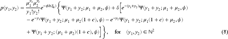
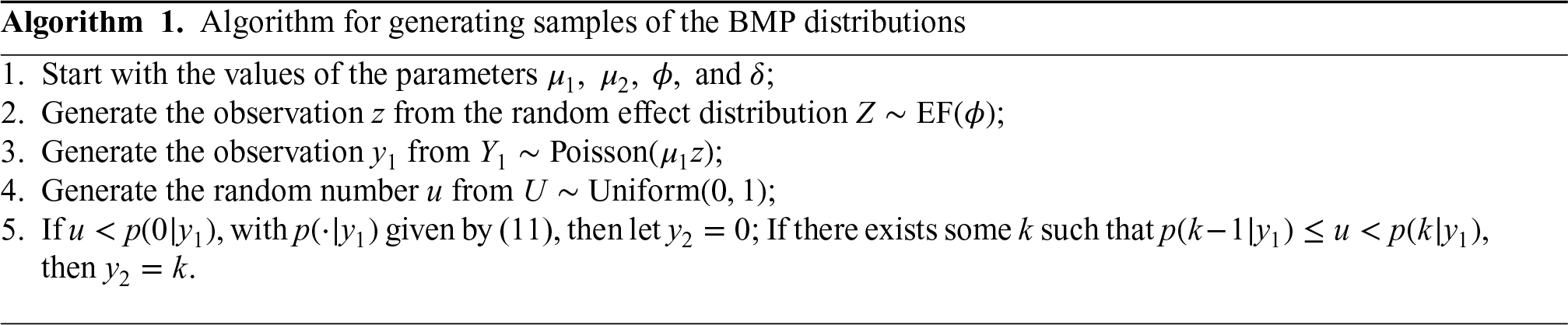
We obtain an explicit form for the joint probability function of the BMP distributions in the next proposition. In particular, this expression will enable us to perform the maximum likelihood estimation of parameters.
Let

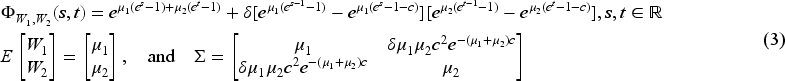
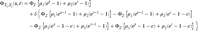
Next, we provide the moment generating function, a useful tool to explicit the moment structure of the proposed BMP distributions.
The moment generating function of the BMP distributions, say
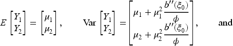
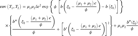
The covariance between
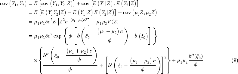
Through moment structure, we notice that the BMP distribution is overdispersed. In fact, for any positive random variable
A small correlation coefficient study between our BMP and BP models is provided in Section 1 of the Supplemental Material.
The conditional BP distribution is straightforward to obtain, as provided by Cui and Zhu.
26
Hence, in what follows, we present its probability mass function and moment generating function since we will use these attributes to derive some results needed to generate samples from our proposed class of BMP distributions. Thus, the probability mass function of the conditional BP distribution is given by the following equation:

The distribution of
In Table 1, we present some quantities associated with two models belonging to the BMP class, the BNB and BP-inverse Gaussian (BPIG) distributions, which arise when the random effect
Quantities associated with gamma and the inverse-Gaussian heterogeneity
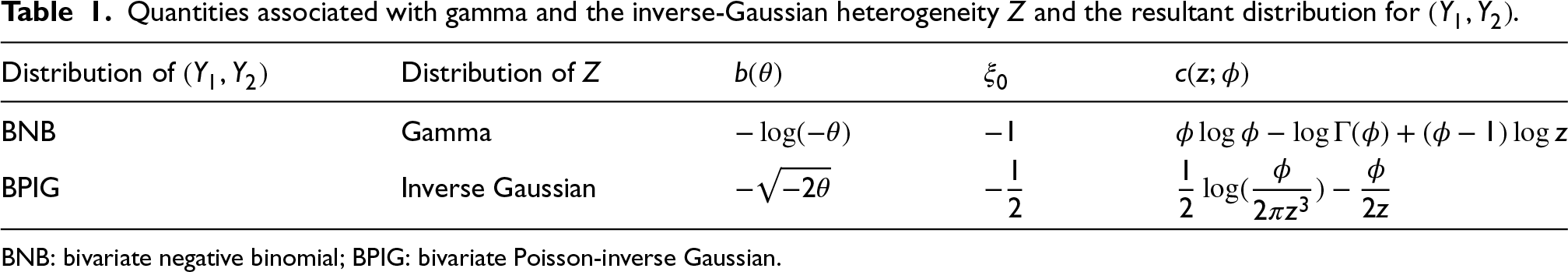
BNB: bivariate negative binomial; BPIG: bivariate Poisson-inverse Gaussian.
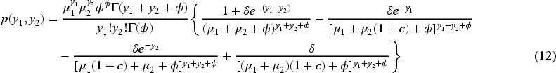
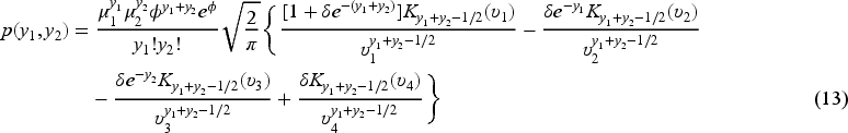
By using equation (8) from Proposition 2.3 and the quantities provided in Table 1, we obtain explicit forms for the joint pmf of the BNB (equation (12)) and the BPIG (equation (13)) distributions, which are, respectively, given by the following equations:

In the next section, we introduce the class of BMP regression models and discuss how to perform inference, including Monte Carlo simulation results for checking the finite-sample behavior of the proposed estimators and related standard error evaluation.
In this section, we discuss the maximum likelihood method for inference of the parameters of the BMP regression models. For bivariate count random variables 

Considering 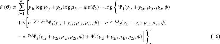
A Monte Carlo study is performed to evaluate the performance of MLEs for finite samples. For this simulation analysis, we have set, in expressions (14) and (15), 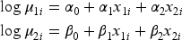
We start the analysis of the simulation results from Table 2, which comprises the empirical mean and the root mean square error (RMSE) of the parameter estimates for the BNB regression model. We observe small bias and RMSE across most sample size configurations, except for sample sizes 50 and 100. Notably, the parameters
Empirical mean and root mean square error (in parentheses) of the estimates for the BNB regression model, with
.
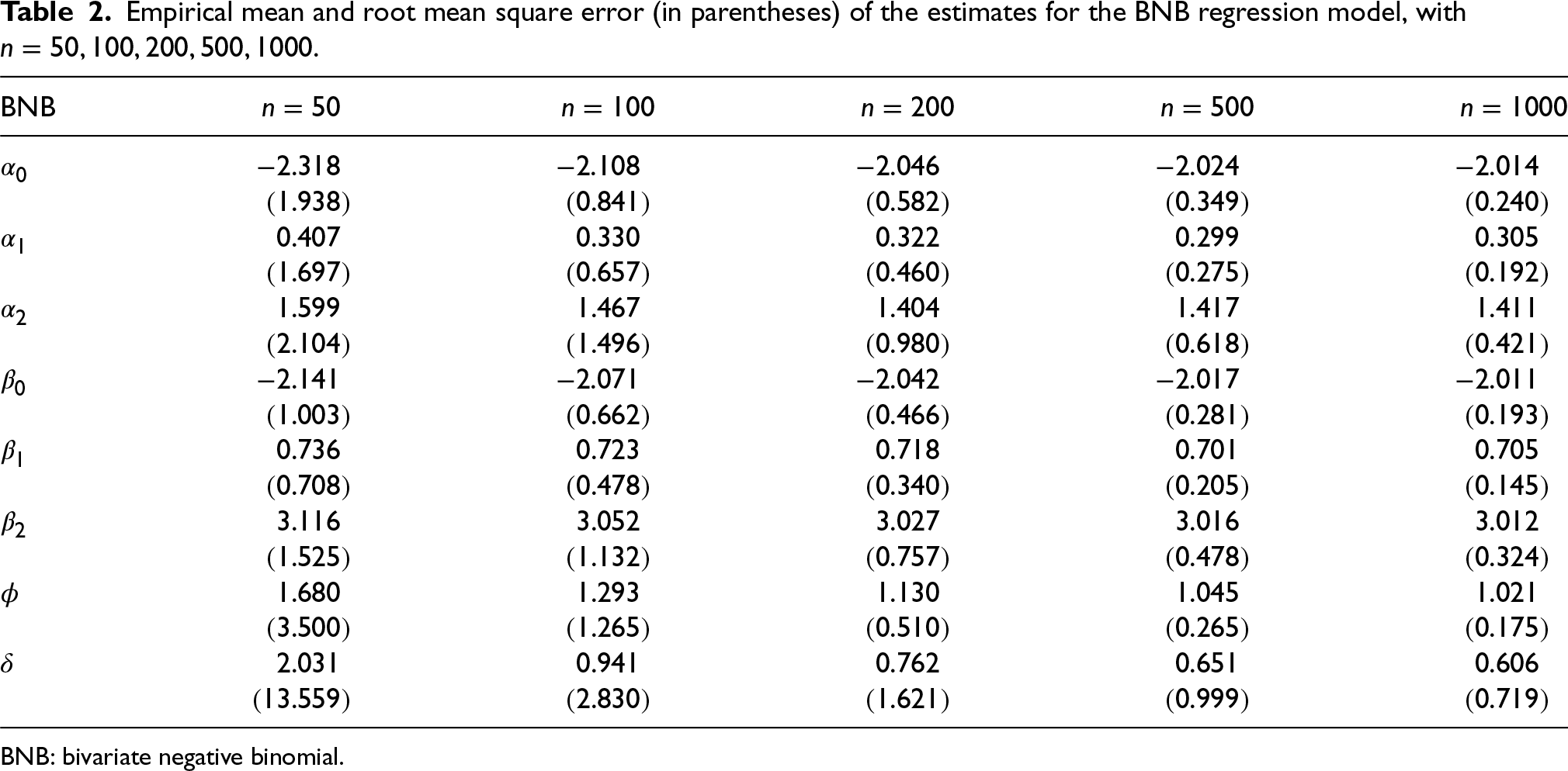
Empirical mean and root mean square error (in parentheses) of the estimates for the BNB regression model, with
BNB: bivariate negative binomial.
The suitable performance of the estimation method based on the simulation study is reported in Figures 3 and 5 in the Supplemental Material, which covers the histograms of the standardized (mean-standard deviation) parameter estimates, seeming to be asymptotically normally distributed with the increase of the sample size, as they follow along with normal density curves.
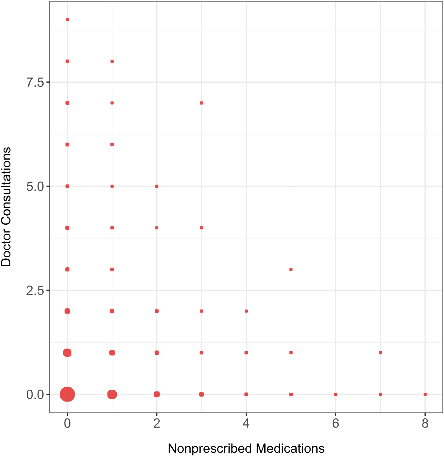
Descriptive data analysis on the number of doctor consultations versus the number of non-prescribed medications, from a sample of the Australian Health Survey (AHS) study, 1977–1978.
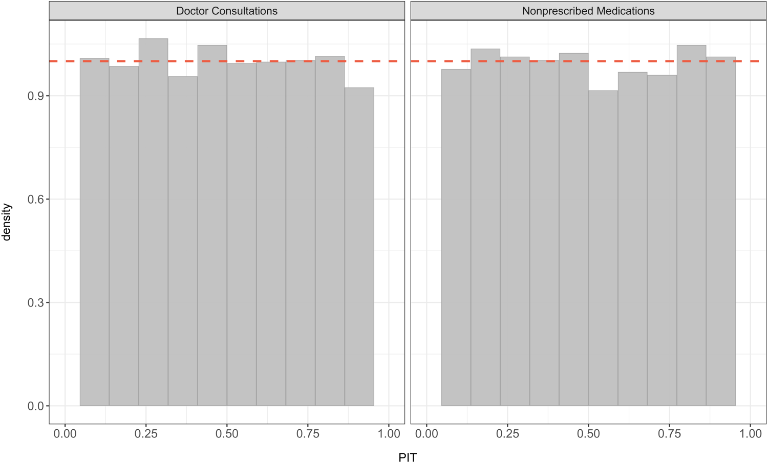
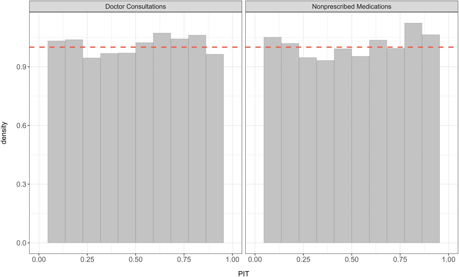
Histograms of the randomized PIT under the BNB regression for the number of doctor consultations and the number of non-prescribed medications. PIT: probability integral transform; BNB: bivariate negative binomial.
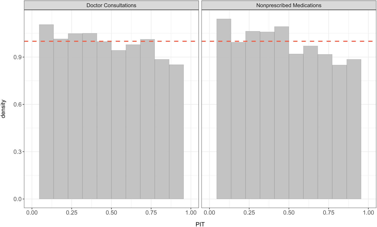
Histograms of the randomized PIT under the BPIG regression for the number of doctor consultations and the number of non-prescribed medications. PIT: probability integral transform; BPIG: bivariate Poisson-inverse Gaussian.
Analyzing the simulation study for the BPIG regression model, through Table 3, we anticipate results similar to that of the BNB regression model. Therefore, small bias and RMSE for almost all configurations of considered sample sizes and asymptotic normal distribution of the parameter estimates, as the sample size increases, except the scenarios with sample sizes 50 and 100. The histograms of the standardized parameter estimates, along with a normal density curve, have a pattern similar to those produced by the BNB regression model, as presented in Figures 4 and 6 from the Supplemental Material.
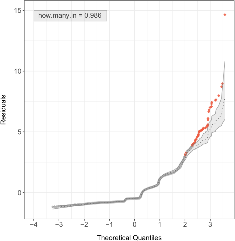
Simulated envelopes for Pearson residuals under the bivariate negative binomial (BNB) regression model for the number of doctor consultations and the number of non-prescribed medications.
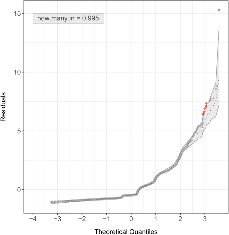
Simulated envelopes for Pearson residuals under the bivariate Poisson-inverse Gaussian (BPIG) regression model for the number of doctor consultations and the number of non-prescribed medications.
Histograms of the randomized PIT under the BP regression for the number of doctor consultations and the number of non-prescribed medications. PIT: probability integral transform; BP: bivariate Poisson.
Empirical mean and root mean square error (in parentheses) of the estimates for the BPIG regression model, with
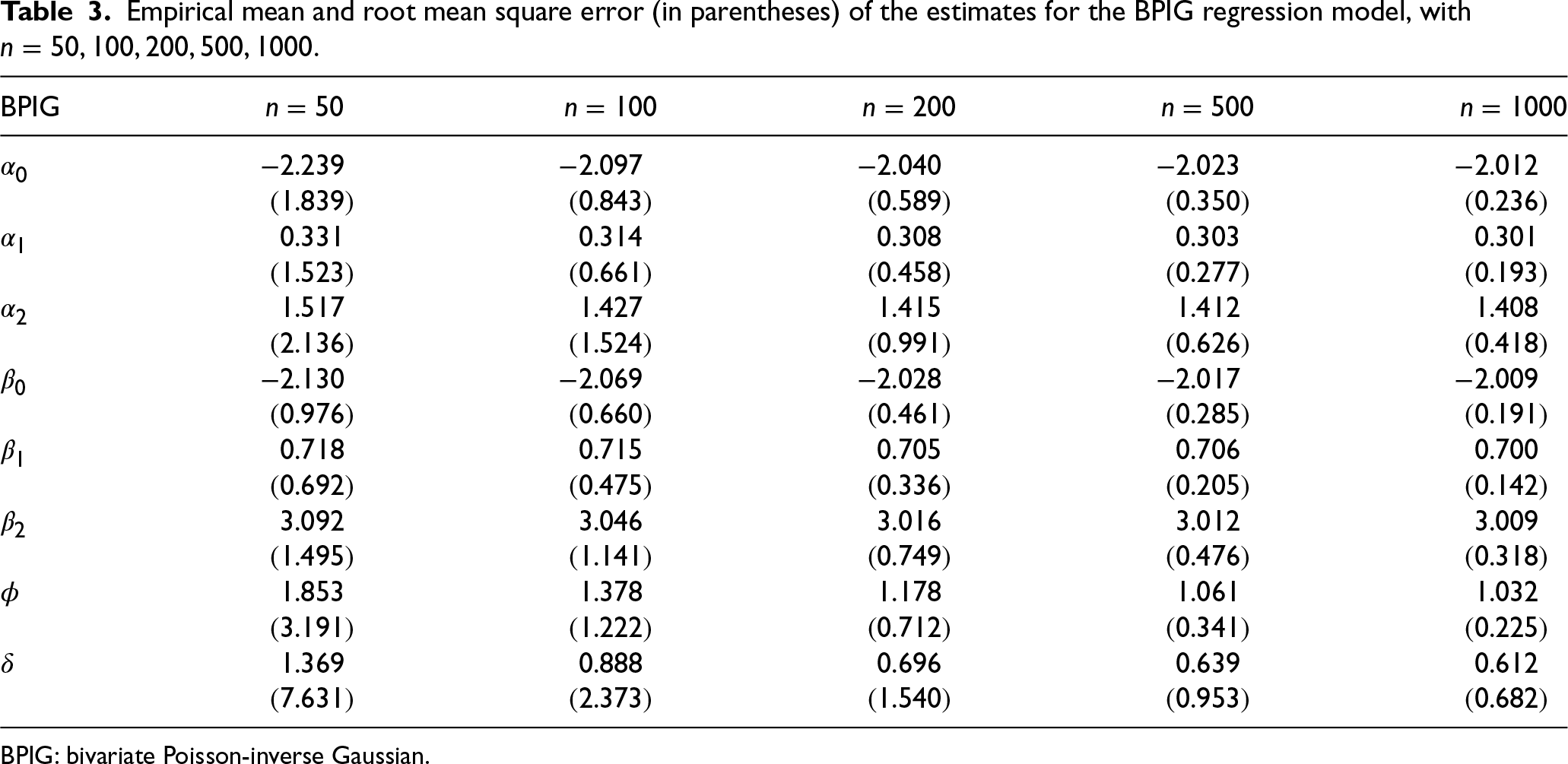
BPIG: bivariate Poisson-inverse Gaussian.
We now present in Tables 4 and 5 the empirical standard error of the estimates stated in the Monte Carlo simulation and the average of the standard errors of these estimates obtained via the Hessian matrix. From the results of these tables, we conclude that the outcomes of the Hessian matrix are consistent for estimating the standard errors of the parameter estimates, for both the BNB and the BPIG regression models, except for sample size 50.
Empirical and Hessian derived standard errors of the parameter estimates for the BNB regression model, with
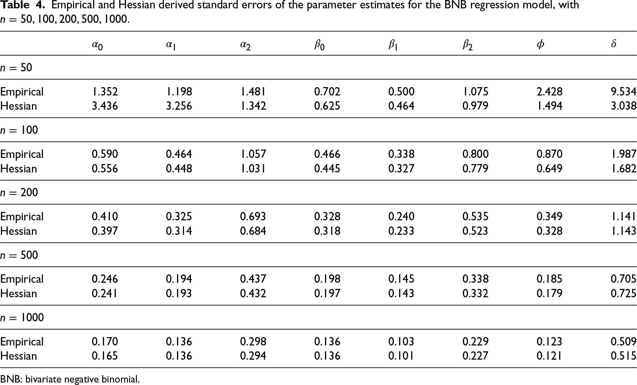
BNB: bivariate negative binomial.
Empirical and Hessian derived standard errors of the parameter estimates for the BPIG regression model, with
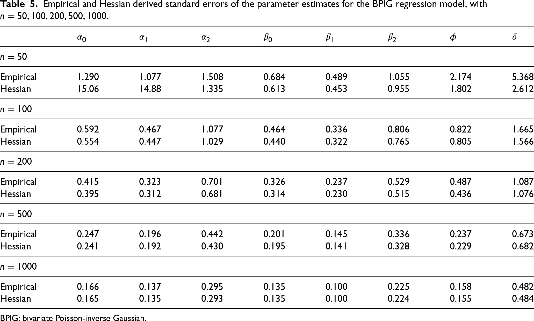
BPIG: bivariate Poisson-inverse Gaussian.
More simulated results are provided in the Supplemental Material (Section 2) about the adverse effects of incorrectly ignoring conditional dependence, that is assuming
The model specification encompasses the following stages: estimation, diagnostic checking, and inference. This section discusses some techniques for performing such tasks. In particular, we are interested in investigating possible sources of correlation. To this end, we conduct hypothesis testing involving the correlation parameter
LRT and simulated results
Regarding some hypotheses on the BMP regression models, we are interested in determining when the parameter 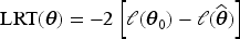
Empirical type-I errors of the LRT under the BNB regression model, with
.
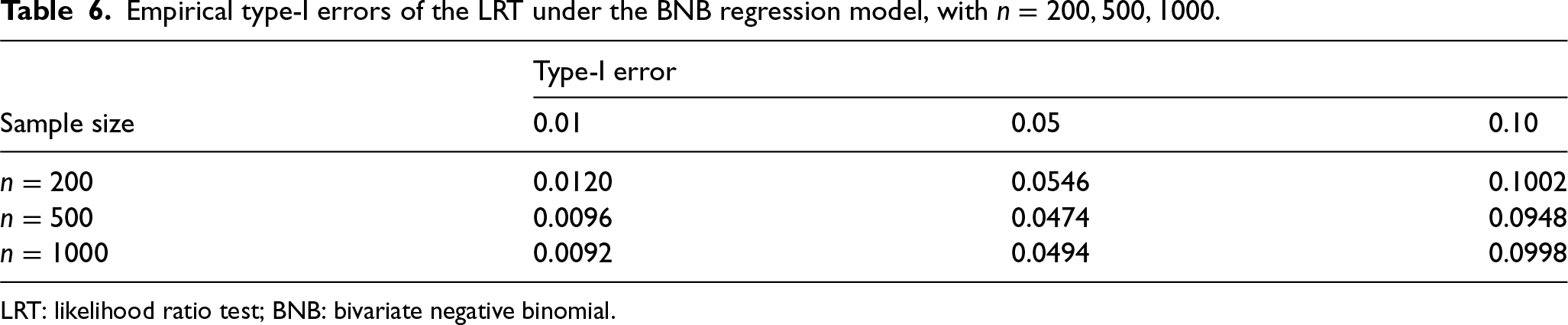
Empirical type-I errors of the LRT under the BNB regression model, with
LRT: likelihood ratio test; BNB: bivariate negative binomial.
Empirical type-I errors of the LRT under the BPIG regression model, with
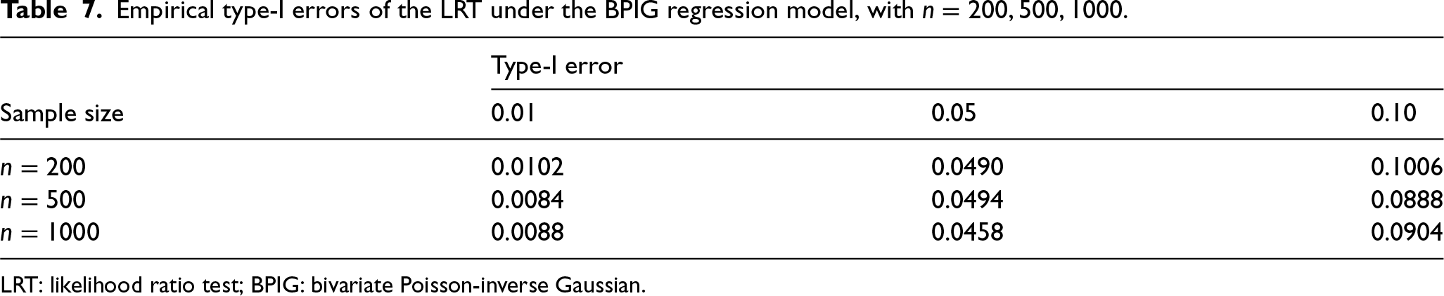
LRT: likelihood ratio test; BPIG: bivariate Poisson-inverse Gaussian.
Considering the model evaluation stage, one might conduct residual analysis and use goodness-of-fit measures. According to Cameron and Trivedi,
7
one carries the residual analysis for many purposes, such as to detect model misspecification, outliers, poor fit, and influential observations. Therefore, techniques to perform residual analysis will measure the departure between the fitted and the original values of the dependent variable, indicating that it is essential. In addition, a visual inspection may potentially indicate the nature of model misspecification and the magnitude of its effect. The literature has proposed miscellaneous residuals for count data, and one of the nominees presented by Cameron and Trivedi
7
is the Pearson residual, also known as the standardized residual. In order to check the goodness-of-fit of the joint model instead of a marginal approach, we consider the Pearson residual of the sum of the count variables as follows:
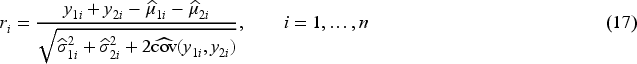
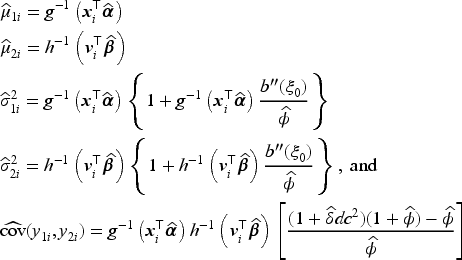
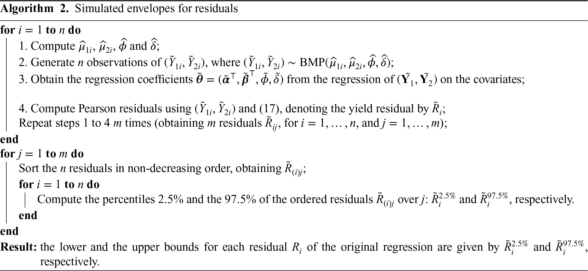
An ordinary way to employ residuals is to plot them against the normal quantiles. However, even though Pearson’s residuals have zero mean and unit variance for large samples, they are skewed in distribution. Therefore, we expect the normal approximation to be poor, even for moderate sample sizes. A path to overpower this barrier is to construct simulated envelopes for the residuals, as suggested by Atkinson, 29 and Hinde and Demétrio. 30 The steps to produce simulated envelopes for count regression models follow the description of Algorithm 2. Here, we will demonstrate the performance of these simulated envelopes in the empirical illustration in Section 5.
Regarding the calibration and sharpness of the model, Czado et al. 31 pointed out that a calibrated model refers to the consistency between the observed variable and its predictions. Hence, one can request the probability integral transform (PIT)32,33 to check if it is possible to conclude that the observations of a continuous variable are derived from the suggested predictive distribution. For this, we can proceed graphically or through hypothesis tests since, for suitable cases, the PIT must be uniform in distribution.
However, when it comes to a discrete variable, it is well-known that the PIT does not have a uniform distribution. Consequently, the literature introduced the randomized PIT,34–36 which follows the standard uniform distribution, to make it available for count data. Therefore, we suggest using the randomized probability integral transform histogram for calibration model control as a diagnostic tool:

Residual analysis and diagnostics were conducted marginally to smooth the model evaluation process. The bivariate residual analysis is not straightforward since the idea of sample ordering is lost, as pointed out by Moral et al. 37 Moreover, regarding model calibration, it is not trivial to determine if the observations can be said to be derived from the suggested predictive distribution, not to mention that the bivariate PIT is no longer uniformly distributed. For a thorough assessment of the model, which will be further developed in future research for the class of BMP regression models, we refer to the paper by Genest and Rivest, 38 which proposes a bivariate probability integral transformation based on copulas and makes considerations for a multivariate extension. Also, we refer to the work by Moral et al., 37 in which the authors propose a generalization of the simulated envelopes yielding simulated polygons for bivariate residual analysis. We illustrate the usefulness of the proposed forthright residual analysis and randomized probability integral transformation in the real data analysis in Section 5.
The proposed class of models was motivated by the problem of finding the association between the number of consultations with a doctor and consumption of non-prescription medication. The dataset regards information on health conditions and, as well, demographic and socioeconomic characteristics of the individuals, collected from the 1977–1978 AHS, conducted by the Australian Bureau of Statistics (ABS). Since 1989, the Australian health survey series has been part of the National Health Survey (NHS), with similar information, and one can grasp more about the NHS at https://www.abs.gov.au/statistics/health.
The employed dataset, a sample of the 1977–1978 AHS, was first analyzed by Cameron et al.
39
through a microeconometric model for healthcare demand. This dataset is available in the book by Cameron and Trivedi
7
and, later, in the book by Faraway,
40
which made it ready for use on the faraway package in the CRAN of
To investigate the association between the count of doctor consultations and the non-prescribed drug intake, we apply the proposed model on the sample of the 1977–1978 AHS which contains attributes of 5190 individuals aged 15 years or older. Unlike previous research, we considered, as count responses, variables that are negatively correlated—the number of consultations with a doctor and the number of non-prescribed medications. The explanatory variables in this dataset are enumerated as follows
Regarding covariates, there is more than one type of health insurance, such as private and government coverage, and, as well, there is more than one combination of the
Figure 1 shows the number of non-prescribed medications versus the number of consultations with a doctor, with the size of the points in this plot being proportional to the frequency of these paired count variables. In a first look at the plot, we notice small counts for both variables, with a higher proportion of zero doctor consultations and, as well, zero non-prescribed medications. Also, as anticipated, a lower number of non-prescribed medications would be expected for an individual with a higher count of consultations with a doctor, as this patient will be more likely to purchase prescribed medications. Conversely, a higher number of non-prescribed medications is associated with fewer doctor appointments. Again, this was expected since these individuals, without medical advice, will acquire non-prescribed medications. Thus, it seems that for this dataset, as we can see through Figure 1, an inverse relationship between the number of non-prescribed medications and the number of consultations with a doctor, indicating the existence of a negative correlation.
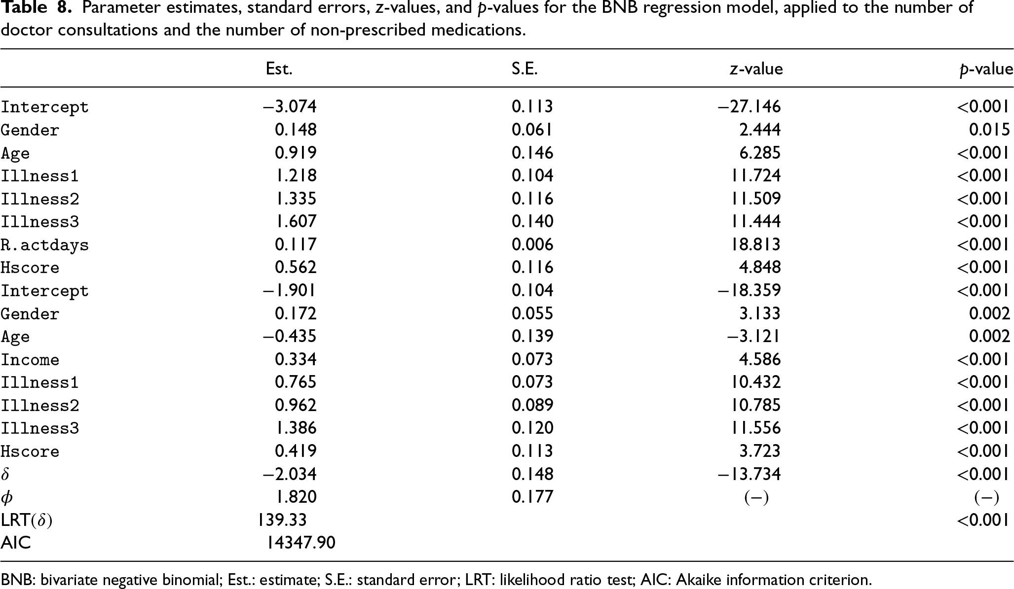
To fit statistical models, we consider the BNB and the BPIG regressions, which belong to our class of BMP models. The results of the BNB regression model are reported in Table 8 which presents the parameter estimates, the standard error estimates, z-values, and associated p-values. After initial data analysis, the model fit chose as significant covariates
With respect to the BPIG regression model, the preliminary analysis selected the same covariates as in the fit of the BNB regression model, with the addition of the explanatory variable
Parameter estimates, standard errors, z-values, and p-values for the BNB regression model, applied to the number of doctor consultations and the number of non-prescribed medications.
Parameter estimates, standard errors, z-values, and p-values for the BNB regression model, applied to the number of doctor consultations and the number of non-prescribed medications.
BNB: bivariate negative binomial; Est.: estimate; S.E.: standard error; LRT: likelihood ratio test; AIC: Akaike information criterion.
Parameter estimates, standard errors, z-values, and p-values for the BPIG regression model, applied to the number of doctor consultations and the number of non-prescribed medications.
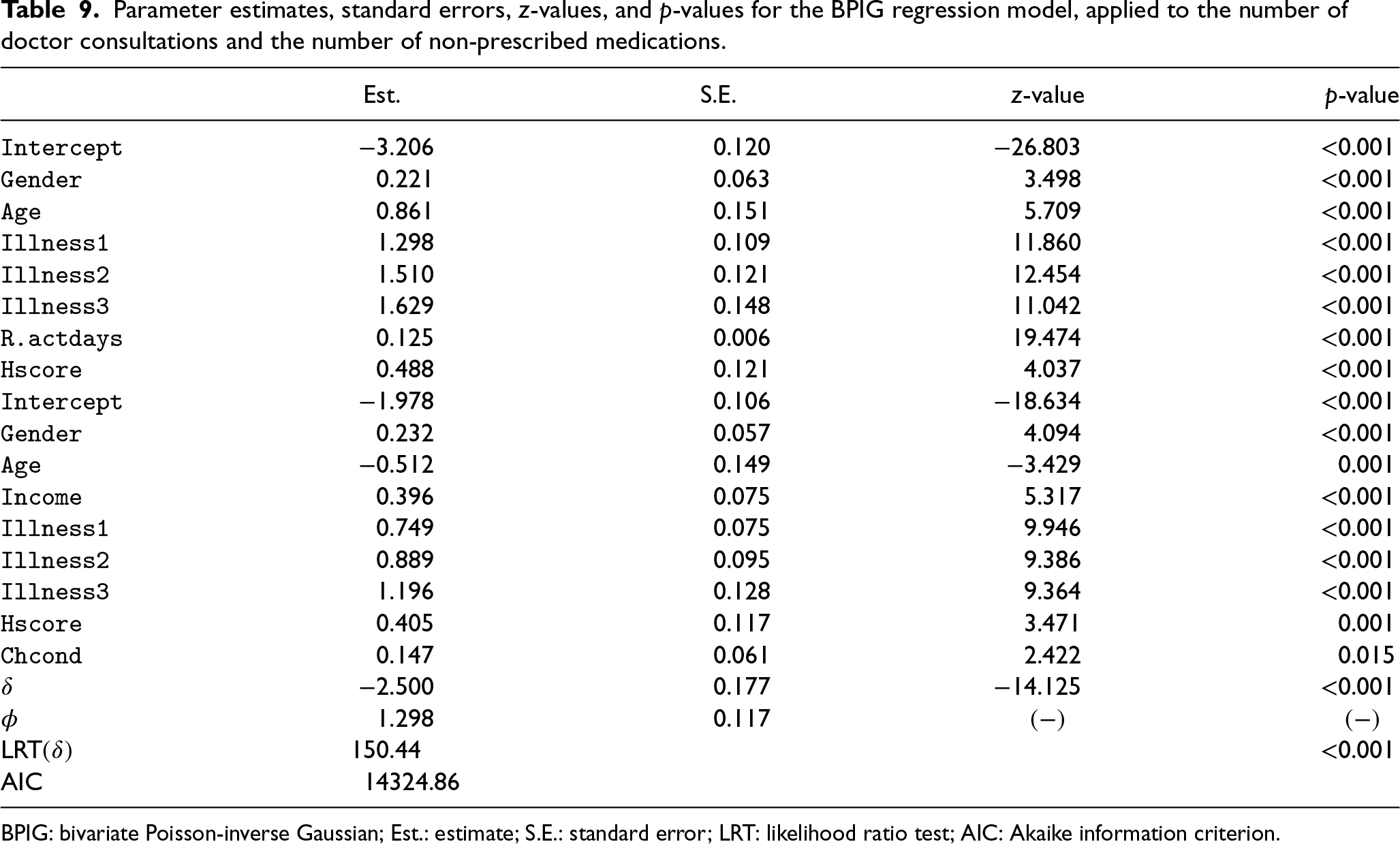
BPIG: bivariate Poisson-inverse Gaussian; Est.: estimate; S.E.: standard error; LRT: likelihood ratio test; AIC: Akaike information criterion.
To check potential flaws in the model and prediction, we first examined the BNB regression model. The randomized PIT histogram in Figure 2 appears to be approximately uniformly distributed, inducing a consistency for both responses, the number of consultations with a doctor, and the number of non-prescribed medications. Likewise, the BPIG regression model also suggests a consistency for the number of doctor consultations and the number of non-prescribed medications, as we observe calibration in Figure 3 through the histograms that appear to be nearly uniformly distributed.
Continuing the modeling cycle, we are now interested in verifying whether the assumed BMP distribution is adequate for the dataset considered here. Figures 4 and 5 deliver the simulated envelopes for the Pearson residual against the theoretical quantiles of the standard normal distribution, respectively, for the BNB and the BPIG regression models. Assuming the unobserved heterogeneity is either gamma-distributed or inverse-Gaussian distributed, both choices look suitable since almost all residuals remain within the simulated envelopes.
Note that around 98.6% of the residuals within the simulated envelopes for the BNB regression model, and almost 99.5% for the BPIG regression model, with even better performance for the latter.
Not considering overdispersion in the modeling process can compromise the data analysis. Thus, the BP regression model was applied to underline the need for a model that allows overdispersion; the summary fit is provided in Table 10. Regarding its randomized PIT, Figure 6 exposes a slight deviation from uniformity, implying a reduced calibration compared to the BMP regression models. Even more worrisome, Figure 7 points out that the BP distribution is not indicated for this dataset since only 56.1% of the residuals lie inside the simulated envelopes.
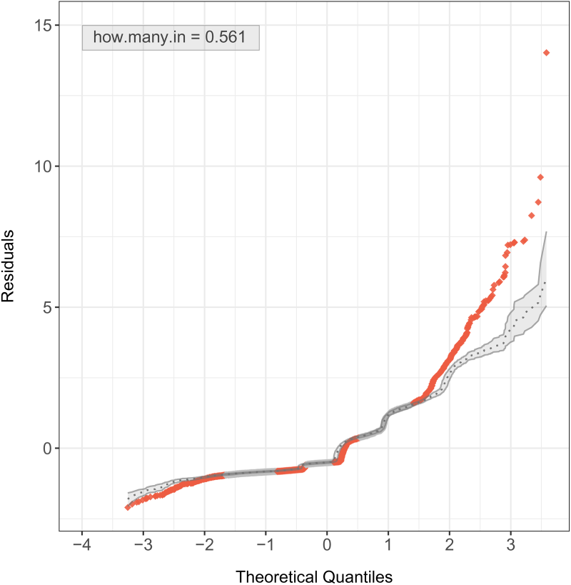
Simulated envelopes for Pearson residuals under the bivariate Poisson (BP) regression model for the number of doctor consultations and the number of non-prescribed medications.
Parameter estimates, standard errors, z-values, and p-values for the BP regression model, applied to the number of doctor consultations and the number of non-prescribed medications.
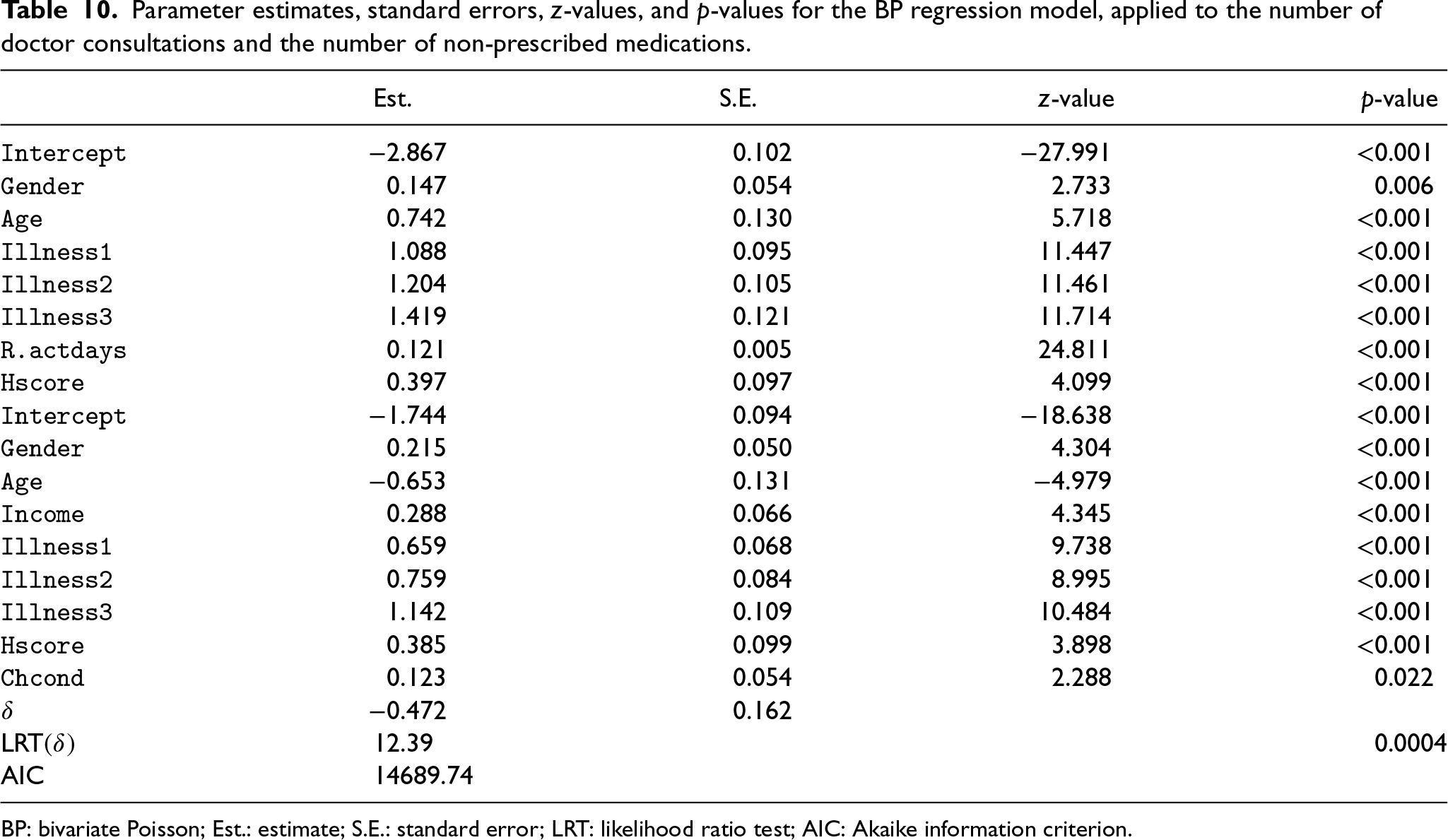
BP: bivariate Poisson; Est.: estimate; S.E.: standard error; LRT: likelihood ratio test; AIC: Akaike information criterion.
We conclude this section on the interpretation of the model, using the relativities provided in Table 11. These measures aim to compare a covariate’s category with its baseline in terms of predicted response.
Relativities of the explanatory variables, to estimate the number of doctor consultations and non-prescribed medications, under the BPIG regression model.
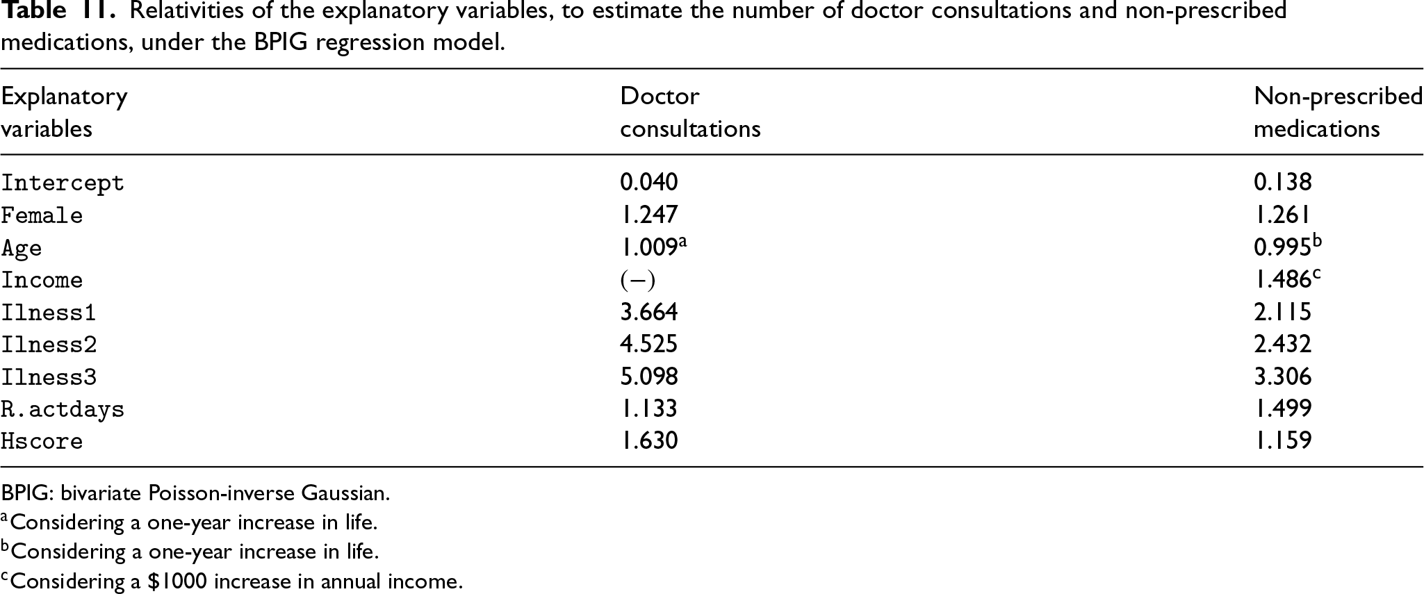
BPIG: bivariate Poisson-inverse Gaussian.
To proceed with the interpretation of the model, we chose the BPIG regression as the final model for this empirical illustration since it presents the best performance due to the conjuncture of its results. Table 11 reveals that the expected number of doctor consultations and non-prescribed medications is about 25% and 26%, respectively, higher for
We have introduced a new class of regression models to analyze bivariate count data. We have considered a latent component, with distribution belonging to the exponential family, to account for the unobserved heterogeneity inherent to such data. We proposed the maximum likelihood method for inference on the model parameters. We have evaluated the MLEs for two particular cases of our class, the BNB, and the BPIG models, concluding with a good finite-sample performance of the proposed estimators in both models. We also provided a general measure of model calibration and simulated envelopes for checking the model adequacy of our BMP regression models.
A complete statistical analysis of a random sample dataset of the 1977–1978 AHS from the Australian Bureau of Statistics has been conducted. We studied the number of doctor consultations by individuals and the number of non-prescribed medications acquired by these individuals, using these variables for joint modeling through the proposed BMP models. The bivariate analysis of this AHS count dataset is, to the best of our knowledge, a new contribution once we deliver a complete analysis of the data, showing that the BMP models provide an adequate joint fit to the number of doctor consultations and non-prescribed medications. We also illustrated that ignoring the unobserved heterogeneity in such data can lead to a poor model fit.
Towards future research, noteworthy issues that deserve further investigation are (i) the generalization of the model allowing for a varying dispersion parameter and a regression framework for the
Supplemental Material
sj-zip-1-smm-10.1177_09622802251345332 - Supplemental material for Paired count regressions for modeling the number of doctor consultations and non-prescribed drugs intake
Supplemental material, sj-zip-1-smm-10.1177_09622802251345332 for Paired count regressions for modeling the number of doctor consultations and non-prescribed drugs intake by Jussiane Nader Gonçalves,Wagner Barreto-Souza and Hernando Ombao in Medical Research
Supplemental Material
sj-pdf-2-smm-10.1177_09622802251345332 - Supplemental material for Paired count regressions for modeling the number of doctor consultations and non-prescribed drugs intake
Supplemental material, sj-pdf-2-smm-10.1177_09622802251345332 for Paired count regressions for modeling the number of doctor consultations and non-prescribed drugs intake by Jussiane Nader Gonçalves,Wagner Barreto-Souza and Hernando Ombao in Medical Research
Footnotes
Acknowledgements
We express our gratitude to two anonymous Referees for their valuable comments and suggestions.
Declaration of conflicting interests
The author(s) declared no potential conflicts of interest with respect to the research, authorship, and/or publication of this article.
Funding
The author(s) disclosed receipt of the following financial support for the research, authorship, and/or publication of this article.
Supplemental material
Supplemental material for this article is available online. This article includes supplemental material with additional numerical results. We also provide the R code and real data used in our empirical illustration to ensure the results are reproducible.
Notes
Appendix
[Proposition 2.3]
For The integrals involved in (19) can be obtained by using the fact that
[Proposition 2.4]
By using properties of the conditional mean, variance, and covariance, and the two first cumulants of the BS distribution, we have that
References
Supplementary Material
Please find the following supplemental material available below.
For Open Access articles published under a Creative Commons License, all supplemental material carries the same license as the article it is associated with.
For non-Open Access articles published, all supplemental material carries a non-exclusive license, and permission requests for re-use of supplemental material or any part of supplemental material shall be sent directly to the copyright owner as specified in the copyright notice associated with the article.