Fitting exponential regression models with two-way fixed effects

Abstract

In this article, we introduce the commands twexp and twgravity, which implement the estimators developed in Jochmans (2017, Review of Economics and Statistics 99: 478–485) for exponential regression models with two-way fixed effects. twexp is applicable to generic n × m panel data. twgravity is written for the special case where the dataset is a cross-section on dyadic interactions between n agents. A prime example is cross-sectional bilateral trade data, where the model of interest is a gravity equation with importer and exporter effects. Both twexp and twgravity can deal with data where n and m are large, that is, where there are many fixed effects. These commands use Mata and are fast to execute.

1 Introduction

The exponential regression model finds wide application in the analysis of nonnegative outcomes such as count data. This model has also shown itself to be an attractive alternative to the log-linearized regression model. Indeed, following Santos Silva and Tenreyro (2006), constant-elasticity models are now routinely fit from data in levels rather than logarithms. In this article, we present two new commands to estimate exponential regressions with two-way fixed effects.

We consider double-indexed data on a nonnegative outcome, y_ij , and a p-vector of regressors, x _ij . The command twexp is designed to estimate the slope vector γ in the n × m panel mode

$y_{ij}=e({\alpha }_i+{\beta }_j+x_{ij}^{\top }\gamma ){\epsilon }_{ij}\hspace{0.17em}\hspace{0.17em}\hspace{0.17em}\hspace{0.17em}\hspace{0.17em}E({\epsilon }_{ij}|x_{11},. . . ,x_{nm}) =\hspace{0.17em}\hspace{0.17em}1$

1

where i = 1,…, n and j = 1,…, m, and we let e(a) := exp(a). Here α_i and β_j are fixed effects, and ε_ij is a latent disturbance. A slight variation to this is a cross-sectional dataset in which we observe outcomes and regressors for the n × (n − 1) pairwise interactions between agent i = 1,…, n and j ≠ i. This is different from the panel-data case because here we do not observe y_ii and x _ii . The command twgravity is designed to handle this case. Its name is derived from the leading example of such an application being the estimation of a gravity equation from a cross-section of bilateral trade flows. Here the outcome is the directed trade flow from i to j, the regressors are measures of distance or (dis)similarity between i and j, and α_i and β_j are exporter and importer effects, respectively.

The most popular estimator of (2) is the pseudo-maximum-likelihood estimator (PMLE) that arises from treating the y_ij as conditionally independent Poisson variates. If we introduce the shorthand

$u_{ij}({\alpha }_i, {\beta }_j,\gamma ) :=y_{ij}-e({\alpha }_i+{\beta }_j+x_{ij}^{\top }\gamma )$

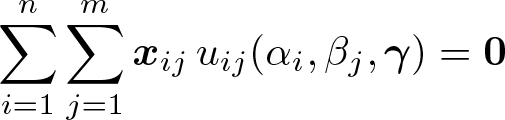
the PMLE solves the p first-order conditions for γ ,

${\displaystyle \sum _{i-1}^n{\displaystyle \sum _{j=1}^m{x}_{ij}{u}_{ij}\left({\alpha }_i,\hspace{0.17em}{\beta }_j,\hspace{0.17em}\gamma \right)}}=0$

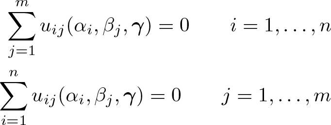
jointly with the n + m first-order conditions for the effects α ₁,…, α_n and β ₁,…, β_m ,

$\begin{array}{l}{\displaystyle \sum _{j=1}^m{u}_{ij}\left({\alpha }_i,\hspace{0.17em}{\beta }_j,\hspace{0.17em}\gamma \right)}=0\hspace{0.17em}\hspace{0.17em}\hspace{0.17em}\hspace{0.17em}\hspace{0.17em}\hspace{0.17em}\hspace{0.17em}\hspace{0.17em}\hspace{0.17em}\hspace{0.17em}i=1,\hspace{0.17em}.\hspace{0.17em}.\hspace{0.17em}.\hspace{0.17em},\hspace{0.17em}n\\ {\displaystyle \sum _{i=1}^n{u}_{ij}\left({\alpha }_i,\hspace{0.17em}{\beta }_j,\hspace{0.17em}\gamma \right)}=0\hspace{0.17em}\hspace{0.17em}\hspace{0.17em}\hspace{0.17em}\hspace{0.17em}\hspace{0.17em}\hspace{0.17em}\hspace{0.17em}\hspace{0.17em}\hspace{0.17em}i=1,\hspace{0.17em}.\hspace{0.17em}.\hspace{0.17em}.\hspace{0.17em},\hspace{0.17em}m\end{array}$

Subject to a suitable normalization on the fixed effects, such as ${\sum }_{i=1}^n{\alpha }_i= {\sum }_{j=1}^m{\beta }_j$ . Despite the presence of the growing number of nuisance parameters, the estimator of γ is consistent and has a correctly centered limit distribution either when n is large and m is small or when both n and m are large (and of a similar magnitude). Details on the theoretical properties are available in Wooldridge (1999) and Fernández-Val and Weidner (2016).

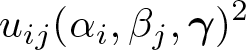
The pseudo-Poisson approach suffers from two drawbacks. The first is numerical. Indeed, the large number of fixed effects implies that a simple approach that combines, say, poisson with n + m dummy variables will be infeasible in many datasets. The commands poi2hdfe (Guimarães 2016) and ppmlhdfe (Correia, Guimarães, and Zylkin 2019) are designed especially to deal with this problem and are useful alternatives here. The second drawback is that the plug-in estimator of the covariance matrix of the above moment conditions is severely biased. The origin of the problem is again the estimation of the incidental parameters. Indeed, calculating the covariance matrix requires estimating terms involving

$u_{ij}{\left({\alpha }_i, {\beta }_j,\gamma \right)}^2$

which requires estimates of the fixed effects. These are both numerous and estimated with low precision, creating an incidental parameter bias in the estimated covariance matrix. The bias can be severe, as evidenced by the simulation results in Egger and Staub (2016), Jochmans (2017), and Pfaffermayr (2019). The practical implication of this is that the standard errors will usually not be an accurate reflection of the statistical precision of the parameter estimates. Often, they will be too small. Consequently, the reported confidence interval will be too narrow, and test procedures will overreject under the null.

Equation (2) is an important member of the class of multiplicative error models. For such models, moment conditions have been derived that are free of fixed effects (Charbonneau 2013; Jochmans 2017). They allow inference on γ to be separated from estimation of α ₁,…, α_n and β ₁,…, β_m . twexp and twgravity implement estimators based on these moments. Both commands are designed to be computationally efficient and are fast to implement. Hence, our commands should be a useful addition to the toolbox of empirical researchers working with count data and trade data. Furthermore, because the whole problem is free of nuisance parameters, the standard errors do not suffer from an incidental parameter bias.

2 Moment conditions and estimators

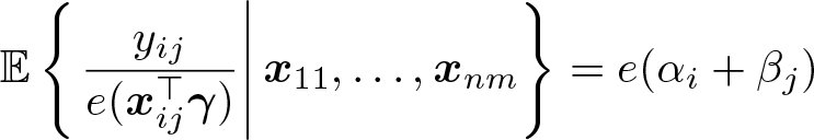
Consider (2) under the assumption that the errors are (conditionally) mutually independent. Then, using

$\mathbb{\text{E}}\hspace{0.17em}\left\{\frac{y_{ij}}{e\left(x_{ij}^{\top }\gamma \right)}\hspace{0.17em}|\hspace{0.17em}{x}_{11},\hspace{0.17em}.\hspace{0.17em}.\hspace{0.17em}.\hspace{0.17em},x_{nm}\right\}=e\left({\alpha }_i+{\beta }_j\right)$

for all (i, j), we have

$\mathbb{\text{E}}\hspace{0.17em}\left\{\frac{y_{ij}}{e\left(x_{ij}^{\top }\gamma \right)}\frac{y_{i\text{'}j\text{'}}}{e\left(x_{i\text{'}j\text{'}}^{\top }\gamma \right)}-\frac{y_{ij\text{'}}}{e\left(x_{ij\text{'}}^{\top }\gamma \right)}\frac{y_{i\text{'}j}}{e\left(x_{i\text{'}j}^{\top }\gamma \right)}\hspace{0.17em}|\hspace{0.17em}{x}_{11},\hspace{0.17em}.\hspace{0.17em}.\hspace{0.17em}.\hspace{0.17em},x_{nm}\right\}=0$

2

for all i, i^′ and j, j^′ . This (conditional) moment condition for γ is free of incidental parameters. Equation (2) implies unconditional moment conditions that can form the basis of a method of moment estimator of γ . Our commands implement two of these estimators.

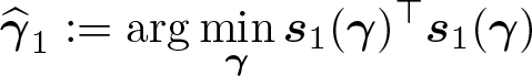
The first estimator, which we dub generalized method of moments (GMM1) below, uses the levels of the covariates, x _ij , as instruments. It is the solution to

$s_1\left(\gamma \right):={\displaystyle \sum _{i=1}^n{\displaystyle \sum _{i\text{'}=1}^n{\displaystyle \sum _{j=1}^m{\displaystyle \sum _{j\text{'}=1}^m{x}_{ij}}\left\{\frac{y_{ij}}{e\left(x_{ij}^{\top }\gamma \right)}\frac{y_{i\text{'}j\text{'}}}{e\left(x_{i\text{'}j\text{'}}^{\top }\gamma \right)}-\frac{y_{ij\text{'}}}{e\left(x_{ij\text{'}}^{\top }\gamma \right)}\frac{y_{i\text{'}j}}{e\left(x_{i\text{'}j}\gamma \right)}\right\}}=0}}$

This is a system of p equations and is therefore just identified. ¹ Consequently, the estimator is

${\widehat{\gamma }}_1\hspace{0.17em}:=\arg \hspace{0.17em}\min \hspace{0.17em}{s}_1{\left(\gamma \right)}^{\top }{s}_1\left(\gamma \right)$

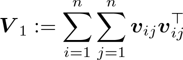
Under suitable regularity conditions, ${\widehat{\gamma }}_1$ is consistent and asymptotically normal. Its asymptotic variance has a sandwich form and can be estimated as $Q_1^{-1}{V}_1{Q}_1^{-\top }$ , where

$Q_1\hspace{0.17em}:=-{\displaystyle \sum _{i=1}^n{\displaystyle \sum _{i\text{'}=1}^n{\displaystyle \sum _{j=1}^m{\displaystyle \sum _{j\text{'}=1}^m{x}_{ij}}\left\{\frac{y_{ij}{y}_{i\text{'}j\text{'}}{\left(x_{ij}+x_{i\text{'}j\text{'}}\right)}^{\top }}{e\left(x_{ij}^{\top }\widehat{{\gamma }_1}\right)e\left(x_{i\text{'}j\text{'}}^{\top }\widehat{{\gamma }_1}\right)}-\frac{y_{ij}{y}_{i\text{'}j}{\left(x_{i\text{'}j}+x_{ij\text{'}}\right)}^{\top }}{e\left(x_{ij\text{'}}^{\top }\widehat{{\gamma }_1}\right)e\left(x_{i\text{'}j}^{\top }\widehat{{\gamma }_1}\right)}\right\}}}}$

is the Jacobian of the empirical moments evaluated at the point estimator, and the variance of the moments is estimated by

$V_1\hspace{0.17em}:={\displaystyle \sum _{i=1}^n{\displaystyle \sum _{j=1}^m{v}_{ij}{v}_{ij}^{\top }}}$

where we define the p-vector v _ij as

$4{\displaystyle \sum _{i\text{'}\ne i}^{ }{\displaystyle \sum _{j\text{'}\ne j}^{ }\left\{\left(x_{ij}-x_{ij\text{'}}\right)-\left(x_{i\text{'}j}-x_{i\text{'}j\text{'}}\right)\right\}\left\{\frac{y_{ij}}{e\left(x_{i\text{'}j}^{\top }\widehat{{\gamma }_1}\right)}\frac{y_{i\text{'}j\text{'}}}{e\left(x_{ij\text{'}}^{\top }\widehat{{\gamma }_1}\right)}-\frac{y_{ij\text{'}}}{e\left(x_{ij}^{\top }\widehat{{\gamma }_1}\right)}\frac{y_{i\text{'}j}}{e\left(x_{i\text{'}j\text{'}}^{\top }\widehat{{\gamma }_1}\right)}\right\}}}$

The use of V ₁ is needed to handle the fact that each observation appears in many of the summands that make up s ₁( γ ).

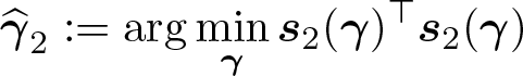
The second estimator we implement, GMM2, is

$\widehat{{\gamma }_2}:=\arg \underset{\gamma }{\min }\hspace{0.17em}{s}_2{\left(\gamma \right)}^{\top }{s}_2\left(\gamma \right)$

which is of the same form as $\widehat{{\gamma }_1}$ but solves the empirical moment equations

$s_2\left(\gamma \right)={\displaystyle \sum _{i=1}^n{\displaystyle \sum _{i\text{'}=1}^n{\displaystyle \sum _{j=1}^m{\displaystyle \sum _{j\text{'}=1}^m{x}_{ij}\left\{\frac{y_{ij}}{e\left(-x_{i\text{'}j}^{\top }\widehat{\gamma }\right)}\frac{y_{i\text{'}j\text{'}}}{e\left(-x_{ij\text{'}}^{\top }\widehat{\gamma }\right)}-\frac{y_{ij\text{'}}}{e\left(-x_{ij}^{\top }\widehat{\gamma }\right)}\frac{y_{i\text{'}j}}{e\left(-x_{i\text{'}j\text{'}}^{\top }\widehat{\gamma }\right)}\right\}}}}}$

The large-sample behavior of this estimator parallels that of $\widehat{{\gamma }_1}$ . The matrices Q ₂ and V ₂ needed to estimate the variance of the limit distribution are readily obtained. We omit further details here for brevity. Other possible estimators can be derived from the conditional moment conditions above. Motivations for the estimators considered here are given in the supplementary material to Jochmans (2017).

The choice between the two estimators depends on the application at hand. The simulation results in Jochmans (2017) show that GMM2 tends to be more efficient than GMM1 in designs where the conditional variance increases with the conditional mean, while GMM1 is relatively more precise in the other situations. In extensive numerical work, we have found that GMM1 is extremely stable, making it reliable. When the linear index x ^⊤ _ij γ can take on large values, the objective function of GMM2 can have multiple local maximums and regions over which it is fairly flat. This can be understood by noting that s ₂( γ ) can be obtained from s ₁( γ ) by multiplying through the latter’s summand with e{( x _ij + x _i′_j′ + x _i′_j + x _ij′) ^⊤ γ }. This complicates numerical optimization using gradient-based methods such as the Newton algorithm that we use. Our code checks whether a global optimum has been reached by verifying whether the empirical moments are (up to tolerance) equal to zero at the solution and gives a warning if not. If this happens, we suggest to experiment with different starting values or to switch to GMM1 instead.

The large number of terms in s ₁( γ ) and s ₂( γ ) may suggest that evaluation of the objective function is time consuming, making estimation and inference based on them infeasible in large datasets (see, for example, the discussion in Egger and Staub [2016]). This is not the case. Careful inspection and subsequent rearrangement of terms reveals that evaluation of these equations is immediate in any matrix-based language (here, Mata). Additional details on this are provided in the appendix. The same is true for the Jacobian matrices Q ₁ and Q ₂ as well as for the variance estimators V ₁ and V ₂. twexp and twgravity are written for balanced datasets. Implementation of our efficient computations would require adjustment to deal with gaps in the data. The exact form of the adjustment depends on the pattern of missingness of the data and is therefore not easily programmed in a generic manner. Note that merely dropping observations for which information is missing is not sufficient. This is because of the structure of the empirical moments, where each summand depends on quadruples of observations. One may, of course, decide to use brute force evaluation of the criterion in such cases.

3 The twexp and twgravity commands

3.1 Command: twexp

The command twexp is designed for (balanced) n × m panel datasets.

Syntax

twexp has the following syntax:

twexp varlist [ if ] [ in ], indn( varname ) indm( varname ) model( option ) initial( vec )

Options

indn( varname ) declares the cross-sectional dimension of the panel. indn() is required.

indm( varname ) declares the time-series dimension of the panel. indm() is required.

model( option ) determines whether GMM1 or GMM2 is implemented. model() is required.

initial( vec ) specifies the starting value for the numerical optimization; the default is the zero vector.

Output

A table in standard layout reports point estimates, standard errors, z statistics, p-values for the null that the coefficient in question is equal to zero, and 95% confidence intervals for each of the coefficients. The vector of point estimates and their estimated covariance matrix can be recovered by typing matrix list e(b) and matrix list e(V), respectively.

3.2 Command: twgravity

The command twgravity is designed for a cross-section on dyadic interactions between n agents. Agents do not interact with themselves, so y_ii and x _ii are not defined. This is like a panel model with m = n−1. In the vectors and matrices defined in section 2, this requires modifying only the range over which the sums go. To evaluate the criterion function efficiently, however, additional intervention is needed (see the discussion on gaps in the previous section). Therefore, we provide a different command to deal with this case.

Syntax

twgravity has the same syntax as twexp:

twgravity varlist [ if ] [ in ], indn( varname ) indm( varname ) model( option ) initial( vec )

Options

indn( varname ) identifies the first agent in the dyad. indn() is required.

indm( varname ) identifies the second agent in the dyad. indm() is required.

model( option ) determines whether GMM1 or GMM2 is implemented. model() is required.

initial( vec ) specifies the starting value for the numerical optimization; the default is the zero vector.

Output

The screen output has the same form as before.

4 Examples

4.1 Patents and R&D

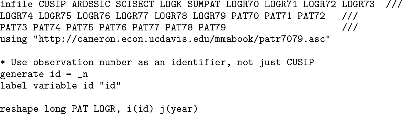
We illustrate the use of twexp by looking at the relationship between the number of patent applications and R&D expenditure. We use the data of Hall, Griliches, and Hausman (1986). The data can be downloaded from the companion website of the Cameron and Trivedi (2005) textbook; ² however, they are not in Stata format. We load them into Stata by typing the following set of commands:

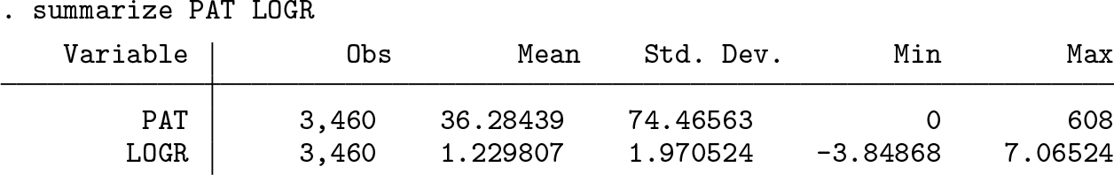
The dataset is a balanced panel on 346 firms and spans the period 1970–1979; note that Cameron and Trivedi (2005) drop all observations for the period 1970–1974, but we do not. For each firm, we have data on the number of patents applied to (PAT) in each year (and were eventually granted) as well as the log of the amount (in 1972 U.S. dollars) spent on R&D during each year (LOGR). A summary of these data is as follows:

It is well established that it is important to control for firm-specific heterogeneity by including firm fixed effects (Hausman, Hall, and Griliches 1984). It also seems important to include a set of time dummies in the specification. These allow to control for aggregate shocks that affect all firms, such as the state of the economy and overall technological progress over time.

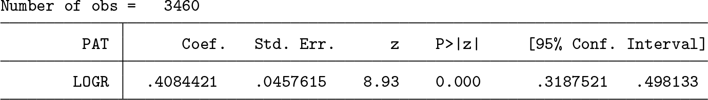
Estimating a two-way exponential regression of PAT on LOGR by means of GMM1 is done by typing

. twexp PAT LOGR, indn(id) indm(year) model(GMM1)

which yields the following output:

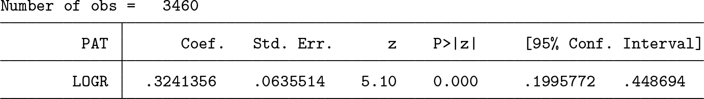
The estimator GMM2 is computed by changing the model() option. For efficiency, we let the optimization start at the point estimate obtained by GMM1. To do so, we first type matrix start = e(b) and next type

. twexp PAT LOGR, indn(id) indm(year) model(GMM2) initial(start)

The output for GMM2 is

4.2 International trade

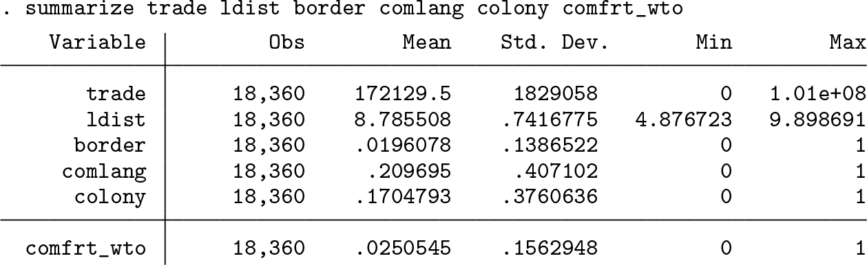
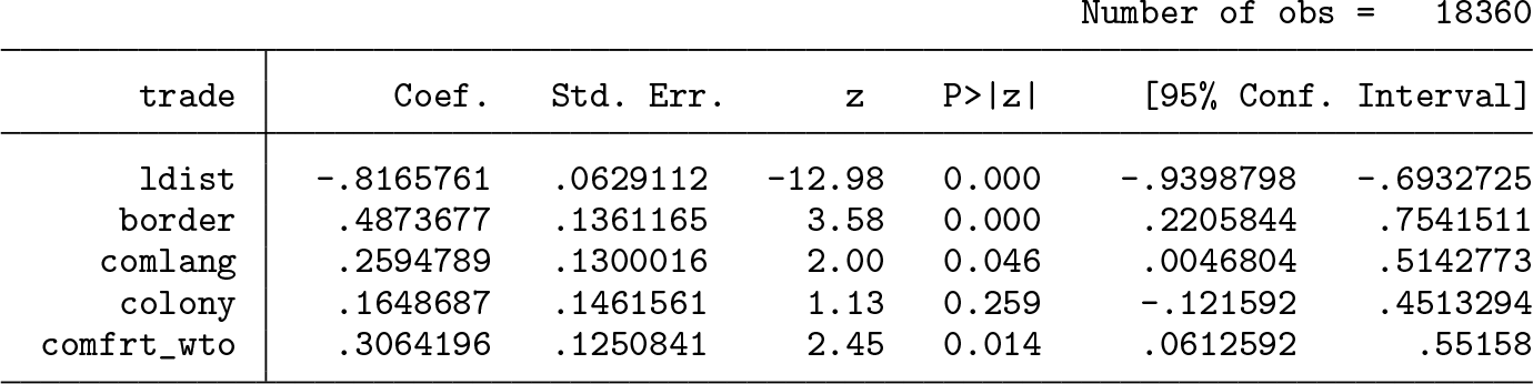
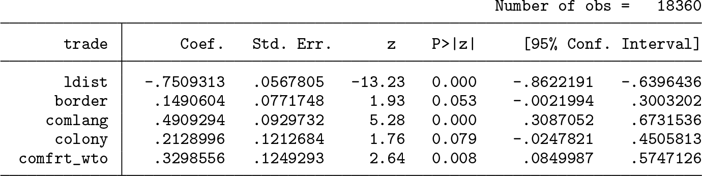
We use the model and data of Santos Silva and Tenreyro (2006) to illustrate the use of twgravity. The dataset can be downloaded from http://personal.lse.ac.uk/tenreyro/lgw.html. The data are a cross-section on bilateral trade flows between 136 countries. The outcome variable is bilateral trade measured in thousands of U.S. dollars (trade). The regressors are all measures of distances between the importing and exporting country. They are (the logarithm of) geographical distance (ldist) and a set of dummies that aim to capture other factors of relatedness. These indicators include whether countries i and j share a common border (border), speak the same language (comlang), have a colonial history (colony), and take part in a common free-trade agreement (comfrt_wto). For each observation, the variables s1_im and s2_ex identify the importer and exporter, respectively.

Fitting this model by GMM1 is done by typing

. twgravity trade ldist border comlang colony comfrt_wto,

> indn(s2_ex) indm(s1_im) model(GMM1)

which completes in 0.81 seconds (using Stata/MP 15.1 on a MacBook 1.4 HGz Intel Core i7 with 16 GB RAM). The following output is reported:

Changing the estimator used to GMM2 is done by typing

. twgravity trade ldist border comlang colony comfrt_wto, indn(s2_ex)

> indm(s1_im) model(GMM2)

which terminates after 1.85 seconds with the following output:

These results correspond to those reported in table 5 of Jochmans (2017). To appreciate the computational speed, note that estimation by PMLE takes just under 16 seconds when using poissonwith dummies, 3.87 seconds when using poi2hdfe, and 1.65 seconds when using ppmlhdfe.

5 Simulations

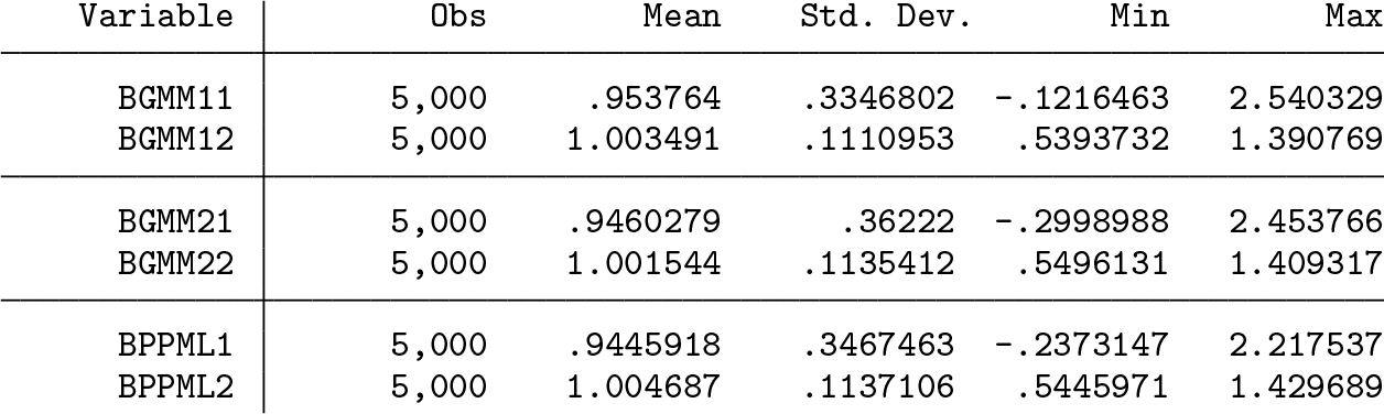
We use simulated data to further illustrate twgravity. The simulation design has two binary regressors. They are independent and take on the value 1 with probability 0.05 and 0.50, respectively. This makes the first regressor sparse. The coefficient on each regressor is set to unity. All fixed effects are set to zero, and errors are drawn from a lognormal distribution such that their logs follow a standard normal distribution. The regressors are drawn once and held fixed across the 5,000 Monte Carlo replications. The errors are redrawn in each replication. The sample size was set to n = 25, yielding 25 × 24 = 600 observations at the dyad level. Simulation results for a variety of other designs and different sample sizes are reported in Jochmans (2017).

The first table below contains summary statistics for the three point estimators considered. BGMM11 refers to the GMM1 point estimator of the first coefficient, and BGMM12 refers to the GMM1 point estimator of the second coefficient. This naming convention is also used for GMM2. BPPML1 and BPPML2 refer to the PMLE point estimates.

All estimators perform well. The average computational efforts for GMM1, GMM2, and PMLE (each starting at a vector of zeros) were 0.1414 seconds, 0.1435 seconds, and 0.1780 seconds, respectively.

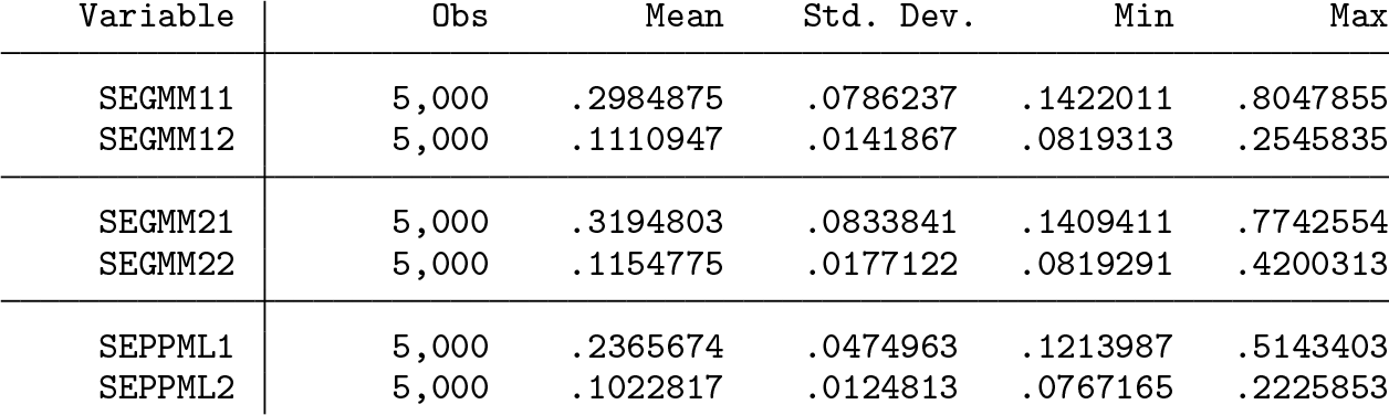
The next table provides corresponding summary statistics for the estimated standard errors for each estimator.

It is of interest to compare the Monte Carlo standard deviation (in the previous table) with the average standard error (in the current table). The ratio of the latter to the former is considerably below unity for PMLE. Thus, the standard errors for the pseudo-Poisson estimator are too small, on average.

6 Conclusion

We have introduced two new commands, twexp and twgravity, for exponential regression models with two-way fixed effects. These estimators are based on Jochmans (2017). They are fast to compute, even in large datasets, and yield reliable standard errors for inference.

References

1.
CameronA. C.TrivediP. K.2005. Microeconometrics: Methods and Applications. New York: Cambridge University Press.
CorreiaS.GuimarãesP.ZylkinT.2019. ppmlhdfe: Stata module for Poisson pseudo-likelihood regression with multiple levels of fixed effects. Statistical Software Components S458622, Department of Economics, Boston College. https://ideas.repec.org/c/boc/bocode/s458622.html.
Fernández-ValI.WeidnerM.2016. Individual and time effects in nonlinear panel models with largeN, T. Journal of Econometrics192: 291–312. https://doi.org/10.1016/j.jeconom.2015.12.014.
6.
GuimarãesP.2016. poi2hdfe: Stata module to estimate a Poisson regression with two high-dimensional fixed effects. Statistical Software Components S457777, Department of Economics, Boston College. https://ideas.repec.org/c/boc/bocode/s457777.html.
7.
HallB. H.GrilichesZ.HausmanJ. A.1986. Patents and R and D: Is there a lag?International Economic Review27: 265–283. https://doi.org/10.2307/2526504.
8.
HausmanJ.HallB. H.GrilichesZ.1984. Econometric models for count data with an application to the patents-R&D relationship. Econometrica52: 909–938. https://doi.org/10.2307/1911191.
PfaffermayrM.2019. Gravity models, PPML estimation and the bias of the robust standard errors
. Applied Economics Letters26: 1467–1471. https://doi.org/10.1080/13504851.2019.1581902.