lassopack: Model selection and prediction with regularized regression in Stata

Abstract

In this article, we introduce lassopack, a suite of programs for regularized regression in Stata. lassopack implements lasso, square-root lasso, elastic net, ridge regression, adaptive lasso, and postestimation ordinary least squares. The methods are suitable for the high-dimensional setting, where the number of predictors p may be large and possibly greater than the number of observations, n. We offer three approaches for selecting the penalization (“tuning”) parameters: information criteria (implemented in lasso2), K-fold cross-validation and h-step-ahead rolling cross-validation for cross-section, panel, and time-series data (cvlasso), and theory-driven (“rigorous” or plugin) penalization for the lasso and square-root lasso for cross-section and panel data (rlasso). We discuss the theoretical framework and practical considerations for each approach. We also present Monte Carlo results to compare the performances of the penalization approaches.

1 Introduction

Machine learning is attracting increasing attention across many scientific disciplines. Recent surveys explore how machine-learning methods can be used in economics and applied econometrics (Varian 2014; Mullainathan and Spiess 2017; Athey 2019; Kleinberg et al. 2018; Athey and Imbens 2019). At the time of writing, Stata offers only a limited set of machine-learning tools. lassopack is an attempt to extend this set by providing easy-to-use and flexible methods for regularized regression in Stata. ¹

While regularized linear regression is only one of many methods in the toolbox of machine learning, it has some properties that make it attractive for empirical research. To begin with, it is a straightforward extension of linear regression. Like ordinary least squares (OLS), regularized linear regression minimizes the sum of squared deviations between observed and model-predicted values but imposes a regularization penalty aimed at limiting model complexity. The most popular regularized regression method is the lasso—which this package is named after—introduced by Frank and Friedman (1993) and Tibshirani (1996), which penalizes the absolute size of coefficient estimates.

The primary purpose of regularized regression, as with supervised machine-learning methods more generally, is prediction. Regularized regression typically does not produce estimates that can be interpreted as causal, and statistical inference on these coefficients is complicated. ² While regularized regression may select the true model as the sample size increases, this is generally the case only under strong assumptions. However, regularized regression can aid causal inference without relying on the strong assumptions required for perfect model selection. The post-double-selection methodology of Belloni, Chernozhukov, and Hansen (2014) and the postregularization approach of Chernozhukov, Hansen, and Spindler (2015) can be used to select appropriate control variables from a large set of putative confounding factors and thereby improve robustness of estimation of the parameters of interest. Likewise, the first stage of two-step least squares is a prediction problem, and lasso or ridge can be applied to obtain optimal instruments (Belloni et al. 2012; Carrasco 2012; Hansen and Kozbur 2014). We implemented these methods in our sister package pdslasso (Ahrens, Hansen, and Schaffer 2018), which builds on the algorithms developed in lassopack.

The strength of regularized regression as a prediction technique stems from the bias-variance tradeoff. The prediction error can be decomposed into the unknown error variance reflecting the overall noise level (which is irreducible), the squared estimation bias, and the variance of the predictor. The variance of the estimated predictor increases with the model complexity, whereas the bias tends to decrease with model complexity. By reducing model complexity and inducing a shrinkage bias, regularized regression methods tend to outperform OLS in terms of out-of-sample prediction performance. In doing so, regularized regression addresses the common problem of overfitting: high in-sample fit (high R ²) but poor prediction performance on unseen data.

Another advantage is that the regularization methods of lassopack—with the exception of ridge regression—set some coefficients to exactly zero, thereby excluding predictors from the model. In this way, regularized regression can serve as a modelselection technique. Model selection is challenging, especially when there are many putative predictors. Iterative testing procedures, such as the general-to-specific approach, typically induce pretesting biases, and hypothesis tests often lead to many false positives. At the same time, high-dimensional problems where the number of predictors is large relative to the sample size are a common phenomenon, especially when the true model is treated as unknown. Regularized regression allows for identification even when the number of predictors exceeds the sample size under the sparsity assumption, which requires that the true model include only a few predictors or, more generally, that only a few predictors are necessary to approximate the true model sufficiently well.

Regularized regression methods rely on tuning parameters that control the degree and type of penalization. lassopack offers three approaches to select these tuning parameters. The classical approach is to select tuning parameters using cross-validation (CV) to optimize out-of-sample prediction performance. CV methods are universally applicable and generally perform well for prediction tasks but are computationally expensive. The second approach relies on information criteria, such as the Akaike information criterion (AIC) (Zou, Hastie, and Tibshirani 2007; Zhang, Li, and Tsai 2010). Information criteria are easy to calculate and have attractive theoretical properties but are less robust to violations of the independence and homoskedasticity assumptions (Arlot and Celisse 2010). The third approach is rigorous penalization for the lasso and squareroot lasso. The tuning parameters are chosen to theoretically provide good prediction performance and control overfitting in the presence of heteroskedastic, non-Gaussian, and cluster-dependent errors (Belloni et al. 2012; Belloni, Chernozhukov, and Wang 2014; Belloni et al. 2016). The rigorous approach places a high priority on controlling overfitting, thus often producing parsimonious models. This strong focus on containing overfitting is practically and theoretically beneficial for selecting control variables or instruments in a structural model but also implies that the approach may be outperformed by CV techniques for pure prediction tasks. Which approach is most appropriate depends on the type of data at hand and the purpose of the analysis. To guide applied researchers, we discuss the theoretical foundation of all three approaches and present Monte Carlo results that assess their relative performance.

This article proceeds as follows. In section 2, we present the estimation methods implemented in lassopack. In sections 3–5, we discuss the aforementioned approaches for selecting the tuning parameters: information criteria in section 3, CV in section 4, and rigorous penalization in section 5. In section 6, we present the three commands, which correspond to the three penalization approaches. In section 7, we demonstrate the commands. In section 8, we present Monte Carlo results. Further technical notes are in section 9.

Notation. We briefly clarify the notation used in this article. Suppose a is a vector of dimension m with typical element a_j for j = 1,…, m. The ℓ ₁ norm is defined as ${\Vert a\Vert }_1={\displaystyle {\sum }_{j=1}^m|a_j|}$ , and the ℓ ₂ norm is ${\Vert a\Vert }_2=\sqrt{{\displaystyle {\sum }_{j=1}^m{|a_j|}^2}}$ . The “ℓ ₀ norm” of a is denoted by || a ||₀ and is equal to the number of nonzero elements in a . $\mathbb{1}\{\cdot \}$ denotes the indicator function. We use the notation b ∨ c to denote the maximum value of b and c, that is, max(b, c).

2 Regularized regression

Here we introduce the regularized regression methods implemented in lassopack. We consider the high-dimensional linear model

$y_i=x_i^{\prime }\beta +{\epsilon }_i,i=1,\dots ,n$

where the number of predictors, p, may be large and even exceed the sample size, n. The regularization methods introduced in this section can accommodate large-p models under the assumption of sparsity: out of the p predictors, only a subset of s ≪ n is included in the true model, where s is the sparsity index

$s:={\displaystyle \sum _{j-1}^p\mathbb{1}}\left\{{\beta }_j\ne 0\right\}={\Vert \beta \Vert }_0$

We refer to this assumption as exact sparsity. It is more restrictive than required, but we use it here for illustration. We will later relax the assumption to allow for nonzero but “small” β_j coefficients. We also define the active set Ω = {j ∊ {1,…, p} : β_j ≠ 0}, which is the set of nonzero coefficients. p, s, Ω, and β may generally depend on n, but we suppress the n subscript for notational convenience.

We adopt the following convention throughout the article: unless otherwise noted, all variables have been mean centered such that ${\displaystyle {\sum }_i{y}_i=0}$ and ${\displaystyle {\sum }_i{x}_{ij}=0}$ , and all variables are measured in their natural units; that is, they have not been prestandardized to have unit variance. By assuming the data have already been mean centered, we simplify the notation and exposition. Leaving the data in natural units, however, allows us to discuss standardization in the context of penalization.

Penalized regression methods rely on tuning parameters that control the degree and type of penalization. The estimation methods implemented in lassopack, which we will introduce in the following subsection, use two tuning parameters; λ controls the general degree of penalization. Setting λ to zero corresponds to no penalization and is equivalent to OLS, while a sufficiently large value of λ yields an empty model, where all coefficients are zero. The second tuning parameter, α, determines the relative contribution of ℓ ₁ (lasso-type) versus ℓ ₂ (ridge-type) penalization. We will discuss the merits and properties of ℓ ₁ and ℓ ₂ penalization in the following subsection. In section 2.2, we introduce the three approaches offered by lassopack for selecting λ and α.

2.1 The estimators

Lasso

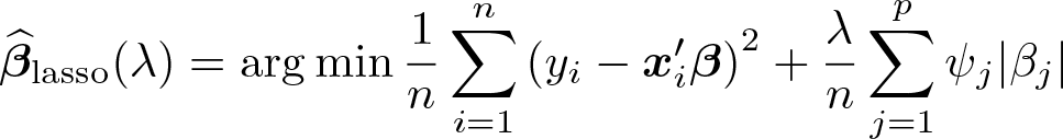
The lasso takes a special position because it provides the basis for the rigorous penalization approach (see section 5) and has inspired other methods such as elastic net and square-root lasso, which we introduce later in this section. The lasso minimizes the mean squared error subject to a penalty on the absolute size of coefficient estimates:

${\widehat{\beta }}_{\text{lasso}}\left(\lambda \right)=\text{arg}\text{min}\frac{1}{n}{\displaystyle \sum _{i=1}^n{\left(y_i-x_i^{\prime }\beta \right)}^2}+\frac{\lambda }{n}{\displaystyle \sum _{j=1}^p{\psi }_j|{\beta }_j|}$

The tuning parameter λ controls the overall penalty level, and ψ_j are predictor-specific penalty loadings.

Tibshirani (1996) motivates the lasso with two major advantages over OLS. First, because of the nature of the ℓ ₁ penalty, the lasso sets some of the coefficient estimates exactly to zero and, in doing so, removes some predictors from the model. Thus, the lasso serves as a model-selection technique and facilitates model interpretation. Second, lasso can outperform least squares in prediction accuracy because of the bias-variance tradeoff.

The lasso coefficient path, which constitutes the trajectory of coefficient estimates as a function of λ, is piecewise linear with changes in slope where variables enter or leave the active set. The change points are referred to as knots.

Unlike OLS, the lasso is not invariant to linear transformations, which is why scaling matters. If the predictors are not of equal variance, the most common approach is to prestandardize the data such that $1/n{\displaystyle {\sum }_i{x}_{ij}^2}=1$ and set ψj = 1 for j = 1,…, p. Alternatively, we can set the penalty loadings to ${\widehat{\psi }}_j={(1/n{\displaystyle {\sum }_i{x}_{ij}^2})}^{-1/2}$ . The two methods yield identical results.

Ridge regression

Ridge regression (Tikhonov 1963; Hoerl and Kennard 1970) replaces the ℓ ₁ penalty of the lasso with an ℓ ₂ penalty, thus minimizing

$\frac{1}{n}{\displaystyle \sum _{i=1}^n{\left(y_i-x_i^{\prime }\beta \right)}^2+\frac{\lambda }{n}}{\displaystyle \sum _{j=1}^p{\psi }_j^2{\beta }_j^2}$

The interpretation and choice of the penalty loadings ψ_j is the same as above. As with the lasso, we need to account for uneven variance either through preestimation standardization or by appropriately choosing the penalty loadings ψ_j .

In contrast with estimators relying on ℓ ₁ penalization, the ridge does not perform variable selection. At the same time, it also does not rely on the assumption of sparsity. This makes the ridge attractive in the presence of dense signals, that is, when the assumption of sparsity does not seem plausible. Dense high-dimensional problems are more challenging than sparse problems; for example, Dicker (2016) shows that, if p/n → ∞, it is not possible to outperform a trivial estimator that includes only the constant. If p, n → ∞ jointly, but p/n converges to a finite constant, the ridge has desirable properties in dense models and tends to perform better than sparsity-based methods (Hsu, Kakade, and Zhang 2014; Dicker 2016; Dobriban and Wager 2018).

Ridge regression is closely linked to principal component regression. Both methods are popular in the context of multicollinearity because of their low variance relative to OLS. Principal component regression applies OLS to a subset of components derived from principal component analysis, thereby discarding a specified number of components with low variance. The rationale for removing low-variance components is that the predictive power of each component tends to increase with the variance. The ridge can be interpreted as projecting the response against principal components while imposing a higher penalty on components exhibiting low variance. Hence, the ridge follows a similar principle, but rather than discarding low-variance components, it applies a more severe shrinkage (Hastie, Tibshirani, and Friedman 2009).

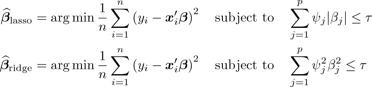
Comparing lasso and ridge regression provides further insights into the nature of ℓ ₁ and ℓ ₂ penalization, so it is helpful to write lasso and ridge in constrained form as

$\begin{array}{l}{\widehat{\beta }}_{\text{lasso}}=\text{ arg min}\frac{1}{n}{\displaystyle \sum _{i=1}^n{\left(y_i-x_i^{\prime }\beta \right)}^2\text{subject to}{\displaystyle \sum _{j=1}^p{\psi }_j|{\beta }_j|}}\le \tau \\ {\widehat{\beta }}_{\text{ridge}}=\text{ arg min}\frac{1}{n}{\displaystyle \sum _{i=1}^n{\left(y_i-x_i^{\prime }\beta \right)}^2\text{subject to}{\displaystyle \sum _{j=1}^p{\psi }_j^2{\beta }_j^2}}\le \tau \end{array}$

and to examine the shapes of the constraint sets. The above optimization problems use the tuning parameter τ instead of λ. Note that there exists a data-dependent relationship between λ and τ.

Figure 1 illustrates the geometry underpinning lasso and ridge regression for the case of p = 2 and ψ ₁ = ψ ₂ = 1 (that is, unity penalty loadings). The gray elliptical lines represent residual sums of squares contours, and the black lines indicate the lasso and ridge constraints. The lasso constraint set, given by |β ₁| + |β ₂| ≤ τ, is diamond shaped with vertices along the axes, from which it immediately follows that the lasso solution may set coefficients exactly to 0. In contrast, the ridge constraint set, ${\beta }_1^2+{\beta }_2^2\le \tau$ , is circular and will thus (effectively) never produce a solution with any coefficient set to 0. Finally, ${\widehat{\beta }}_0$ in the figure denotes the solution without penalization, which corresponds to OLS. The lasso solution at the corner of the diamond implies that, in this example, one of the coefficients is set to zero, whereas ridge and OLS produce nonzero estimates for both coefficients.

Figure 1.

Behavior of ℓ ₁ and ℓ ₂ penalties in comparison. The gray lines represent residual sum of squares contour lines, and the black lines represent the lasso and ridge constraints, respectively. ${\widehat{\beta }}_{\text{OLS}}$ denotes the OLS estimates. ${\widehat{\beta }}_{\text{lasso}}$ and ${\widehat{\beta }}_{\text{ridge}}$ are the lasso and ridge estimates. The illustration is based on Tibshirani (1996, fig. 2).

While there exists no closed-form solution for the lasso, the ridge solution can be expressed as

${\widehat{\beta }}_{\text{ridge}} ={\left(X^{\prime }X+\lambda {\Psi }^{\prime }\Psi \right)}^{-1}{X}^{\prime }y$

Here X is the n × p matrix of predictors with typical element x_ij , y is the response vector, and Ψ = diag(ψ ₁ ,…, ψ_p ) is the diagonal matrix of penalty loadings. The ridge regularizes the regressor matrix by adding positive constants to the diagonal of X ^′ X . The ridge solution is thus generally well defined as long as all the ψ_j and λ are sufficiently large, even if X ^′ X is rank deficient.

Elastic net

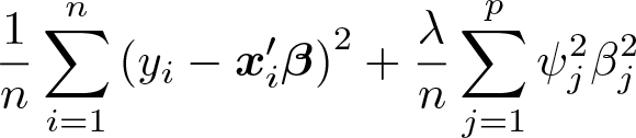
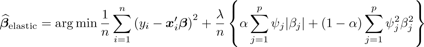
The elastic net of Zou and Hastie (2005) combines some of the strengths of lasso and ridge regression. It applies a mix of ℓ ₁ (lasso-type) and ℓ ₂ (ridge-type) penalization:

${\widehat{\beta }}_{\text{elastic}}=\arg \min \frac{1}{n}{\displaystyle \sum _{i=1}^n{\left(y_i-x_i^{\prime }\beta \right)}^2+\frac{\lambda }{n}}\left\{\alpha {\displaystyle \sum _{j=1}^p{\psi }_j|{\beta }_j|+\left(1-\alpha \right){\displaystyle \sum _{j=1}^p{\psi }_j^2{\beta }_j^2}}\right\}$

The additional parameter α determines the relative contribution of ℓ ₁ versus ℓ ₂ penalization. In the presence of groups of correlated regressors, the lasso typically selects only one variable from each group, whereas the ridge tends to produce similar coefficient estimates for groups of correlated variables. However, the ridge does not yield sparse solutions, impeding model interpretation. The elastic net can produce sparse solutions for some α that are greater than zero and retains or drops correlated variables jointly.

Adaptive lasso

The irrepresentable condition is shown to be sufficient and (almost) necessary for the lasso to be model-selection consistent (Zhao and Yu 2006; Meinshausen and Bühlmann 2006). However, the irrepresentable condition imposes strict constraints on the degree of correlation between predictors in the true model and predictors outside the model. Motivated by this nontrivial condition for the lasso to be variable-selection consistent, Zou (2006) proposed the adaptive lasso. The adaptive lasso uses the penalty loadings of ${\psi }_j=\text{1/}{|{\widehat{\beta }}_{0,j}|}^{\theta }$ , where ${\widehat{\beta }}_{0,j}$ is an initial estimator. The adaptive lasso is variable-selection consistent for a fixed p under weaker assumptions than the standard lasso. If p < n, OLS can be used as the initial estimator. Huang, Ma, and Zhang (2008) prove variable-selection consistency for a large p and suggest using univariate OLS if p > n. The idea of adaptive penalty loadings can also be applied to elastic net and ridge regression (Zou and Zhang 2009).

Square-root lasso

The square-root lasso,

${\widehat{\beta }}_{\sqrt{\text{lasso}}}=\arg \min \sqrt{\frac{1}{n}{\displaystyle \sum _{i=1}^n{\left(y_i-x_i^{\prime }\beta \right)}^2}}+\frac{\lambda }{n}{\displaystyle \sum _{j=1}^p{\psi }_j|{\beta }_j|}$

is a modification of the lasso that minimizes the root mean squared error (rmse) while also imposing an ℓ ₁ penalty. The main advantage of the square-root lasso over the standard lasso becomes apparent if theoretically grounded, data-driven penalization is used. Specifically, the score vector, and thus the optimal penalty level, is independent of the unknown error variance under homoskedasticity as shown by Belloni, Chernozhukov, and Wang (2011), resulting in a simpler procedure for choosing λ (see section 5). ³

Postestimation OLS

Penalized regression methods induce an attenuation bias that can be alleviated by postestimation OLS, which applies OLS to the variables selected by the first-stage variable-selection method, that is,

${\widehat{\beta }}_{\text{post}}=\arg \min \frac{1}{n}{\displaystyle \sum _{i=1}^n{\left(y_i-x_i^{\prime }\beta \right)}^2\hspace{0.17em}\hspace{0.17em}\text{subject to}\hspace{0.17em}\hspace{0.17em}\hspace{0.17em}{\beta }_j=0\hspace{0.17em}\text{if}\hspace{0.17em}}{\tilde{\beta }}_j=0$

where ${\tilde{\beta }}_j$ is a sparse first-step estimator such as the lasso. Thus, postestimation OLS treats the first-step estimator as a genuine model-selection technique. For lasso with theory-driven regularization, Belloni and Chernozhukov (2013) have shown that postestimation OLS, also referred to as postlasso, achieves the same convergence rates as the lasso and can outperform the lasso in situations where consistent model selection is feasible (see also Belloni et al. [2012]). Similar results hold for the square-root lasso (Belloni, Chernozhukov, and Wang 2011, 2014).

2.2 Choice of the tuning parameters

Because coefficient estimates and the set of selected variables depend on λ and α, a central question is how to choose these tuning parameters. Which method is most appropriate depends on the objectives and setting, particularly the aim of the analysis (prediction or model identification), computational constraints, and if and how the independent and identically distributed (i.i.d.) assumption is violated. lassopack offers three approaches for selecting the penalty level of λ and α:

• 1. Information criteria: The value of λ can be selected using information criteria. lasso2 implements model selection using four information criteria. See section 3.

• 2. CV: The aim of CV is to optimize the out-of-sample prediction performance. CV is implemented in cvlasso, which allows for CV across both λ and the elastic-net parameter α. See section 4.

• 3. Theory driven (“rigorous”): Theoretically justified and feasible penalty levels and loadings are available for the lasso and square-root lasso via rlasso. The penalization is chosen to dominate the noise of the data-generating process (represented by the score vector), which allows derivation of theoretical results with regard to consistent prediction and parameter estimation. See section 5.

3 Tuning parameter selection using information criteria

Information criteria are closely related to regularization methods. The classical aic (Akaike 1974) is defined as −2 × log likelihood + 2p. Thus, the AIC can be interpreted as penalized likelihood, which imposes a penalty on the number of predictors included in the model. However, this form of penalization, referred to as the ℓ ₀ penalty, has an important practical disadvantage. To find the model with the lowest AIC, we need to estimate all different model specifications. In practice, it is often not feasible to consider the full model space. For example, with only 20 predictors, there are more than 1,000,000 different models.

The advantage of regularized regression is that it provides a data-driven method for reducing model selection to a one-dimensional problem (or two-dimensional problem in the case of the elastic net) where we need to select λ (and α). Theoretical properties of information criteria are well understood, and they are easy to compute once coefficient estimates are obtained. Thus, it seems natural to use the strengths of information criteria as model-selection procedures to select the penalization level.

Information criteria can be categorized based on two central properties: loss efficiency and model-selection consistency. A model-selection procedure is loss efficient if it yields the smallest averaged squared error attainable by all candidate models. Model-selection consistency requires that the true model be selected with probability approaching 1 as n → ∞. Accordingly, which information criteria is appropriate in a given setting also depends on whether the aim of analysis is prediction or identification of the true model.

We first consider the most popular information criteria, AIC and Bayesian information criterion (Schwarz 1978, BIC):

$\begin{array}{l}\text{AIC}\left(\lambda ,\alpha \right)=n\hspace{0.17em}\text{log}\left\{{\widehat{\sigma }}^2(\lambda , \alpha )\right\}+2\text{df}(\lambda ,\alpha ),\hfill \\ \text{BIC}\left(\lambda ,\alpha \right)=n\hspace{0.17em}\text{log}\left\{{\widehat{\sigma }}^2(\lambda , \alpha )\right\}+\text{df}(\lambda ,\alpha )\hspace{0.17em}\text{log}(n)\hfill \end{array}$

${\widehat{\sigma }}^2\left(\lambda ,\alpha \right)=n^{-1}{\displaystyle {\sum }_{i=1}^n{\widehat{\epsilon }}_i^2}$ and ${\widehat{\epsilon }}_i$ are the residuals. df(λ, α) is the effective degrees of freedom, which is a measure of model complexity. In the linear regression model, the degrees of freedom is simply the number of regressors. Zou, Hastie, and Tibshirani (2007) show that the number of coefficients estimated to be nonzero, sb, is an unbiased and consistent estimate of df(λ) for the lasso (α = 1). Tibshirani and Taylor (2012) confirm that the result also holds if p > n. More generally, the degrees of freedom of the elastic net can be calculated as the trace of the projection matrix; that is,

$\widehat{\text{df}}\left(\lambda ,\alpha \right)=\text{tr}\left[X_{\widehat{\Omega }}{\left\{{X^{\prime }}_{\widehat{\Omega }}{X}_{\widehat{\Omega }}+\lambda \left(1-\alpha \right)\Psi \right\}}^{-1}{X^{\prime }}_{\widehat{\Omega }}\right]$

where $X_{\widehat{\Omega }}$ is the $n\times \widehat{s}$ matrix of selected regressors. The unbiased estimator of the degrees of freedom provides a justification for using the classical AIC and BIC to select tuning parameters (Zou, Hastie, and Tibshirani 2007).

The BIC is known to be model-selection consistent if the true model is among the candidate models, whereas AIC is inconsistent. Clearly, the assumption that the true model is among the candidates is strong; even the existence of the “true model” may be problematic, so loss efficiency may become a desirable second best. The AIC is loss efficient, in contrast with the BIC. Yang (2005) shows that the differences between AIC-type information criteria and BIC-type information criteria are fundamental: a consistent model-selection method such as the BIC cannot be loss efficient, and vice versa. Zhang, Li, and Tsai (2010) confirm this relation in the context of penalized regression.

Both AIC and BIC are not suitable in the large-p–small-n context, where they tend to select too many variables (see Monte Carlo simulations in section 8). It is well known that the AIC is biased in small samples, which motivated the bias-corrected AIC (Sugiura 1978; Hurvich and Tsai 1989),

${\text{AIC}}_c\left(\lambda , \alpha \right)=n\text{log}\left\{{\widehat{\sigma }}^2(\lambda , \alpha )\right\}+2\text{df}(\lambda ,\alpha )\frac{n}{n-\text{df}(\lambda ,\alpha )}$

The bias can be severe if df is large relative to n, and thus the AIC _c should be favored when n is small or with high-dimensional data.

The BIC relies on the assumption that each model has the same prior probability. This assumption seems reasonable when the researcher has no prior knowledge, yet it contradicts the principle of parsimony and becomes problematic if p is large. To see why, consider the case where p = 1000 (following Chen and Chen [2008]): There are 1,000 models for which one parameter is nonzero (s = 1), while there are 1000 × 999/2 models for which s = 2. Thus, the prior probability of s = 2 is greater than the prior probability of s = 1 by a factor of 999/2. More generally, because the prior probability that s = j is greater than the probability that s = j − 1 (up to the point where j = p/2), the BIC is likely to overselect variables. To address this shortcoming, Chen and Chen (2008) introduce the extended BIC (EBIC), defined as

${\text{EBIC}}_{\xi }\left(\lambda ,\alpha \right)=n\text{log}\left\{{\widehat{\sigma }}^2\left(\lambda ,\alpha \right)\right\}+\text{df}\left(\lambda ,\alpha \right)\text{log}(n)+2\xi \text{df}\left(\lambda ,\alpha \right)\text{log}(p)$

which imposes an additional penalty on the size of the model. The prior distribution is chosen such that the probability of a model with dimension j is inversely proportional to the total number of models for which s = j. The additional parameter, ξ ∊ [0, 1], controls the size of the additional penalty. ⁴ Chen and Chen (2008) show in simulation studies that the EBIC _ξ outperforms the traditional BIC, which exhibits a higher false-discovery rate when p is large relative to n.

4 Tuning parameter selection using CV

The aim of CV is to directly assess the performance of a model on unseen data. To this end, the data are repeatedly divided into a training and a validation dataset. The models are fit to the training data, and the validation data are used to assess the predictive performance. In the context of regularized regression, CV can be used to select the tuning parameters that yield the best performance, for example, the best out-of-sample mean squared prediction error. Many methods for CV are available. For an extensive review, we recommend Arlot and Celisse (2010). The most popular method is K-fold CV, which we introduce in section 4.1. In section 4.2, we discuss methods for CV in the time-series setting.

4.1 K-fold CV

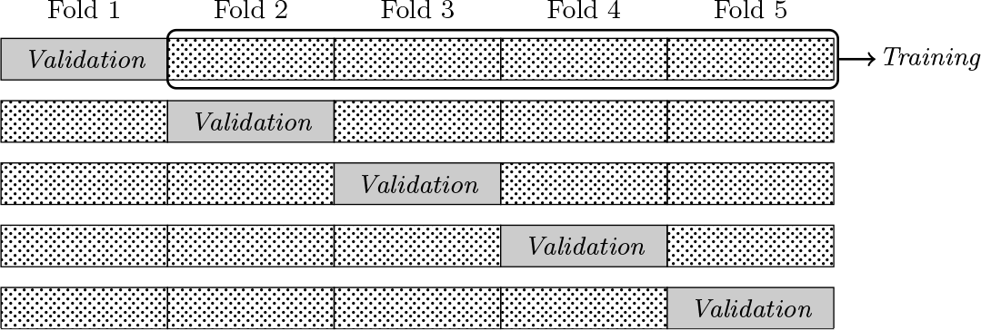
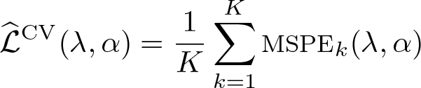
For K-fold CV, proposed by Geisser (1975), the data are split into K groups of approximately equal size that are referred to as folds. Let K _k denote the set of observations in the kth fold, and let n_k be the size of data partition k for k = 1,…, K. In the kth step, the kth fold is treated as the validation dataset, and the remaining K − 1 folds constitute the training dataset. The model is fit to the training data for a given value of λ and α. The resulting estimate, which is based on all the data except the observations in fold k, is ${\stackrel{⌢}{\beta }}_k\left(\lambda ,\alpha \right)$ . The procedure is repeated for each fold, as illustrated in figure 2, so that every data point is used for validation once. The mean squared prediction error (MSPE) for each fold is computed as

${\text{MSPE}}_k\left(\lambda ,\alpha \right)=\frac{1}{n_k}{{\displaystyle \sum _{i\in K_k}\left\{y_i-x_i^{\prime }{\widehat{\beta }}_k\left(\lambda ,\alpha \right)\right\}}}^2$

Figure 2.

Data partition for five-fold CV. Each row corresponds to one step, and each column corresponds to one data partition (“fold”). In the first step, fold 1 constitutes the validation data, and folds 2–5 are the training data.

The K-fold CV estimate of the MSPE, which serves as a measure of prediction performance, is

${\widehat{L}}^{\text{CV}}\left(\lambda ,\alpha \right)=\frac{1}{K}{\displaystyle \sum _{k=1}^K{\text{MSPE}}_k\left(\lambda ,\alpha \right)}$

This suggests selecting λ and α as the values that minimize ${\widehat{L}}^{\text{CV}}\left(\lambda ,\alpha \right)$ . An alternative common rule is to use the largest value of λ that is within one standard deviation of the minimum, which leads to a more parsimonious model.

CV can be computationally expensive. It is necessary to compute ${\widehat{L}}^{\text{CV}}$ for each value of λ on a grid if α is fixed (for example, when using the lasso) or, in the case of the elastic net, for each combination of values of λ and α on a two-dimensional grid. In addition, the model must be fit K times at each grid point such that the computational cost is approximately proportional to K. ⁵

Standardization adds another layer of computational cost to K-fold CV. An important principle in CV is that the training dataset should not contain information from the validation dataset. This mimics the real-world situation where out-of-sample predictions are made despite the true response being unknown. The principle applies not only to individual observations but also to data transformations such as mean centering and standardization. Specifically, data transformations applied to the training data should not use information from the validation data or full dataset. Mean centering and standardization using sample means and sample standard deviations for the full sample would violate this principle. Instead, when in each step the model is fit to the training data for a given λ and α, the training dataset must be recentered and restandardized, or if standardization is built into the penalty loadings, the ${\widehat{\psi }}_j$ must be recalculated based on the training dataset.

The choice of K is a practical problem, but it also has theoretical implications. The variance of ${\widehat{L}}^{\text{CV}}$ decreases with K and is minimal (for linear regression) if K = n, which is referred to as LOO CV. Similarly, the bias decreases with the size of the training dataset. Given computational constraints, K values between 5 and 10 are often recommended, arguing that the performance of CV rarely improves for K values greater than 10 (Hastie, Tibshirani, and Friedman 2009; Arlot and Celisse 2010).

If the aim of the researcher’s analysis is model identification rather than prediction, the theory requires training data to be “small” and the evaluation sample to be close to n (Shao 1993, 1997). The reason is that more data are required to evaluate which model is the “correct” one rather than to decrease bias and variance. This is referred to as the CV paradox (Yang 2006). However, because K-fold CV sets the size of the training sample to approximately n/K, K-fold CV is necessarily ill suited for selecting the true model.

Regarding the K-fold cross-validated lasso, Chetverikov, Liao, and Chernozhukov (2019) demonstrate that the estimation error converges at a near-optimal rate to zero. For example, if the errors are Gaussian, then the convergence rate is slower by a “small logarithmic factor” of $\sqrt{\text{log}\left(np\right)}$ relative to the theory-driven approach of regularization (to be discussed in section 5). The authors also confirm through simulations and deriving sparsity bounds that choosing the tuning parameter by CV tends to yield more predictors than are in the true model and than when theory-driven regularization is used.

4.2 CV with time-series data

Serially dependent data violate the principle that training and validation data are independent. That said, standard K-fold CV may still be appropriate in certain circumstances. Bergmeir, Hyndman, and Koo (2018) show that K-fold CV remains valid in the pure autoregressive model if one is willing to assume that the errors are uncorrelated. A useful implication is that K-fold CV can be used on autoregressive models that include a sufficient number of lags and are not otherwise badly misspecified, because such models have uncorrelated errors.

Rolling h-step-ahead CV is an intuitively appealing approach that directly incorporates the ordered nature of time-series data (Hyndman and Athanasopoulos 2012). ⁶ The procedure builds on repeated h-step-ahead forecasts. The procedure is implemented in lassopack and illustrated in figures 3–4.

Figure 3.

Rolling h-step-ahead CV with expanding training window. T and V denote that the observation is included in the training and validation samples, respectively. A dot (·) indicates that an observation is excluded from both training and validation data.

Figure 4.

Rolling h-step-ahead CV with fixed training window

Figure 3(a) corresponds to the default case of one-step-ahead CV. T denotes the observation included in the training sample, and V refers to the validation sample. In the first step, observations 1–3 constitute the training dataset, and observation 4 is the validation point, whereas the remaining observations are unused as indicated by a dot (·). Figure 3(b) illustrates the case of two-step-ahead CV. In both cases, the training window expands incrementally, whereas figure 4 displays rolling CV with a fixed estimation window.

4.3 Comparison with information criteria

Because information-based approaches and CV share the aim of model selection, one might expect that the two methods share some theoretical properties. Indeed, AIC and LOO CV are asymptotically equivalent, as shown by Stone (1977) for fixed p. Because information criteria require the model to be fit only once, they are computationally much more attractive, which might suggest that information criteria are superior in practice. However, some advantages of CV are its flexibility and that it adapts better to situations where the assumptions underlying information criteria, for example, homoskedasticity, are not satisfied (Andrews 1991; Arlot and Celisse 2010). If the aim of the analysis is identifying the true model, BIC and EBIC provide a better choice than K-fold CV, because there are strong but well-understood conditions under which BIC and EBIC are model-selection consistent.

5 Rigorous penalization

This section introduces the “rigorous” or plugin approach to penalization. Following Chernozhukov, Hansen, and Spindler (2016), we use the term “rigorous” to emphasize that the framework is grounded in theory in that it provides penalization parameters that guarantee optimal rate of convergence for prediction and parameter estimation. The approach also yields models whose size is of the same order as the true model. Rigorous penalization is of special interest because it provides the basis for methods to facilitate causal inference in the presence of many instruments, many control variables, or both; these methods are the instrumental-variables lasso (Belloni et al. 2012), the post-double-selection estimator (Belloni, Chernozhukov, and Hansen 2014), and the postregularization estimator (Chernozhukov, Hansen, and Spindler 2015), all of which are implemented in our sister package pdslasso (Ahrens, Hansen, and Schaffer 2018).

We discuss the conditions required to derive theoretical results for the lasso in section 5.1. Sections 5.2–5.5 present feasible algorithms for rigorous penalization choices for the lasso and square-root lasso under i.i.d., heteroskedastic, and cluster-dependent errors. Section 5.6 presents a related test for joint significance testing.

5.1 Theory of the lasso

There are three main conditions required to guarantee that the lasso is consistent in terms of prediction and parameter estimation. ⁷ The first condition relates to sparsity. Sparsity is an attractive assumption in settings where we have a large set of potentially relevant regressors or consider various model specifications but assume that only one true model exists that includes few regressors. We have introduced exact sparsity in section 2, but the assumption is stronger than needed. For example, some true coefficients may be nonzero but small in absolute size, in which case it might be preferable to omit them, so we use a weaker assumption:

Approximate sparsity. Belloni et al. (2012) consider the approximate sparse model

$y_i=f\left(w_i\right)+{\epsilon }_i=x_i^{\prime }{\beta }_0+r_i+{\epsilon }_i$

The elementary regressors w _i are linked to the dependent variable through the unknown and possibly nonlinear function f(·). The aim of lasso (and square-root lasso) estimation is to approximate f( w _i ) using the target parameter vector β ₀ and the transformations x _i := P ( w _i ), where P (·) denotes a dictionary of transformations. The vector x _i may be large relative to the sample size either because w _i itself is high dimensional and x _i := w _i or because many transformations such as dummies, polynomials, or interactions a re considered to approximate f( w _i ).

The assumption of approximate sparsity requires the existence of a target vector β ₀, which ensures that f( w _i ) can be approximated sufficiently well while using only few nonzero coefficients. Specifically, the target vector β ₀ and the sparsity index s are assumed to meet the condition

${\Vert {\beta }_0\Vert }_0:=s\ll n\text{with}\frac{s^2{\log }^2\left(p\vee n\right)}{n}\to 0$

and the resulting approximation error, $r_i=f(w_i)-x_i^{\prime }{\beta }_0$ , is bounded such that

$\sqrt{\frac{1}{n}{\displaystyle \sum _{i=1}^n{r}_i^2}}\le C\sqrt{\frac{s}{n}}$

1

where C is a positive constant. To emphasize the distinction between approximate and exact sparsity, consider the special case where f( w _i ) is linear with $f(w_i)-x_i^{\prime }{\beta }^{\star }$ but where the true parameter vector β ^⋆ violates exact sparsity so that ||β ^⋆||₀ > n. If β ^⋆ has many elements that are negligible in absolute size, we might still be able to approximate β ^⋆ using the sparse target vector β ₀ as long as $r_i=x_i^{\prime }\left({\beta }^{\star }-{\beta }_0\right)$ is sufficiently small as specified in (1).

Restricted sparse eigenvalue condition. The second condition relates to the Gram matrix, n^{− 1} X ^′ X . In the high-dimensional setting where p is larger than n, the Gram matrix is necessarily rank deficient, and the minimum (unrestricted) eigenvalue is zero, that is,

$\underset{\mathit{\delta }\ne \text{0}}{\min }{\frac{{\Vert \mathit{X}\mathit{\delta }\Vert }_2}{\sqrt{n}\Vert \mathit{\delta }\Vert }}_2=0$

Thus, to accommodate a large p, the full-rank condition of OLS needs to be replaced by a weaker condition. In the context of sparse models, we instead assume that “small” submatrices of size m, where m is slightly larger than s, are well behaved. This is in fact the restricted sparse eigenvalue condition (RSEC) of Belloni et al. (2012). The RSEC formally states that the minimum sparse eigenvalues

${\varphi }_{\min }\left(m\right)=\underset{1\le {\Vert \mathit{\delta }\Vert }_0\le m}{\min }\frac{{\mathit{\delta }}^{\prime }{\mathit{X}}^{\prime }\mathit{X}\mathit{\delta }}{{\Vert \mathit{\delta }\Vert }_2^2}\text{and}{\varphi }_{\max }\left(m\right)=\underset{1\le {\Vert \mathit{\delta }\Vert }_0\le m}{\max }\frac{{\mathit{\delta }}^{\prime }{\mathit{X}}^{\prime }\mathit{X}\mathit{\delta }}{{\Vert \mathit{\delta }\Vert }_2^2}$

are bounded away from zero and from above. The requirement φ _min(m) > 0 implies that all small submatrices of size m have to be positive definite. ⁸

Regularization event. The third central condition concerns the choice of the penalty level λ and the predictor-specific penalty loadings ψ_j . The idea is to select the penalty parameters to control the random part of the problem in that

$\frac{\lambda }{n}\ge c\underset{1\le j\le p}{\max }|{\psi }_j^{-1}{S}_j|\text{where}{\text{S}}_j=\frac{2}{n}{\displaystyle \sum _{i=1}^n{x}_{ij}{\epsilon }_i}$

2

with high probability. Here c > 1 is a constant slack parameter, and S_j is the jth element of the score vector $S=\nabla \widehat{Q}\left(\beta \right)$ , which is the gradient of $\widehat{Q}$ at the true value β . The score vector summarizes the noise associated with the estimation problem.

Denote by $\Lambda =n{\max }_j|{\psi }_j^{-1}{S}_j|$ the maximal element of the score vector scaled by n and ψ_j , and denote by q _Λ(·) the quantile function for Λ. ⁹ In the rigorous lasso, we choose the penalty parameters λ and ψ_j and confidence level γ so that

$\lambda \ge c{q}_{\Lambda }\left(1-\gamma \right)$

3

A simple example illustrates the intuition behind this approach. Consider the case where the true model has β_j = 0 for j = 1,…, p; that is, none of the regressors appears in the true model. It can be shown that for the lasso to select no variables, the penalty parameters λ and ψ_j need to satisfy $\lambda \ge 2{\max }_j|{\displaystyle {\sum }_i{\psi }_j^{-1}{x}_{ij}{y}_i}|$ . ¹⁰ This is because none of the regressors appears in the true model, y_i = ε_i . We can therefore rewrite the requirement for the lasso to correctly identify the model without regressors as $\lambda \ge 2{\max }_j|{\displaystyle {\sum }_i{\psi }_j^{-1}{x}_{ij}{\epsilon }_i}|$ , which is the regularization event in (2). We want this regularization event to occur with a high probability of at least (1 − γ). If we choose values for λ and ψ_j such that λ ≥ q _Λ(1−γ), then by the definition of a quantile function, we will choose the correct model (no regressors) with a probability of at least (1 − γ). This is simply the rule in (3).

The chief practical problem in using the rigorous lasso is that the quantile function q _Λ(·) is unknown. There are two approaches to addressing this problem proposed in the literature, both of which are implemented in rlasso. The rlasso default is the “asymptotic” or X-independent approach: theoretically grounded and feasible penalty level and loadings are used that guarantee that (2) holds asymptotically, because n → ∞ and γ → 0. The X-independent penalty-level choice can be interpreted as an asymptotic upper bound on the quantile function q _Λ(·). In the “exact” or X-dependent approach, the quantile function q _Λ(·) is directly estimated by simulating the distribution of q _Λ(1− γ| X ), the (1−γ)-quantile of Λ conditional on the observed regressors X . We first focus on the X-independent approach and introduce the X-dependent approach in section 5.5.

5.2 Rigorous lasso

Belloni et al. (2012) show—using moderate deviation theory of self-normalized sums from Jing, Shao, and Wang (2003)—that the regularization event in (2) holds asymptotically; that is,

$\text{P}\left(\underset{1\le j\le p}{\max }c|S_j|\le \frac{\lambda {\psi }_j}{n}\right)\to 1\text{as}n\to \infty ,\gamma \to 0$

if the penalty levels and loadings are set to

$\begin{array}{ll}\text{homosdasticity:}\hspace{0.17em}\hspace{0.17em}\hspace{0.17em}\hspace{0.17em}\hspace{0.17em}\hspace{0.17em}\hspace{0.17em}\lambda =2c\sigma \sqrt{n}{\Phi }^{-1}\left\{1-\gamma /\left(2p\right)\right\}\hfill & {\psi }_j=\sqrt{\frac{1}{n}{\displaystyle {\sum }_i{x}_{ij}^2}}\hfill \\ \text{heteroskedasticity:}\hspace{0.17em}\hspace{0.17em}\hspace{0.17em}\lambda =2c\sqrt{n}{\Phi }^{-1}\left\{1-\gamma /\left(2p\right)\right\}\hfill & {\psi }_j=\sqrt{\frac{1}{n}{\displaystyle {\sum }_i{x}_{ij}^2{\epsilon }_i^2}}\hfill \end{array}\left(4\right)$

4

under homoskedasticity and heteroskedasticity, respectively. c is the slack parameter from above, and the significance level γ is required to converge toward 0. rlasso uses c = 1.1 and γ = 0.1/ log(n) as defaults. ^{11 , 12}

Homoskedasticity. We first focus on the case of homoskedasticity. In the rigorouslasso approach, we standardize the score. But because $E\left(x_{ij}^2{\epsilon }_i^2\right)={\sigma }^{2}E\left(x_{ij}^2\right)$ under homoskedasticity, we can separate the problem into two parts: the regressor-specific penalty loadings ${\psi }_j=\sqrt{\left(1/n\right){\displaystyle {\sum }_i{x}_{ij}^2}}$ standardize the regressors, and σ moves into the overall penalty level. In the special case where the regressors have already been standardized such that $\left(1/n\right){\displaystyle {\sum }_i{x}_{ij}^2}=1$ , the penalty loadings are ψ_j = 1. Hence, the purpose of the regressor-specific penalty loadings in the case of homoskedasticity is to accommodate regressors with unequal variance.

The only unobserved term is σ, which appears in the optimal penalty level λ. To estimate σ, we can use some initial set of residuals ${\widehat{\epsilon }}_{0,i}$ and calculate the initial estimate as ${\widehat{\sigma }}_0=\sqrt{\left(1/n\right){\displaystyle {\sum }_i{\widehat{\epsilon }}_{0,i}^2}}$ . A possible choice for the initial residuals is ${\widehat{\epsilon }}_{0,i}=y_i$ as in Belloni et al. (2012) and Belloni, Chernozhukov, and Hansen (2014). rlasso uses the OLS residuals ${\widehat{\epsilon }}_{0,i}=y_i-x_i{\left[D\right]}^{\prime }{\widehat{\beta }}_{\text{OLS}}$ , where D is the set of five regressors exhibiting the highest absolute correlation with y_i . ¹³ The procedure is summarized in algorithm A:

□ Algorithm A: Estimation of penalty level under homoskedasticity

• 1. Set k = 0, and define the maximum number of iterations, K. Regress y_i against the subset of d predictors exhibiting the highest correlation coefficient with y_i , and compute the initial residuals as ${\widehat{\epsilon }}_{0,i}={\widehat{\epsilon }}_{k,i}=y_i-x_i{\left[D\right]}^{\prime }{\widehat{\beta }}_{\text{OLS}}$ . Calculate the homoskedastic penalty loadings in (4).

• 2. If k ≤ K, compute the homoskedastic penalty level in (4) by replacing σ with ${\widehat{\sigma }}_k=\sqrt{(1/n){\displaystyle {\sum }_i{\widehat{\epsilon }}_{k,i}^2}}$ , and obtain the rigorous lasso or postlasso estimator ${\widehat{\beta }}_k$ . Update the residuals ${\widehat{\epsilon }}_{k+1,i}=y_i-x_i^{\prime }{\widehat{\beta }}_k$ . Set k ← k + 1.

• 3. Repeat step 2 until k > K or until convergence by updating the penalty level.

□

The rlasso default is to perform one further iteration after the initial estimate (that is, K = 1), which in our experience provides good performance. Both lasso and postlasso can be used to update the residuals. rlasso uses postlasso to update the residuals. ¹⁴

Heteroskedasticity. The X-independent choice for the overall penalty level under heteroskedasticity is $\lambda =2c\sqrt{n}{\Phi }^{-1}\left\{1-\gamma /(2p)\right\}$ . The only difference from the homoskedastic case is the absence of σ. The variance of ε is now captured via the penalty loadings, which are set to ${\psi }_j=\sqrt{1/n{\displaystyle {\sum }_i{x}_{ij}^2{\epsilon }_i^2}}$ . Hence, the penalty loadings here serve two purposes: accommodating both heteroskedasticity and regressors with uneven variance. To help with intuition, we consider the case where the predictors are already standardized. It is easy to see that, if the errors are homoskedastic with σ = 1, the penalty loadings are (asymptotically) just ψ_j = 1. If the data are heteroskedastic, however, the standardized penalty loading will not be 1. In most practical settings, the usual pattern will be that $\widehat{{\psi }_j}>1$ for some j. Intuitively, heteroskedasticity typically increases the likelihood that the term ${\max }_j|{\displaystyle {\sum }_i{x}_{ij}{\epsilon }_i}|$ takes on extreme values, thus requiring a higher degree of penalization through the penalty loadings. ¹⁵

The disturbances ε_i are unobserved, so we obtain an initial set of penalty loadings ${\widehat{\psi }}_j$ from an initial set of residuals ${\widehat{\epsilon }}_{0,i}$ , similarly to the i.i.d. case above. We summarize the algorithm for estimating the penalty level and loadings as follows:

□ Algorithm B: Estimation of penalty loadings under heteroskedasticity

• 1. Set k = 0, and define the maximum number of iterations, K. Regress y_i against the subset of d predictors exhibiting the highest correlation coefficient with y_i , and compute the initial residuals as ${\widehat{\epsilon }}_{0,i}={\widehat{\epsilon }}_{k,i}=y_i-x_i{\left[D\right]}^{\prime }{\widehat{\beta }}_{\text{OLS}}$ . Calculate the heteroskedastic penalty level λ in (4).

• 2. If k ≤ K, compute the heteroskedastic penalty loadings using the formula given in (4) by replacing ε_i with ${\widehat{\epsilon }}_{k,i}$ , and obtain the rigorous lasso or postlasso estimator ${\widehat{\beta }}_k$ . Update the residuals ${\widehat{\epsilon }}_{k+1,i}=y_i-x_i^{\prime }{\widehat{\beta }}_k$ . Set k ← k + 1.

• 3. Repeat step 2 until k > K or until convergence by updating the penalty loadings.

□

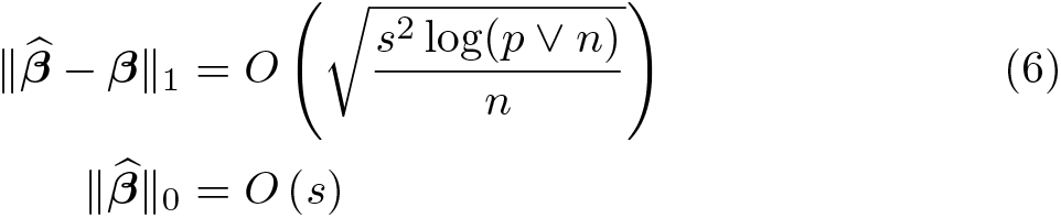
Theoretical property. Under the assumptions of sparse eigenvalue condition and approximate sparse model, and if penalty level λ and the penalty loadings are estimated by algorithm A or B, the lasso and postlasso obey ¹⁶

$\sqrt{\frac{1}{n}{\displaystyle \sum _{i=1}^n{\left(x_i^{\prime }\widehat{\beta }-x_i^{\prime }\beta \right)}^2}}=O\left(\sqrt{\frac{s\log \left(p\vee n\right)}{n}}\right)$

5

$\begin{array}{lll}\hfill {\Vert \widehat{\beta }-\beta \Vert }_1& \hfill =\hfill & O\left(\sqrt{\frac{s^2\log \left(p\vee n\right)}{n}}\right)\hfill \\ \hfill {\Vert \widehat{\beta }\Vert }_0& \hfill =\hfill & O\left(s\right)\hfill \end{array}$

6

The first relation in (5) provides an asymptotic bound for the prediction error, and the second relation in (6) bounds the bias in estimating the target parameter β . Belloni et al. (2012) refer to the above convergence rates as near-oracle rates. If the identity of the s variables in the model were known, the prediction error would converge at the oracle rate $\sqrt{s/n}$ . Thus, the logarithmic term log(p ∨ n) can be interpreted as the cost of not knowing the true model. The final relation is a sparsity bound that shows that the size of the fit model does not diverge relative to the true model.

For comparison, the rates of the rigorous lasso are faster than the convergence rates of the K-fold cross-validated lasso derived in Chetverikov, Liao, and Chernozhukov (2019). Furthermore, the sparsity bound in Chetverikov, Liao, and Chernozhukov (2019) does not rule out situations where $||\widehat{\beta }|{|}_0-s\to \infty$ , implying that the model fit using CV may be much larger than the true model because the penalty level chosen by K-fold CV cannot be guaranteed to satisfy the regularization event in (2). Indeed, Chetverikov, Liao, and Chernozhukov (2019) confirm in simulations that the cross-validated penalty is often smaller than (2) requires.

5.3 Rigorous square-root lasso

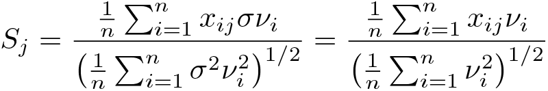
The theory of the square-root lasso is similar to the theory of the lasso (Belloni, Chernozhukov, and Wang 2011; 2014). The jth element of the score vector is now defined as

$S_j=\frac{\frac{1}{n}{\displaystyle {\sum }_{i=1}^n{x}_{ij}{\epsilon }_i}}{{\left(\frac{1}{n}{\displaystyle {\sum }_{i=1}^n{\epsilon }_i^2}\right)}^{1/2}}$

To see why the square-root lasso is of special interest, we define the standardized errors ν_i as ν_i = ε_i/σ. The jth element of the score vector becomes

$S_j=\frac{\frac{1}{n}{\displaystyle {\sum }_{i=1}^n{x}_{ij}\sigma v_i}}{{\left(\frac{1}{n}{\displaystyle {\sum }_{i=1}^n{\sigma }^2{v}_i^2}\right)}^{1/2}}=\frac{\frac{1}{n}{\displaystyle {\sum }_{i=1}^n{x}_{ij}{v}_i}}{{\left(\frac{1}{n}{\displaystyle {\sum }_{i=1}^n{v}_i^2}\right)}^{1/2}}$

and is thus independent of σ. For the same reason, the optimal penalty level for the square-root lasso in the i.i.d. case,

$\lambda =c\sqrt{n}{\Phi }^{-1}\left\{1-\gamma /(2p)\right\}$

7

is independent of the noise level σ.

Homoskedasticity. The ideal penalty loadings under homoskedasticity for the squareroot lasso are given by formula (iv) in table 1, which provides an overview of penaltyloading choices. The ideal penalty parameters are independent of the unobserved error, which is an appealing theoretical property and implies a practical advantage. Because both λ and ψ_j can be calculated from the data, the rigorous square-root lasso is a onestep estimator under homoskedasticity. Belloni, Chernozhukov, and Wang (2011) show that the square-root lasso performs similarly to the lasso with infeasible ideal penalty loadings.

Table 1.

Ideal penalty loadings for the lasso and square-root lasso under homoskedasticity, heteroskedasticity, and cluster dependence

	lasso	square-root lasso
homoskedasticity	(i) $\sqrt{\frac{1}{n}{\displaystyle \sum _{i=1}^n{x}_{ij}^2}}$	(iv) $\sqrt{\frac{1}{n}{\displaystyle \sum _{i=1}^n{x}_{ij}^2}}$
heteroskedasticity	(ii) $\sqrt{\frac{1}{n}{\displaystyle \sum _{i=1}^n{x}_{ij}^2{\epsilon }_i^2}}$	(v) $\sqrt{\frac{1}{n}{\displaystyle \sum _{i=1}^n{x}_{ij}^2}}\vee \sqrt{\frac{{\displaystyle {\sum }_{i=1}^n{x}_{ij}^2{\epsilon }_i^2}}{{\displaystyle {\sum }_{i=1}^n{\epsilon }_i^2}}}$
cluster dependence	(iii) $\sqrt{\frac{1}{nT}{\displaystyle \sum _{i=1}^n{u}_{ij}^2}}$	(vi) $\sqrt{\frac{1}{nT}{\displaystyle \sum _{i=1}^n{\displaystyle \sum _{t=1}^T{x}_{ijt}^2}}}\vee \sqrt{\frac{{\displaystyle {\sum }_{i=1}^n{u}_{ij}^2}}{{\displaystyle {\sum }_{i=1}^n{\displaystyle {\sum }_{t=1}^T{\epsilon }_{it}^2}}}}$

note: Formulas (iii) and (vi) use the notation $u_{ij}={\displaystyle {\sum }_t{x}_{itj}{\epsilon }_{it}}$ .

Heteroskedasticity. In the case of heteroskedasticity, the optimal square-root lasso penalty level remains (7), but the penalty loadings, given by formula (v) in table 1, depend on the unobserved error and need to be estimated. Note that the updated penalty loadings using the residuals ${\widehat{\epsilon }}_i$ use thresholding: the penalty loadings are enforced to be greater than or equal to the loadings in the homoskedastic case. The rlasso default algorithm used to obtain the penalty loadings in the heteroskedastic case is analogous to algorithm B. ¹⁷ While the ideal penalty loadings are not independent of the error term if the errors are heteroskedastic, the square-root lasso may still have an advantage over the lasso because the ideal penalty loadings are pivotal with respect to the error term up to scale, as pointed out above.

5.4 Rigorous penalization with panel data

Belloni et al. (2016) extend the rigorous framework to the case of clustered data, which accommodates a limited form of dependence—within-group correlation—as well as heteroskedasticity. They prove consistency of the rigorous lasso using this approach in the large-n–fixed-T and large-n–large-T settings. The authors present the approach in the context of a fixed-effects panel-data model, $y_{it}={x^{\prime }}_{it}\beta +{\mu }_i+{\epsilon }_{it}$ , and apply the rigorous lasso after the within transformation to remove the fixed effects µ_i . The approach extends to any clustered-type setting and to balanced and unbalanced panels. For convenience, we ignore the fixed effects and write the model as a balanced panel:

$y_{it}={{\mathit{x}}^{\prime }}_{it}\mathit{\beta }+{\epsilon }_{it}\hspace{0.17em}\hspace{0.17em}\hspace{0.17em}i=1,\dots ,n,t=1,\dots ,T$

The intuition behind the Belloni et al. (2016) approach is similar to that behind the clustered standard errors reported by various Stata estimation commands: observations within clusters are aggregated to create “superobservations” that are assumed independent, and these superobservations are treated similarly to cross-sectional observations in the nonclustered case. Specifically, define for the ith cluster and jth regressor the superobservation $u_{ij}:={\displaystyle {\sum }_t{x}_{ijt}{\epsilon }_{it}}$ . Then the penalty loadings for the clustered case are

${\psi }_j=\sqrt{\frac{1}{nT}{\displaystyle \sum _{i=1}^n{u}_{ij}^2}}$

which resembles the heteroskedastic case. The rlasso default for the overall penalty level is the same as in the heteroskedastic case, $\lambda =2c\sqrt{n}{\Phi }^{-1}\left\{1-\gamma /(2p)\right\}$ , except that the default value for γ is 0.1/ log(n); that is, we use the number of clusters n rather than the number of observations nT. lassopack also implements the rigorous square-root lasso for panel data, which uses the overall penalty in (7) and the penalty loadings in formula (vi) in table 1.

5.5 X-dependent lambda

The X-dependent penalty is an alternative, sharper choice for the overall penalty level. Recall that the asymptotic, X-independent choice in (4) can be interpreted as an asymptotic upper bound on the quantile function of Λ, which is the scaled maximum value of the score vector. Instead of using the asymptotic choice, we can estimate by simulation the distribution of Λ conditional on the observed X and use this simulated distribution to obtain the quantile q _Λ(1 − γ| X ).

In the case of estimation by the lasso under homoskedasticity, we simulate the distribution of Λ using the statistic W, defined as

$W=2\widehat{\sigma }\underset{1\le j\le p}{\max }\left|{\displaystyle \sum _{i=1}^n{\psi }_j^{-1}{x}_{ij}{g}_i}\right|$

where ψ_j is the penalty loading for the homoskedastic case, $\widehat{\sigma }$ is an estimate of the error variance using some previously obtained residuals, and g_i is an i.i.d. standard normal variate drawn independently of the data. The X-dependent penalty choice is sharper and adapts to correlation in the regressor matrix (Belloni and Chernozhukov 2011).

Under heteroskedasticity, the lasso X-dependent penalty is obtained by a multiplier bootstrap procedure. In this case, the simulated statistic W is defined as in formula (ii) in table 2. The cluster–robust X-dependent penalty is again obtained analogously to the heteroskedastic case by defining superobservations, and the statistic W is defined as in formula (iii) in table 2. Note that the standard normal variate g_i varies across but not within clusters.

Table 2.

Definition of W statistic for the simulation of the distribution of Λ for the lasso and square-root lasso under homoskedasticity, heteroskedasticity, and cluster dependence

	lasso	square-root lasso
homoskedasticity	(i) $2\widehat{\sigma }\underset{1\le j\le p}{\max }\left|{\displaystyle \sum _{i=1}^n{\psi }_j^{-1}{x}_{ij}{g}_i}\right|$	(iv) $\frac{1}{{\widehat{\sigma }}_g}\underset{1\le j\le p}{\max }\left|{\displaystyle \sum _{i=1}^n{\psi }_j^{-1}{x}_{ij}{g}_i}\right|$
heteroskedasticity	(ii) $2\underset{1\le j\le p}{\max }\left|{\displaystyle \sum _{i=1}^n{\psi }_j^{-1}{x}_{ij}{\widehat{\epsilon }}_i{g}_i}\right|$	(v) $\frac{1}{{\widehat{\sigma }}_g}\underset{1\le j\le p}{\max }\left|{\displaystyle \sum _{i=1}^n{\psi }_j^{-1}{x}_{ij}\widehat{\epsilon }{g}_i}\right|$
cluster dependence	(iii) $2\underset{1\le j\le p}{\max }\left|{\displaystyle \sum _{i=1}^n{\psi }_j^{-1}{\widehat{u}}_{ij}{g}_i}\right|$	(vi) $\frac{1}{{\widehat{\sigma }}_g}\underset{1\le j\le p}{\max }\left|{\displaystyle \sum _{i=1}^n{\psi }_j^{-1}{\widehat{u}}_{ij}{g}_i}\right|$

note: g_i is an i.i.d. standard normal variate drawn independently of the data; ${\widehat{\sigma }}_g=\frac{1}{n}{\displaystyle {\sum }_i{g}_i^2}$ . Formulas (iii) and (vi) use the notation ${\widehat{u}}_{ij}={\displaystyle {\sum }_t{x}_{itj}{\widehat{\epsilon }}_{it}}$ .

The X-dependent penalties for the square-root lasso are similarly obtained from quantiles of the simulated distribution of the square-root lasso Λ and are given by formulas (iv), (v), and (vi) in table 2 for the homoskedastic, heteroskedastic, and clustered cases, respectively. ¹⁸

5.6 Significance testing with the rigorous lasso

Inference using the lasso, especially in the high-dimensional setting, is a challenging and ongoing research area (see footnote 2). A test that has been developed and is available in rlasso corresponds to the test for joint significance of regressors using F or χ ² tests that is common in regression analysis. Specifically, Belloni et al. (2012) suggest using the Chernozhukov, Chetverikov, and Kato (2013, app. M) sup-score test to test for the joint significance of the regressors; that is,

$H_0:{\beta }_1=\cdots ={\beta }_p=0$

As in the preceding sections, regressors are assumed to be mean centered and in their original units.

If the null hypothesis is correct and the rest of the model is well specified, including the assumption that the regressors are orthogonal to the disturbance ε_i , then y_i = ε_i and hence E( x _iε_i ) = E( x _iy_i ) = 0. The sup-score statistic is

$S_{SS}=\sqrt{n}\underset{1\le j\le p}{\max }\left|\frac{1}{n}{\displaystyle \sum _{i=1}^n{\psi }_j^{-1}{x}_{ij}{y}_i}\right|$

8

where ${\psi }_j=\sqrt{\left(1/n\right){\displaystyle {\sum }_{i=1}^n{\left(x_{ij}{y}_i\right)}^2}}$ . Intuitively, the ψ_j in (8) plays the same role as the penalty loadings do in rigorous-lasso estimation.

The p-value for the sup-score test is obtained by a multiplier bootstrap procedure simulating the distribution of S_SS by the statistic W, defined as

$W=\sqrt{n}\underset{1\le j\le p}{\max }\left|\frac{1}{n}{\displaystyle \sum _{i=1}^n{\psi }_j^{-1}{x}_{ij}{y}_i{g}_i}\right|$

where g_i is an i.i.d. standard normal variate drawn indep endently of the data and ψ_j is defined as in (8).

The procedure above is valid under both homoskedasticity and heteroskedasticity but requires independence. A cluster–robust version of the sup-score test that accommodates within-group dependence is

$S_{SS}=\sqrt{nT}\underset{1\le j\le p}{\max }\left|\frac{1}{nT}{\displaystyle \sum _{i=1}^n{\psi }_j^{-1}{u}_{ij}}\right|$

where $u_{ij}:={\displaystyle {\sum }_{t=1}^T{x}_{ijt}{y}_{it}}$ and ${\psi }_j=(1/nT){\displaystyle {\sum }_{i=1}^n{u}_{ij}^2}$ .

The p-value for the cluster version of S_SS comes from simulating

$W=\sqrt{nT}\underset{1\le j\le p}{\max }\left|\frac{1}{nT}{\displaystyle \sum _{i=1}^n{\psi }_j^{-1}{u}_{ij}{g}_i}\right|$

where again g_i is an i.i.d. standard normal variate drawn independently of the data. Note again that g_i is invariant within clusters.

rlasso also reports conservative critical values for S_SS using an asymptotically justified upper bound: CV = cΦ ^{− 1}{1 − γ_SS/(2p)}. The default value of the slack parameter is c = 1.1, and the default test level is γ_SS = 0.05. These parameters can be varied using the c() and ssgamma() options, respectively. The simulation procedure to obtain p-values using the simulated statistic W can be computationally intensive, so users can request reporting only of computationally inexpensive conservative critical values by setting the number of simulated values to zero with the ssnumsim( int ) option.

6 The commands

The package lassopack consists of three commands: lasso2, cvlasso, and rlasso. Each command offers an alternative method for selecting the tuning parameters λ and α. We discuss each command in turn and present its syntax. We focus on the main syntax and the most important options. Some technical options are omitted for the sake of brevity. For a full description of syntax and options, see the help files.

6.1 lasso2: Base command and information criteria

The primary purpose of lasso2 is to obtain the solution of (adaptive) lasso, elastic net, and square-root lasso for a single value of λ or a list of penalty levels, that is, for λ ₁ ,…, λ_r,…, λ_R , where R is the number of penalty levels. The basic syntax of lasso2 is as follows:

lasso2 depvar indepvars [if] [ in ] [ , options ]

We omit the full list of options for the sake of brevity. Selected options are discussed below; see the help file for a full list of options.

Estimation methods

alpha( real ) controls the elastic-net parameter, α, which controls the degree of ℓ ₁-norm (lasso-type) to ℓ ₂-norm (ridge-type) penalization. alpha(1) corresponds to the lasso (the default estimator), and alpha(0) corresponds to ridge regression. The real value must lie in the interval [0, 1].

sqrt specifies the square-root lasso estimator. Because the square-root lasso does not use any form of ℓ ₂ penalization, the option is incompatible with alpha( real ).

adaptive specifies the adaptive lasso estimator. The penalty loading for predictor j is set to ${|{\widehat{\beta }}_{j,0}|}^{-\theta }$ , where ${\widehat{\beta }}_{j,0}$ is the OLS estimate or univariate OLS estimate if p > n. θ is the adaptive exponent and can be controlled using the adatheta( real ) option.

adaloadings( matrix ) is a matrix of alternative initial estimates, ${\widehat{\beta }}_{j,0}$ , used for calculating adaptive loadings. For example, this could be the vector e(b) from an initial lasso2 estimation. The absolute value of ${\widehat{\beta }}_{j,0}$ is raised to the power −θ (note the minus).

adatheta( real ) is the exponent for calculating adaptive penalty loadings. The default is adatheta(1).

ols specifies that postestimation OLS estimates are displayed and returned in e(betas) or e(b).

The options alpha( real ), sqrt, adaptive, and ols can be used to select elastic net, square-root lasso, adaptive lasso, and postestimation OLS, respectively. The default estimator of lasso2 is the lasso, which corresponds to alpha(1). The special case of alpha(0) yields ridge regression.

Options relating to lambda

lambda( numlist ) controls the penalty level or levels, λ_r , used for estimation. numlist is a scalar value or list of values in descending order. Each λ_r must be greater than zero. By default, the default list is used, which is defined using Mata syntax by lambda(exp(rangen(log(lmax),log(lminratio*lmax),lcount))), where lcount, lminratio, and lmax are defined below; exp() is the exponential function; log() is the natural logarithm; and rangen( a , b , n ) creates a column vector going from a to b in n-1 steps (see the mf_range help file). Thus, the default list ranges from lmax to lminratio*lmax, and lcount is the number of values. The distance between each λ_r in the sequence is the same on the logarithmic scale.

lcount( integer ) is the number of penalty values, R, for which the solution is obtained. The default is lcount(100).

lminratio( real ) is the ratio of the minimum penalty level, λ_R , to the maximum penalty level, λ ₁. real must be between 0 and 1. The default is lminratio(0.001).

lmax( real ) is the maximum-value penalty level, λ ₁. By default, λ ₁ is chosen as the smallest penalty level for which the model is empty. If the regressors are mean centered and standardized, then λ ₁ is defined as ${\max }_{j}2/\left(n\alpha \right){\displaystyle {\sum }_{i=1}^n|x_{ij}{y}_i|}$ for the elastic net and ${\max }_{j}1/\left(n\alpha \right){\displaystyle {\sum }_{i=1}^n|x_{ij}{y}_i|}$ for the square-root lasso (see Friedman, Hastie, and Tibshirani [2010, sec. 2.5]).

The behavior of lasso2 depends on whether the numlist in lambda( numlist ) is a scalar or of length greater than 1. If numlist is a list of more than one value, the solution is a matrix of coefficient estimates that are stored in e(betas). Each row in e(betas) corresponds to a distinct value of λ_r , and each column corresponds to one of the predictors in indepvars. The “path” of coefficient estimates over λ_r can be plotted using plotpath( method ), where method controls whether the coefficient estimates are plotted against lambda (lambda), the natural logarithm of lambda (lnlambda), or the ℓ ₁ norm (norm). If the numlist in lambda( numlist ) is a scalar value, the solution is a vector of coefficient estimates that is stored in e(b). The default behavior of lasso2 is to use a list of 100 values.

Information criteria

lic( string ) specifies that, after the first lasso2 estimation using a list of penalty levels, the model that corresponds to the minimum information criterion will be fit and displayed. aic, bic, aicc, and ebic (the default) are allowed. However, the results are not stored in e().

postresults is used in combination with lic( string ). postresults stores estimation results of the model selected by information criterion in e(). ¹⁹

ic( string ) controls which information criterion is shown in the output of lasso2 when lambda() is a list. aic, bic, aicc, and ebic (the default) are allowed.

ebicgamma( real ) controls the ξ parameter of the EBIC. ξ needs to lie in the [0, 1] interval. ξ = 0 is equivalent to the BIC. The default choice is ξ = 1 − log(n)/{2 log(p)}.

In addition to obtaining the coefficient path, lasso2 calculates four information criteria (AIC, AIC _c , BIC, and EBIC). These information criteria can be used for model selection by choosing the value of λ_r that yields the lowest value for one of the four information criteria. The ic( string ) option controls which information criterion is shown in the output, where string can be replaced with aic, aicc, bic, or ebic. lic( string ) displays the estimation results corresponding to the model selected by an information criterion. Note that lic( string ) will not store the results of the estimation. This has the advantage that the user can compare the results for different information criteria without the need to refit the full model. To save the estimation results, specify the postresults option in combination with lic( string ).

Penalty loadings and standardization

notpen( varlist ) sets penalty loadings to zero for predictors in varlist. Unpenalized predictors are always included in the model.

partial( varlist ) specifies that variables in varlist are partialed out prior to estimation.

ploadings( matrix ) is a row vector of penalty loadings and overrides the default standardization loadings. The size of the vector should equal the number of predictors (excluding partialed-out variables and excluding the constant).

unitloadings specifies that penalty loadings be set to a vector of ones; this option overrides the default standardization loadings.

prestd specifies that the dependent variable and predictors are standardized prior to estimation rather than standardized “on the fly” using penalty loadings. See section 9.2 for more details. By default, the coefficient estimates are unstandardized (that is, returned in original units).

stdcoef returns coefficients in standard deviation units, that is, not unstandardized. This option is supported only with the prestd option.

Fixed effects and intercept

fe specifies that the within transformation is applied prior to estimation. The option requires the data in memory to be xtset.

noconstant suppresses the constant from estimation. The default behavior is to partial the constant out (that is, to center the regressors).

Plotting

plotpath( string ) plots the coefficients path as a function of the ℓ ₁ norm (norm), lambda (lambda), or the log of lambda (lnlambda).

plotvar( varlist ) specifies the list of variables to be included in the plot.

plotopt( string ) specifies additional plotting options passed to line. For example, to turn the legend off, use plotopt(legend(off)).

plotlabel displays the variable labels in the plot.

Replay syntax

The replay syntax of lasso2 allows for plotting and changing display options without the need to rerun the full model. It can also be used to fit the model using the value of λ selected by an information criterion. The syntax is given by

lasso2 [ , plotpath( string ) plotvar( varlist ) plotopt( string ) plotlabel postresults lic( method ) ic( method ) ]

Prediction syntax

predict [ type ] newvar [ if ] [ in ] [ , xb residuals ols lambda( real ) lid( int ) approx noisily postresults ]

xb computes predicted values (the default).

residuals computes residuals.

ols specifies that postestimation OLS will be used for prediction.

If the previous lasso2 estimation uses more than one penalty level (that is, R > 1), the following options are applicable:

lambda( real ) specifies the lambda value used for prediction.

lid( int ) specifies the index of the lambda value used for prediction.

approx specifies that linear approximation is used instead of reestimation. This is faster but only exact if the coefficient path is piecewise linear.

noisily shows estimation output if reestimation is required.

postresults stores estimation results in e() if reestimation is used.

6.2 CV with cvlasso

cvlasso implements K-fold and h-step-ahead rolling CV. The syntax of cvlasso is

cvlasso depvar indepvars [ if ] [ in ] [, options ]

We discuss only selected options; see the help file for a full list of options.

Options for K-fold CV

alpha( numlist ) is a scalar elastic-net parameter or an ascending list of elastic-net parameters. Note that the alpha() option of cvlasso accepts a numlist, while lasso2 accepts only a scalar. If numlist is a list longer than 1, cvlasso cross-validates over λ_r with r = 1,…, R and α_m with m = 1,…, M.

nfolds( int ) is the number of folds used for K-fold CV. The default is nfolds(10), or K = 10.

foldvar( varname ) can be used to specify what fold (data partition) each observation lies in. varname is an integer variable with values ranging from 1 to K. By default, the fold variable is randomly generated such that each fold is of approximately equal size.

savefoldvar( varname ) saves the fold variable in varname.

seed( real ) sets the seed for the generation of a random fold variable.

Options for h-step-ahead rolling CV

rolling uses rolling h-step-ahead CV. The option requires the data to be tsset or xtset.

h( int ) changes the forecasting horizon. The default is h(1).

origin( int ) controls the number of observations in the first training dataset.

fixedwindow ensures that the size of the training dataset is constant.

Options for selection of lambda

lopt specifies that, after CV, lasso2 fits the model with the value of λ_r that minimizes the mean squared prediction error. That is, the model is fit with $\lambda ={\widehat{\lambda }}_{\text{lopt}}$ .

lse specifies that, after CV, lasso2 fits the model with the largest λ_r that is within one standard deviation from $\lambda ={\widehat{\lambda }}_{\text{lopt}}$ . That is, the model is fit with $\lambda ={\widehat{\lambda }}_{\text{lse}}$ .

postresults stores the lasso2 estimation results in e() (to be used in combination with lse or lopt).

Plotting

plotcv plots the estimated mean squared prediction error as a function of ln(lambda).

plotopt( string ) additional plotting options passed to line. For example, to turn the legend off, use plotopt(legend(off)).

Storing estimation results for each fold

saveest( string ) saves lasso2 results from each step of the CV in string 1,…, stringK, where K is the number of folds. Intermediate results can be restored with estimates restore.

Replay syntax

The replay syntax of cvlasso is given by

cvlasso [ , lopt lse postresults plotcv( method ) plotopt( string ) ]

Like lasso2, cvlasso also provides a replay syntax that helps to avoid time-consuming reestimations. The replay syntax of cvlasso can be used for plotting and to fit the model corresponding to ${\widehat{\lambda }}_{\text{lopt}}$ or ${\widehat{\lambda }}_{\text{lse}}$ .

Predict syntax

predict [ type ] newvar [ if ] [ in ] [ , xb residuals lopt lse noisily ]

6.3 rlasso: Rigorous penalization

rlasso implements theory-driven penalization for lasso and square-root lasso. It allows for heteroskedastic, cluster-dependent, and non-Gaussian errors. Unlike lasso2 and cvlasso, rlasso estimates the penalty level λ using iterative algorithms. The syntax of rlasso is given by

rlasso depvar indepvars [ if ] [ in ] [ weight ] [ , options ]

aweights and pweights are allowed; see [U] 11.1.6 weight. pweights is equivalent to aweights + robust.

As above, we discuss only selected options; see the help file for a full list of options.

pnotpen( varlist ) specifies that variables in varlist are not penalized. ²⁰

robust specifies that the penalty loadings account for heteroskedasticity.

cluster( var ) specifies that the penalty loadings account for clustering on variable var.

center centers moments in heteroskedastic and cluster–robust loadings. ²¹

lassopsi specifies to use lasso or square-root lasso residuals to obtain penalty loadings. The default is postestimation OLS. ²²

corrnumber( int ) specifies the number of high-correlation regressors used to obtain initial residuals. The default is corrnumber(5), and corrnumber(0) implies that depvar is used in place of residuals.

prestd standardizes data prior to estimation. The default is standardization during estimation via penalty loadings.

Options relating to lambda

xdependent specifies that the X-dependent penalty level is used; see section 5.5.

numsim( int ) is the number of simulations used for the X-dependent case. The default is numsim(5000).

lalternative specifies the alternative, less sharp penalty level, which is defined as $2c\sqrt{2n\log (2p/\gamma )}$ (for the square-root lasso, 2c is replaced with c). See footnote 12.

gamma( real ) is the γ in the rigorous penalty level [default γ = 1/log(n); the cluster-lasso default is γ = 1/log(n _clust)]. See (4).

c( real ) is the c in the rigorous penalty level. The default is c(1.1). See (4).

Sup-score test

supscore reports the sup-score test of statistical significance.

testonly reports only the sup-score test without lasso estimation.

ssgamma( real ) is the test level for the conservative critical value for the sup-score test. The default is ssgamma(0.05), that is, a 5% significance level.

ssnumsim( int ) controls the number of simulations for the sup-score test-multiplier bootstrap. The default is ssnumsim(500), while 0 implies no simulation.

Predict syntax

predict [ type ] newvar [ if ] [ in ] [ , xb residuals lasso ols ]

xb generates fitted values (default).

residuals generates residuals.

lasso uses lasso coefficients for prediction. The default is to use estimates posted in the e(b) matrix.

ols uses OLS coefficients based on lasso-selected variables for prediction. The default is to use estimates posted in the e(b) matrix.

7 Demonstrations

In this section, we demonstrate the use of lasso2, cvlasso, and rlasso using one cross-section example (in section 7.1) and one time-series example (in section 7.2).

7.1 Cross-section

For demonstration purposes, we consider the Boston Housing Dataset available on the UCI Machine Learning Repository. ²³ The dataset includes 506 observations and 14 variables. ²⁴ The purpose of the analysis is to predict house prices using a set of census-level characteristics.

Estimation with lasso2

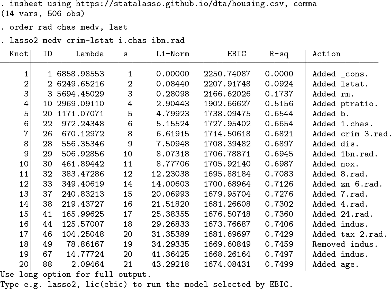
After importing the data and changing the variable order (to simplify the syntax), we use the lasso estimator by regressing the outcome variable (medv) against 11 continuous predictors (crim-lstat), the binary Charles River dummy variable chas, and the highway accessibility index rad, which we treat as categorical.

The lasso2 output above shows the following columns:

• Knot is the knot index. Knots are points at which predictors enter or leave the model. The default output shows one line per knot. If the long option is specified, one row per λ_r value is shown.

• ID shows the λ_r index, that is, r. By default, lasso2 uses a descending sequence of 100 penalty levels.

• s is the number of predictors in the model.

• L1-Norm shows the ℓ ₁ norm of coefficient estimates.

• The sixth column (here labeled EBIC) shows one out of four information criteria. The ic() option controls which information criterion is displayed, where string can be replaced with aic, aicc, bic, and ebic (the default).

• R-sq shows the R ² value.

• The final column shows which predictors are entered or removed from the model at each knot. The order in which predictors are entered into the model can be interpreted as an indication of the relative predictive power of each predictor.

Because lambda( real ) is not specified, lasso2 obtains the coefficient path for a default list of λ_r values. The largest penalty level is 6858.99, in which case the model does include only the constant.

We use the ibn. prefix for rad instead of the i. prefix commonly used in regression analysis. The i. prefix makes Stata omit the (automatically selected) base category from the estimation to avoid perfect collinearity (see help fvvarlist). In contrast with OLS, the lasso does not require the full-rank condition, allowing us to include one dummy for every category without removing the base category dummy. In this way, we let the lasso choose the base category automatically as the categories omitted from the selected model.

Figure 5 shows the coefficient path of the lasso for selected variables as a function of ln(λ). The graph illustrates how the lasso shrinks coefficients toward zero as the penalty level increases (from left to right). We can also infer the order in which predictors leave the model. The figure was created using the following command:

Figure 5.

The coefficient path of the lasso for selected variables as a function of ln(λ)

The plotpath() option passes settings to Stata’s line command and is used here to switch the legend off. Instead of a standard legend, we specify plotlabel to show variable names on the left-hand side of the graph.

The commands of lassopack support Stata’s factor-variable notation. This is especially useful when the relationship between the outcome variable and predictors is suspected to be nonlinear. For demonstration purposes, we add squared terms and interaction effects. We also allow the effect of lstat to depend on whether the binary Charles River dummy variable (chas) takes the values 1 or 0.

lasso2 supports model selection using information criteria. To this end, we use the replay syntax with the lic() option, which avoids fitting the full model again. The lic() option can also be specified in the first lasso2 call. In the following example, the replay syntax works similarly to a postestimation command:

Two columns are shown in the output: one for the lasso estimator and one for postestimation OLS, which applies OLS to the model selected by the lasso.

K-fold CV with cvlasso

Next, we consider K-fold CV:

The cvlasso output displays four columns: the index of λ_r (that is, r), the value of λ_r , the estimated mean squared prediction error, and the standard deviation of the MSPE. The output indicates the value of λ_r that corresponds to the lowest MSPE with an asterisk (*). We refer to this value as ${\widehat{\lambda }}_{\text{lopt}}$ . In addition, the symbol ⁁ marks the largest value of λ that is within one standard error of ${\widehat{\lambda }}_{\text{lopt}}$ , which we denote as ${\widehat{\lambda }}_{\text{lse}}$ .

The mean squared prediction is shown in figure 6, which was created using the plotcv option. The graph shows the mean squared prediction error estimated by CV along with ± one standard error. The continuous and dashed vertical lines correspond to ${\widehat{\lambda }}_{\text{lopt}}$ and ${\widehat{\lambda }}_{\text{lse}}$ , respectively.

Figure 6.

The MSPE estimated by CV along with ± one standard error. The continuous and dashed vertical lines correspond to lopt and lse, respectively.

To fit the model corresponding to either ${\widehat{\lambda }}_{\text{lopt}}$ or ${\widehat{\lambda }}_{\text{lse}}$ , we use the lopt or lse option, respectively. Similarly to the lic() option of lasso2, lopt and lse can be specified either in the first cvlasso call or after estimation using the replay syntax as in this example:

Rigorous penalization with rlasso

Lastly, we consider rlasso, which runs an iterative algorithm to estimate the penalty level and loadings. In contrast with lasso2 and cvlasso, it reports the selected model directly.

The supscore option prompts the sup-score test of joint significance. The p-value is obtained through multiplier bootstrap. The test statistic of 16.15 can also be compared with the asymptotic 5% critical value (here 3.75).

7.2 Time-series data

A standard problem in time-series econometrics is to select an appropriate lag length. In this subsection, we show how lassopack can be used for this purpose. We consider Stata’s built-in dataset lutkepohl2.dta, which includes quarterly (log-differenced) consumption (dln_consump), investment (dln_inv), and income (dln_inc) series for West Germany from quarter 1 1960–quarter 4 1982. We demonstrate both lag selection via information criteria and by h-step-ahead rolling CV. We do not consider the rigorous penalization approach of rlasso because of the assumption of independence, which seems too restrictive in the time-series context.

Information criteria

After importing the data, we run the most general model with up to 12 lags of the variables dln_consump, dln_inv, and dln_inc using lasso2 with the lic(aicc) option.

The output consists of two parts. The second part of the output is prompted because lic(aicc) is specified. lic(aicc) asks lasso2 to fit the model selected by AIC _c , which in this case corresponds to λ ₁₁ = 0.207.

h-step-ahead rolling CV

In the next step, we consider h-step-ahead rolling CV.

The output indicates how the dataset is partitioned into training data and the validation point. For example, the shorthand 13-80 (81) in the output above indicates that observations 13 to 80 constitute the training dataset in the first step of CV, and observation 81 is the validation point. The options fixedwindow, h(), and origin() can be used to control the partitioning of data into training and validation data. h() sets the parameter h. For example, h(2) prompts 2-step-ahead forecasts (the default is h(1)). fixedwindow ensures that the training dataset is the same size in each step. If origin(50) is specified, the first training partition includes observations 13 to 50, as shown in the next example:

The option plotcv creates the graph of the estimated mean squared prediction in figure 7. To fit the model corresponding to ${\widehat{\lambda }}_{\text{lse}}$ , we can—as in the previous examples—use the replay syntax:

Figure 7.

CV plot. The graph uses Stata’s built-in dataset lutkepohl2.dta and 1-stepahead rolling CV with origin(50).

Take care when setting the parameters of h-step-ahead rolling CV. The default settings have no particular econometric justification.

8 Monte Carlo simulation

We have introduced three alternative approaches for setting the penalization parameters in sections 3–5. In this section, we present the results of Monte Carlo simulations, which assess the performance of these approaches in terms of in-sample fit, out-of-sample prediction, model selection, and sparsity. To this end, we generate artificial data using the process

$y_i=1+{\displaystyle \sum _{j=1}^p{\beta }_j{x}_{ij}+{\epsilon }_i,\hspace{0.17em}\hspace{0.17em}\hspace{0.17em}{\epsilon }_i}\sim N\left(0,{\sigma }^2\right),\hspace{0.17em}\hspace{0.17em}\hspace{0.17em}i=1,\dots ,2n$

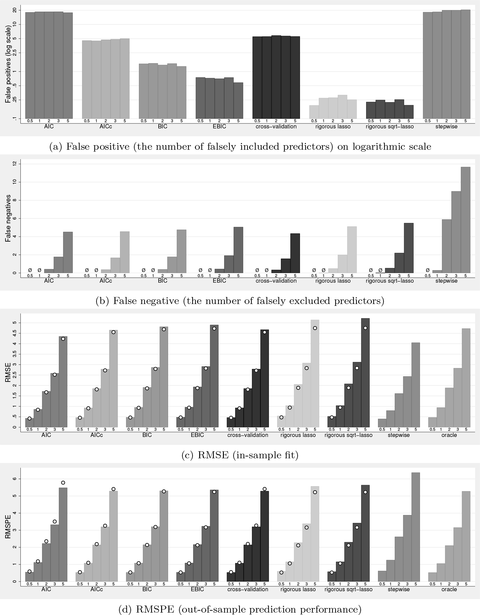
with n = 200. We report results for p = 100 and for the high-dimensional setting with p = 220. The predictors x_ij are drawn from a multivariate normal distribution with corr(x_ij, x_ir ) = 0.9^|j−r|. We vary the noise level σ between 0.5 and 5; specifically, we consider σ = {0.5, 1, 2, 3, 5}. We define the parameters as ${\beta }_j=\mathbb{1}\left\{j\le s\right\}$ for j = 1,…, p with s = 20, implying exact sparsity. This simple design allows us to gain insights into the model-selection performance in terms of false-positive frequency (the number of variables falsely included) and false-negative frequency (the number of variables falsely omitted) when relevant and irrelevant regressors are correlated. All simulations use at least 1,000 iterations. We report additional Monte Carlo results in appendix A.1, where we use a design in which coefficients alternate in sign.

Because the aim is to assess in-sample and out-of-sample performance, we generate 2n observations and use the data i = 1,…, n as the estimation sample and the observations i = n + 1,…, 2n for assessing out-of-sample prediction performance. This allows us to calculate the rmse and root mean squared prediction error (RMSPE) as

$\text{rmse}=\sqrt{\frac{1}{n}{\displaystyle \sum _{i=1}^n{\left(y_i-{\widehat{y}}_{i,n}\right)}^2}}\text{and}\text{RMSPE}=\sqrt{\frac{1}{n}{\displaystyle \sum _{i=n+1}^{2n}{\left(y_i-{\widehat{y}}_{i,n}\right)}^2}}$

9

where ${\widehat{y}}_{i,n}$ are the predictions from fitting the model to the first n observations.

Figures 8 and 9 illustrate results for the following estimation methods implemented in lassopack: the lasso with λ selected by AIC, BIC, EBIC _ξ , and AIC _c (as implemented in lasso2); the rigorous lasso and the rigorous square-root lasso (implemented in rlasso) using the X-independent penalty choice; and the five-fold cross-validated lasso using the penalty level that minimizes the estimated MSPE (implemented in cvlasso). In addition, we report postestimation OLS results (denoted by dots).

Figure 8.

Monte Carlo simulation for an exactly sparse parameter vector with p = 100 and n = 200

Figure 9.

Monte Carlo simulation for an exactly sparse parameter vector with p = 220 and n = 200

For comparison, we also show results of stepwise regression (for p = 100 only) and the oracle estimator. Stepwise regression starts from the full model and iteratively removes regressors if the p-value is above a predefined threshold (10% in our case). Stepwise regression is known to suffer from overfitting and pretesting bias. However, it still serves as a relevant reference point because of its connection with ad hoc model selection using hypothesis testing and the general-to-specific approach. The oracle estimator is OLS applied to the predictors included in the true model. Naturally, the oracle estimator is expected to show the best performance but is not feasible in practice because the true model is not known. The results of figures 8 and 9 are also reported in tabular form in tables 5 and 6 in appendix A.2 along with additional information, including results for the rigorous lasso and rigorous square-root lasso with an X-dependent penalty choice.

We first summarize the main results in figure 8 for the case where p = 100. AIC and stepwise regression exhibit the worst selection performance, with around 18–20 falsely included predictors on average. While AIC and stepwise regression achieve the lowest rmse (best in-sample fit), the out-of-sample prediction performance is among the worst—a typical symptom of overfitting. Note that in-sample fit of AIC and stepwise even exceed the fit of the oracle estimator. The corrected AIC improves upon the standard AIC in terms of both false-positive rate and prediction performance.

Compared with AIC _c , the BIC-type information criteria show similar out-of-sample prediction and better selection performance. While the EBIC performs only marginally better than BIC in terms of false positives, we expect the relative performance of BIC and EBIC to shift in favor of EBIC as p increases relative to n. Five-fold CV with the lasso behaves very similarly to the AIC _c across all measures. The rigorous lasso, rigorous square-root lasso, and EBIC exhibit overall the lowest false-positive rates, whereas rigorous methods yield slightly higher rmse and RMSPE than information criteria and CV-based methods.

Postestimation OLS generally exhibits better in-sample fit, indicating that the shrinkage bias from penalization can be alleviated by applying OLS to the selected model. In terms of out-of-sample prediction, postestimation OLS performs worse than first-step lasso when variable-selection performance is poor (particularly for the AIC) but leads to performance improvements for rigorous methods.

We also present simulation results for the high-dimensional setting in figure 9. Specifically, we consider p = 220 instead of p = 100, while keeping the estimation sample size constant at n = 200. With between 164 and 195 included predictors on average, the AIC suffers from overfitting. The RMSPE of the AIC exceeds the rmse by a factor of 5 or more. In comparison, aic _c and five-fold cv perform better as model selectors, with a false-positive frequency between six and eight predictors.

Despite many predictors to choose from, EBIC and rigorous methods perform generally well in recovering the true structure. The false-positive frequency is below 1 across all noise levels, and the false-negative rate is zero if σ is 1 or smaller. While the BIC performs similarly to the EBIC for σ = 0.5 and σ = 1, its performance resembles the poor performance of AIC for larger noise levels. The Monte Carlo results in table 6 in appendix A.2 highlight that EBIC and rigorous methods are well suited for the high-dimensional setting where p > n, while AIC and BIC are not appropriate.

The computational costs of each method are reported in table 3. rlasso with X-independent penalty is the fastest method considered. The runtimes of lasso and square-root lasso with p = 100 are 0.1s and 0.4s, respectively. The computational cost increased only slightly if p is increased to p = 220. rlasso with an X-dependent penalty simulates the distribution of the maximum value of the score vector. This process increases the computational cost of the rigorous lasso to 5.9 seconds for p = 100 (12.7 seconds for p = 220). With an average runtime of 3.1 seconds, lasso2 is slightly faster than rlasso with X-dependent penalty if p = 100 but slower in the high-dimensional setup. Unsurprisingly, K-fold CV is the slowest method because it requires the model to be fit K times for a range of tuning parameters.

Table 3.

Runtime with p = 100 and p = 220

Method	Call	Seconds p = 100	p = 220
Rigorous lasso	rlasso y x	0.09	0.24
with X-dependent penalty	rlasso y x, xdep	5.92	12.73
Rigorous square-root lasso	rlasso y x, sqrt	0.39	0.74
with X-dependent penalty	rlasso y x, sqrt xdep	3.34	7.03
CV	cvlasso y x, nfolds(5) lopt	23.50	293.93
Information criteria	lasso2 y x	3.06	44.06
Stepwise regression	stepwise, pr(.1): reg y x	4.65	–

note: PC specification: Intel Core i5-6500 with 16 GB RAM, Windows 7.

9 Technical notes

9.1 Pathwise coordinate-descent algorithms

lassopack implements the elastic net and square-root lasso using coordinate-descent algorithms. The algorithm—then referred to as “shooting”—was first proposed by Fu (1998) for the lasso and by Van der Kooij (2007) for the elastic net. Belloni, Chernozhukov, and Wang (2011, 2014) use the coordinate descent for the square-root lasso and have kindly provided MATLAB code.

Coordinate-descent algorithms repeatedly cycle over predictors j = 1,…, p and update single-coefficient estimates until convergence. Suppose the predictors are centered and standardized to have unit variance, and the penalty loadings are ψ_j = 1 for all j. In that case, the update for coefficient j is obtained using univariate regression of the current partial residuals (that is, excluding the contribution of predictor j) against predictor j. More precisely, the update for the elastic net is calculated as

${\tilde{\beta }}_j\leftarrow \frac{S\left\{{\displaystyle {\sum }_{i=1}^n{x}_{ij}\left(y_i-{\tilde{y}}_i^{\left(j\right)}\right),\lambda \alpha }\right\}}{1+\lambda \left(1-\alpha \right)}$

where ${\tilde{\beta }}_j$ denotes the current coefficient estimate and ${\tilde{y}}_i^{\left(j\right)}={\displaystyle {\sum }_{\mathcal{l}\ne j}{x}_{i\mathcal{l}}{\tilde{\beta }}_{\mathcal{l}}}$ is the predicted value without the contribution of predictor j. Thus, because the predictors are standardized, ${\displaystyle {\sum }_i{x}_{ij}\left(y_i-{\tilde{y}}_i^{\left(j\right)}\right)}$ is the OLS estimate of regressing predictor j against the partial residual $\left(y_i-{\tilde{y}}_i^{\left(j\right)}\right)$ . The function S(a, b), referred to as the soft-thresholding operator, is

$S(a,b)=\{\begin{array}{ll}a-b\hfill & \text{if }a>0\text{ and }b<|a|\hfill \\ a+b\hfill & \text{if }a<0\text{ and }b<|a|\hfill \\ 0\hfill & \text{if }b>|a|\hfill \end{array}$

and it sets some of the coefficients equal to zero. The coordinate-descent algorithm is spelled out for the square-root lasso in Belloni, Chernozhukov, and Wang (2014, supplementary material). ²⁵

The algorithm requires an initial beta estimate for which the ridge estimate is used. If the coefficient path is obtained for a list of λ values, lasso2 starts from the largest λ value and uses previous estimates as initial values (“warm starts”). See Friedman et al. (2007) and Friedman, Hastie, and Tibshirani (2010) and references therein for further information.

9.2 Standardization

Because penalized regression methods are not invariant to scale, it is common practice to standardize the regressors x_ij such that ${\displaystyle {\sum }_i{x}_{ij}^2=1}$ before computing the estimation results and then to unstandardize the coefficients after estimation. We refer to this approach as preestimation standardization. An alternative is to standardize on the fly by adapting the penalty loadings. The results are equivalent in theory. In the case of the lasso, setting ${\psi }_j={\left({\displaystyle {\sum }_i{x}_{ij}^2}\right)}^{1/2}$ yields the same results as dividing the data by ${\displaystyle {\sum }_i{x}_{ij}^2}$ before estimation. Standardization on the fly is the default in lassopack because it tends to be faster. Preestimation standardization can be used with the prestd option, which can lead to improved numerical precision or more stable results in the case of difficult problems; the cost is (a typically small) computation time required to standardize the data. The unitloadings option can be used if the researcher does not want to standardize data. If the preestimation-standardization and standardizationon-the-fly results differ, the user can compare the values of the penalized minimized objective function saved in e(pmse) (the penalized mean squared error for the elastic net) or e(prmse) (the penalized rmse for the square-root lasso).

9.3 Zero penalization and partialing out

In many applications, theory suggests that specific predictors affect the outcome variable. Hence, it might be desirable to always include these predictors in the model to improve finite-sample performance. Typical examples are the intercept, a time trend, or any other predictor that the researcher has prior knowledge of. lassopack offers two approaches for such situations:

• Zero penalization: The notpen() option of lasso2 and cvlasso allows one to set the penalty for specific predictors to 0; that is, ψ_ℓ = 0 for some ℓ ∊ {1,…, p}. Those variables are not subject to penalization and will always be included in the model. rlasso supports zero penalization through the pnotpen() option, which accommodates zero penalization in the rigorous-lasso penalty loadings; see below.

• • Partialing out: We can also apply the penalized regression method to the data after the effect of certain regressors has been partialed out. Partialing out is supported by lasso2, cvlasso, and rlasso using the partial() option. The penalized regression does not yield estimates of the partialed-out coefficients directly. Instead, lassopack recovers the partialed-out coefficients by postestimation OLS.

The two methods—zero penalization and partialing out—are numerically equivalent. Formally, suppose we do not want to subject predictors ℓ with $\overline{p}>\mathcal{l}\ge p$ to penalization. The zero-penalization and partialed-out lasso estimates are defined, respectively, as

$\begin{array}{ll}\hfill \widehat{\beta }\left(\lambda \right)& =\arg \min \frac{1}{n}{\displaystyle \sum _{i=1}^n{(y_i-{\displaystyle \sum _{j=1}^{\overline{p}}{x}_{ij}{\beta }_j-}{\displaystyle \sum _{\mathcal{l}=\overline{p}+1}^p{x}_{i\mathcal{l}}{\beta }_{\mathcal{l}}})}^2+\frac{\lambda }{n}}{\displaystyle \sum _{j=1}^{\overline{p}}{\psi }_{ij}|{\beta }_j|}\hfill \\ \hfill \text{and}\widehat{\beta }\left(\lambda \right)& =\arg \min \frac{1}{n}{\displaystyle \sum _{i=1}^n{\left({\tilde{y}}_i-{\displaystyle \sum _{j=1}^{\overline{p}}{\tilde{x}}_{ij}{\beta }_j}\right)}^2+\frac{\lambda }{n}}{\displaystyle \sum _{j=1}^{\overline{p}}{\psi }_j|{\beta }_j|}\hspace{0.17em}\hspace{0.17em}\hfill \end{array}$

where ${\tilde{y}}_i=y_i-{\displaystyle {\sum }_{\mathcal{l}=\overline{p}+1}^p{x}_{i\mathcal{l}}{\widehat{\delta }}_{y,\mathcal{l}}}$ and ${\tilde{x}}_{ij}=x_{ij}-{\displaystyle {\sum }_{\mathcal{l}=\overline{p}+1}^p{x}_{i\mathcal{l}}{\widehat{\delta }}_{j,\mathcal{l}}}$ are the residuals of regressing y and the penalized regressors against the set of unpenalized regressors. The equivalence states that ${\widehat{\beta }}_j={\tilde{\beta }}_j$ for all $j=1,\text{…},\overline{p}$ . The result is spelled out in Yamada (2017) for the lasso and ridge but holds for the elastic net more generally.

The partial() or notpen() option can be used for variables that should not be penalized by the lasso. The options are equivalent in theory (see above), but their numerical results can differ in practice because of the different calculation methods used. Partialing out variables can lead to improved numerical precision or more stable results in the case of difficult problems compared with zero penalization but may be slower in terms of computation time.

The estimation of penalty loadings in the rigorous lasso introduces an additional complication that necessitates the rlasso-specific option pnotpen(). The theory for the rlasso penalty loadings is based on the penalized regressors after partialing out the unpenalized variables. The pnotpen() option guarantees that the penalty loadings for the penalized regressors are the same as if the unpenalized regressors had instead first been partialed out.

The fe (fixed-effects) option is equivalent to (but computationally faster and more accurate than) specifying unpenalized panel-specific dummies. The fixed-effects (within) transformation also removes the constant and the fixed effects. The panel variable used by the fe option is the panel variable set by xtset. If installed, the within transformation uses the fast ftools package by Correia (2016).

The prestd, notpen(), and pnotpen() options can be used as simple checks for numerical stability by comparing results that should be equivalent in theory. The values of the penalized minimized objective function saved in e(pmse) for the elastic net and e(prmse) for the square-root lasso may also be used for comparison.

9.4 Treatment of the constant

By default, the constant (if present) is not penalized; this is equivalent to mean centering prior to estimation. The partial() option also partials out the constant (if present). To partial out the constant only, we can specify partial(_cons). Both partial() and fe mean-center the data; the noconstant option is redundant in this case and may not be specified with these options. If the noconstant option is specified, an intercept is not included in the model, but the estimated penalty loadings are still estimated using mean-centered regressors (see the center option).

11 Programs and supplemental materials

Supplemental Material, st0594 - lassopack: Model selection and prediction with regularized regression in Stata

Supplemental Material, st0594 for lassopack: Model selection and prediction with regularized regression in Stata by Achim Ahrens, Christian B. Hansen and Mark E. Schaffer in The Stata Journal