Conducting sensitivity analysis for unmeasured confounding in observational studies using E-values: The evalue package

Abstract

In this article, we introduce the evalue package, which performs sensitivity analyses for unmeasured confounding in observational studies using the methodology proposed by VanderWeele and Ding (2017, Annals of Internal Medicine 167: 268–274). evalue reports E-values, defined as the minimum strength of association on the risk-ratio scale that an unmeasured confounder would need to have with both the treatment assignment and the outcome to fully explain away a specific treatment-outcome association, conditional on the measured covariates. evalue computes E-values for point estimates (and optionally, confidence limits) for several common outcome types, including risk and rate ratios, odds ratios with common or rare outcomes, hazard ratios with common or rare outcomes, standardized mean differences in outcomes, and risk differences.

1 Introduction

A fundamental concern when conducting evaluations using observational data is that unmeasured confounding—one or more additional factors that cause both the treatment assignment and the outcome—might be mistaken for a treatment effect. For this reason, researchers endeavor to adjust for all variables considered to influence these associations when performing analyses. However, in observational research, it is unlikely that data for all potential confounding variables will be available. Thus, one should conduct a postestimation sensitivity analysis to assess how strong a relationship would have to be between an unmeasured confounder and the treatment assignment, as well as between the unmeasured confounder and the outcome, to explain away an observed treatment effect.

Several sensitivity analyses have been developed for different statistical models (see, for example, Cornfield et al. [1959]; Rosenbaum and Rubin [1983]; Manski [1990]; Lin, Psaty, and Kronmal [1998]; Rosenbaum [2002, 2010]; Brumback et al. [2004]; Vander-Weele and Arah [2011]; Imbens [2003]; Imbens and Rubin [2015]; Ding and VanderWeele [2016]; and VanderWeele and Ding [2017]). Four community-contributed packages are currently available for conducting sensitivity analysis in Stata: rbounds (Gangl 2004), mhbounds (Becker and Caliendo 2007), sensatt (Nannicini 2007), and episens (Orsini et al. 2008). The first three commands are designed for use with matching estimators based on the approaches developed by Rosenbaum and Rubin (1983) and Rosenbaum (2002), and the fourth uses the methods described by Greenland (1996) for assessing sensitivity in epidemiology (2 × 2) tables.

In this article, we introduce the evalue package, which performs sensitivity analyses for unmeasured confounding in observational studies using the methodology proposed by VanderWeele and Ding (2017). evalue reports the E-value, which is defined as the minimum strength of association, on the risk-ratio (RR) scale that an unmeasured confounder would need to have with both the treatment assignment and the outcome, conditional on the measured covariates, to explain away a treatment-outcome association. In contrast with most other sensitivity analysis approaches that focus on whether confounding of a specified strength would suffice to explain away an effect estimate, the E-value focuses on the magnitude of the confounder associations that could produce confounding bias equal to the observed treatment-outcome association. The E-value approach and formulas are applicable for multiple confounders. The magnitude of the confounding associations is then interpreted as the maximum RRs that could be produced comparing any two values of the whole set of unmeasured confounders (conditional on the measured covariates). See VanderWeele, Ding, and Mathur (2019) for further discussion and examples. The investigator does not choose the confounding variables (or specify their confounding associations) but merely reports how strongly an unmeasured confounder must be related to the treatment assignment and outcome to explain away an effect estimate; readers or other researchers may then assess whether the confounder associations of that magnitude are plausible.

2 Methods

The E-value is computed on the RR scale, so results of statistical models other than the RR must be converted to the RR scale. In this section, we present the methods involved in computing the E-value for various model types.

2.1 E-value for RR and rate ratio

The basic formula for computing an E-value for any outcome type on the RR scale (and its confidence limit closest to the null) is as follows (VanderWeele and Ding 2017): ¹

If RR > 1:

E-value (point estimate) $=\text{RR}+\sqrt{\text{RR}\times (\text{RR}-1)}$

E-value (lower limit [LL]) = 1 if LL ≤ 1, else $\text{LL}+\sqrt{\text{LL}\times (\text{LL}-1)}$

If RR < 1:

E-value (point estimate) $=\text{ 1}/\text{RR}+\sqrt{1/\text{RR}\times (1/\text{RR}-1)}$

E-value (upper limit [UL]) = 1 if UL ≥ 1, else $1/\text{UL}+\sqrt{1/\text{UL}\times (1/\text{UL}-1)}$

2.2 E-value for odds ratio

When the outcome is relatively rare (for example, < 15% prevalence by the end of follow-up), the odds ratio (OR) approximates the RR, so the basic E-value formula (in section 2.1) should be used. In a case–control study, the outcome needs to be rare only in the underlying population, not in the study sample (the same considerations hold when the outcome prevalence is instead approximately > 85% by the end of follow-up because the variable coding can simply be reversed). When the outcome is not rare (between 15% and 85% prevalence at the end of follow-up), an approximate E-value may be obtained by replacing the RR with the square root of the OR (VanderWeele 2017); that is, $\text{RR}\approx \sqrt{\text{OR}}$ in the E-value formula presented in section 2.1. Note that when the outcome is rare, the $\sqrt{\text{OR}}$ transformation provides a poor approximation, so the calculations under the “rare” outcome assumption should be used. However, when the probability of the outcome is between 15% and 85%, the $\sqrt{\text{OR}}$ approximation works quite well (Ding and VanderWeele 2016).

2.3 E-value for hazard ratio

When the outcome is relatively rare as described above, the basic E-value formula (in section 2.1) should be used. When the outcome is common, an approximate E-value may be obtained (VanderWeele 2017) by applying the approximation $\text{RR}\approx \left(1-0.{\text{5}}^{\sqrt{\text{HR}}}\right)/\left(1-0.{\text{5}}^{\sqrt{1/\text{HR}}}\right)$ in the E-value formula in section 2.1.

2.4 E-value for standardized mean difference

With standardized effect sizes d (mean of the outcome variable divided by the pooled standard deviation [SD] of the outcome) and a standard error for this standardized effect size SD, an approximate E-value may be obtained (Lipsey and Wilson 2001; Vander-Weele 2017; Linden 2019) by applying the approximation RR ≈ e ^{[0 . 91 × d ]} in the E-value formula. Similarly, an approximate confidence interval (CI) for the RR may be obtained by using the approximation (e ^{[0 . 91 × d − 1 . 78 × SD]}, e ^{[0 . 91 × d +1 . 78 × SD]}). This approach relies on additional assumptions and approximations. Other sensitivity analysis techniques have been developed for this setting (Lin, Psaty, and Kronmal 1998; Imbens 2003; VanderWeele and Arah 2011), but they generally require additional assumptions, and the variables do not necessarily have a corresponding E-value.

2.5 E-value for risk difference

If the adjusted risks for the treated and untreated are p ₁ and p ₀, then the E-value may be obtained by replacing the RR with p ₁ /p ₀ in the E-value formula. The E-value for the CI on a risk-difference (RD) scale is complex, requiring the computation of several measures and then the use of a grid search to find the corresponding bias factor that, when transformed to the RR scale, will elicit the E-value of the lower confidence limit (see Ding and VanderWeele [2016] for a comprehensive discussion). Alternatively, if the outcome probabilities p ₁ and p ₀ are not small or large (for example, if they are between 0.20 and 0.80), then the approximate approach for differences in continuous outcomes given in section 2.4 may be used. Other sensitivity analysis techniques have been developed for this setting (Lin, Psaty, and Kronmal 1998; Imbens 2003; VanderWeele and Arah 2011) but generally require additional assumptions and do not provide a corresponding E-value.

2.6 E-values for nonnull hypotheses

Thus far, we have described how to calculate E-values to assess the minimum strength of the association an unmeasured confounder would need to have with both the treatment assignment and the outcome to move the point estimate, or one limit of the CI, to the null. However, a similar procedure can be used to assess the minimum magnitude of both confounder associations that would be needed to move an estimate to some other value of the RR. If we have an observed RR of RR and want to assess the minimum strength of both associations that would be needed to shift the estimate to some other value RR ^T , then we first take the ratio of the two values, RR/RR ^T , and then apply the E-value formula presented in section 2.1 to this ratio. We encourage investigators to read the original article introducing the E-value (VanderWeele and Ding 2017) to aid in understanding and interpretation prior to using the package.

3 The evalue package

This section describes the syntax of the commands in the evalue package for various model types.

3.1 Syntax

E-value for RR and rate ratio:

evalue rr point_estimate [ , lcl(# ) ucl( # ) true( # )

figure [( twoway_options )]]

E-value for OR:

evalue or point_estimate [, lcl( # ) ucl( # ) true( # ) common

figure [( twoway_options )]]

E-value for hazard ratio (HR):

evalue hr point_estimate [, lcl( # ) ucl( # ) true( # ) common

figure [( twoway_options )]]

E-value for standardized mean difference (SMD):

evalue smd point_estimate [, se( # ) true( # )

figure [( twoway_options )]]

E-value for RD:

evalue rd #a #b #c #d [, true( # ) level( # ) grid( # )

figure [( twoway_options )]]

In the syntax for evalue rd, #a is the number of exposed, diseased individuals (E = 1, D = 1); #b is the number of exposed, nondiseased individuals (E = 1, D = 0); #c is the number of unexposed, diseased individuals (E = 0, D = 1); and #d is the number of unexposed, nondiseased individuals (E = 0, D = 0). If the observed RD is negative, the exposure coding should first be reversed to yield a positive RD.

3.2 Options

lcl( # ) specifies the lower limit of the CI around the point estimate. evalue will use lcl() to compute an E-value for the CI limit if it is closer to the null than ucl(). This option is available for RR, OR, and HR models.

ucl( # ) specifies the upper limit of the CI around the point estimate. evalue will use ucl() to compute an E-value for the CI limit if it is closer to the null than lcl(). This option is available for RR, OR, and HR models.

se( # ) specifies the standard error of the point estimate of the SMD (for example, Cohen’s d) (see [R] esize). evalue will use se() to compute an E-value for the CI limit closest to the null. This option is available for SMD model.

true( # ) specifies a treatment-effects value to which to shift the observed point estimate other than the null effect. A null true effect (default values in evalue) is 0 in RD and SMD models and 1 in all ratio-type models.

common specifies that the outcome prevalence is between 15% and 85% at the end of follow-up for OR and HR models. When the common option is specified, an approximate E-value is obtained by replacing the RR with the square root of the OR (VanderWeele 2017). Note that when the outcome is rare, the $\sqrt{\text{OR}}$ transformation provides a poor approximation, and thus the calculations under the “rare” outcome assumption should be used (by not specifying common). However, when the prevalence of the outcome is between 15% and 85%, the $\sqrt{\text{OR}}$ approximation works quite well (Ding and VanderWeele 2016).

level( # ) specifies the confidence level, as a percentage, for the CI used for producing RD estimates. The default is level(95).

grid( # ) specifies the tolerance for the grid search of the E-value for an RD estimate. The default is grid(0.0001).

figure ( twoway_options ) produces a curve depicting the range of joint relationships (exposure–confounder and exposure–disease) that may explain away the estimated effect (and CI when applicable), with the computed E-values highlighted. A curve for the E-value of the CI is also displayed in the figure under the following conditions: 1) for RR, OR, and HR models, the user must specify lcl( # ) when the point estimate is greater than 1.0 or ucl( # ) when the estimate is lower than 1.0; 2) for an SMD model, the user must specify se( # ); 3) for an RD model, a CI curve is always produced; and 4) the computed E-value for the CI does not equal 1. Specifying figure without options uses the default graph settings.

4 Examples

evalue is designed similarly to an immediate command (see [U] 19 Immediate commands) in that it obtains point estimates and CI typed as arguments, rather than from data stored in memory. This allows an investigator to conduct sensitivity analyses on results published in the literature (which typically include only a point estimate and CI) and as a postestimation command using individual-level data. In the following examples, we illustrate both scenarios.

4.1 E-value for a RR

In a population-based case–control study, Victora et al. (1987) examined associations between breastfeeding and infant death by respiratory infection. After adjusting for age, birthweight, social status, maternal education, and family income, the authors found that infants fed only with formula were 3.9 (95% CI, 1.8 to 8.7) times more likely to die of respiratory infections than those who were exclusively breastfed. The investigators controlled for markers of socioeconomic status but not for smoking, and smoking may reduce breastfeeding and increase risk for respiratory death.

To compute the E-value for this relative risk, we type in the point estimate (3.9) and the lower and upper confidence limits (1.8 and 8.7, respectively). We also apply the figure option.

As shown in the output and figure, the E-value for the point estimate is 7.26. This E-value can be interpreted as follows: “The observed risk ratio of 3.9 could be explained away by an unmeasured confounder that was associated with both the treatment and the outcome by a risk ratio of 7.2-fold each, above and beyond the measured confounders, but weaker confounding could not do so” (VanderWeele and Ding 2017). Similarly, the E-value for the lower confidence limit (that is, the confidence limit closest to the null) is 3.0, which can be interpreted as “[a]n unmeasured confounder associated with respiratory death and breastfeeding by a risk ratio of 3.0-fold each could explain away the lower confidence limit, but weaker confounding could not” (VanderWeele and Ding 2017). The evidence for causality from these E-values thus looks reasonably strong because substantial unmeasured confounding would be needed to reduce the observed association or its CI to null (VanderWeele and Ding 2017).

4.2 E-value for an OR

In this example, we perform sensitivity analysis for a rare outcome rate (that is, < 15% of cases) by not specifying the common option. We use estimates from a study by Moorman et al. (2008) that indicated that in premenopausal women who breastfed for 6 to 12 months, the odds of developing ovarian cancer were 0.5 (95% CI: [0.3, 0.8]) times lower than in women who did not breastfeed.

As shown, the E-value for the point estimate is 3.41 and 1.81 for the CI. The point estimate seems moderately robust, but confounder associations with breastfeeding and ovarian cancer of this magnitude could potentially move the CI to the null.

4.3 E-value for a HR

In this example, we use the official Stata command stcox (see [ST] stcox) to estimate an HR and a CI using Cox regression and then pass on these estimates to evalue hr. The data are supplied with stcox and are for 48 participants in a cancer drug trial during which 64.6% of the patients died (a common outcome). Of these 48, 28 received treatment and 20 received a placebo. The participants ranged in age from 47 to 67 years. We fit a model to assess treatment effects, adjusting for patient age.

We see from the stcox output that the drug results in a much lower hazard (HR = 0.105; 95% CI: [0.04, 0.26])—and therefore a longer survivor time—than for those on the placebo (P < 0.001). The E-value for the HR is 8.25 and 4.48 for the upper confidence limit, suggesting that the evidence for causality is reasonably strong even when considering that existing confounding control was relatively poor.

4.4 E-value for a SMD

In this example, we illustrate how to convert a treatment-effects estimate derived from a linear regression model fit with a binary exposure to an SMD and how to then pass that estimate (and its standard error) to evalue smd. We begin by implementing regress (see [R] regress) to evaluate the effect of a mother’s smoking status during pregnancy on infant birthweight, using a subset of data by Cattaneo (2010). As covariates, we use mother’s age, education level, marital status, and whether this baby was the mother’s first birth.

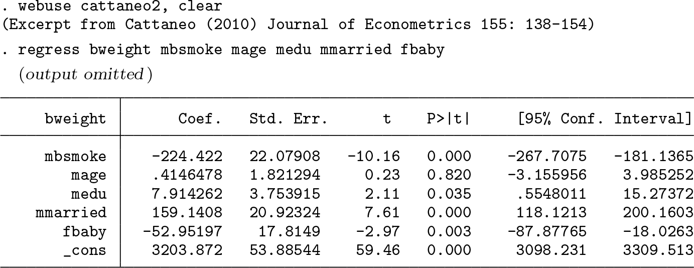
We see that the average birthweight of babies born to mothers who smoked is 224 grams less than babies whose mothers had not smoked. To convert this point estimate into an SMD, we implement the community-contributed command esizeregi (Linden 2019). To compute the SMD, we also need to retrieve the SD of the dependent variable (bweight) and get the number of observations in each group (mbsmoke).

Next, we plug the estimate and standard error into evalue smd to compute the E-values.

4.5 E-value for an RD

In this example, we illustrate how to compute the E-value for an RD of a binary outcome. Unlike the other evalue subcommands, where the user types in the point estimate and CI postmodel estimation, users of evalue rd enter the four values as they would for a 2 × 2 table (see epitab cs and csi), where #a is the number of exposed, diseased individuals (E = 1, D = 1); #b is the number of exposed, nondiseased individuals (E = 1, D = 0); #c is the number of unexposed, diseased individuals (E = 0, D = 1); and #d is the number of unexposed, nondiseased individuals (E = 0, D = 0).

Hammond and Horn (1958a,b) report associations between smoking and lung cancer deaths from a cohort study of 187,783 men, of which 42% were classified as having a history of regular cigarette smoking (exposed) versus others (no smoking or only occasional smoking). We could compute the RD and CI using csi, which gives us the RD estimate and CI of 0.00456 (95% CI: [0.00405, 0.00507]).

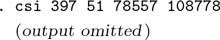
Using evalue rd, we enter these data as follows to compute the E-value:

These results can be interpreted as follows: “With an observed risk difference of RD = 0.00456, an unmeasured confounder that was associated with both regular smoking and lung cancer death by a risk ratio of 20.95-fold each, above and beyond the measured confounders, could explain away the estimate, but weaker confounding could not; to move the CI to include the null, an unmeasured confounder that was associated with both regular smoking and lung cancer death by a risk ratio of 15.96-fold each could do so, but weaker confounding could not” (VanderWeele and Ding 2017).

4.6 E-values for nonnull hypotheses

To this point, we described how to calculate E-values to assess the minimum strength of the association an unmeasured confounder would need to have with both the treatment and the outcome to move the point estimate, or one limit of the CI, to the null. However, we can use a similar procedure to assess the minimum magnitude of both confounder associations that would be needed to move an estimate to some other value of the RR. In evalue, we do this by specifying a desired value in the true() option.

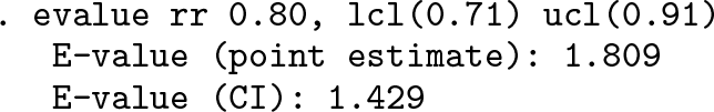
As an example, a study by the Agency for Healthcare Research and Quality (Ip et al. 2007) reported an RR between breastfeeding and childhood leukemia as 0.80 (95% CI: [0.71, 0.91]). Computing E-values for the null effect gives us 1.81 and 1.43 for the point estimate and CI, respectively.

Assume that we were interested in assessing how large both unmeasured confounding associations would need to be to shift the RR estimate from 0.80 to 0.90. We simply specify true(0.90).

As shown, we obtain an E-value for the point estimate of 1.50, which describes the magnitude of the associations an unmeasured confounder would need to have with breastfeeding and childhood leukemia to move the observed RR from 0.80 to 0.90. The interpretation of this nonnull E-value is that “for an unmeasured confounder to shift the observed estimate of RR = 0.80 to an estimate of RR ^T = 0.90, an unmeasured confounder that was associated with both breastfeeding and childhood leukemia by a risk ratio of 1.5-fold each could do so, but weaker confounding could not” (VanderWeele and Ding 2017). Because the CI already includes the value of 0.90, no additional unmeasured confounding is needed for the interval to include that value, and thus the E-value for the CI to include 0.90 is just E-value = 1.0.

We may also calculate E-values for the values of the RR on the other side of the null hypothesis. Thus, if we wanted to assess the minimum strength of both confounder associations that would be needed to move the RR estimate of 0.80 to an RR estimate of 1.20, we would simply specify true(1.20).

As shown, to shift estimates to an RR of 1.20, we obtain an E-value of 2.37 for the point and an E-value of 1.97 for the upper limit of the CI. The interpretation of these nonnull E-values would then be that for an unmeasured confounder to shift the observed RR estimate of 0.80 to an RR of 1.20, an unmeasured confounder that was associated with both breastfeeding and childhood leukemia by an RR of 2.37-fold each could do so, but a weaker confounder could not. Similarly, to shift the upper confidence limit of 0.91 to 1.20, an unmeasured confounder that was associated with both breastfeeding and leukemia by an RR of 1.97-fold each could do so, but a weaker confounder could not (VanderWeele and Ding 2017).

5 Discussion

In this article, we introduced the evalue package, which performs sensitivity analyses for unmeasured confounding in observational studies using the methodology proposed by VanderWeele and Ding (2017). A key advantage of this approach over other methods is its ease of use following common treatment-effects analyses. Investigators fit their adjusted models in the usual manner (for example, regression with covariates) and then simply apply evalue to the coefficient for the treatment variable and its CI. Similarly, evalue can readily compute E-values for treatment-effects estimates typically reported in published studies, thereby allowing readers to assess whether the confounder associations of that magnitude are plausible.

In conclusion, we have provided a convenient package for conducting sensitivity analysis following treatment-effects estimation in observational studies. We advocate the reporting of E-values in such studies to assist investigators and others in weighing the evidence for robustness to confounding and thus ultimately for causality.