Recommendations about estimating errors-in-variables regression in Stata

Abstract

Errors-in-variables (EIV) regression is a standard method for consistent estimation in linear models with error-prone covariates. The Stata commands eivreg and sem both can be used to compute the same EIV estimator of the regression coefficients. However, the commands do not use the same methods to estimate the standard errors of the estimated regression coefficients. In this article, we use analysis and simulation to demonstrate that standard errors reported by eivreg are negatively biased under assumptions typically made in latent-variable modeling, leading to confidence interval coverage that is below the nominal level. Thus, sem alone or eivreg augmented with bootstrapped standard errors should be preferred to eivreg alone in most practical applications of EIV regression.

1 Background

A common problem in many applied fields is estimating the coefficients of a linear regression model in which one or more of the independent variables is not observed directly but rather is measured with error. For example, in a traditional education production function model that may be used to estimate the effects of an educational policy on student achievement, current achievement is a function of the inputs of interest and prior achievement (Todd and Wolpin 2003). However, prior achievement is not observed; rather, it is measured with error by test scores (Lord 1980), often obtained from standardized assessments given by states or school districts in the United States. Fitting the model with error-prone measures used in place of their corresponding latent variables generally will yield inconsistent estimators of all model parameters, not just the regression coefficients corresponding to the variables measured with error (Buonaccorsi 2010; Carroll et al. 2006; Fuller 1987). This can lead, for example, to inconsistent estimators of treatment effects in analysis of covariance models where nonexperimental treatment groups have unequal distributions of confounders that are measured with error (Culpepper and Aguinis 2011; Lockwood and McCaffrey 2014).

Two primary methods are commonly used to obtain consistent estimators in settings where information about the magnitude of the measurement errors is known. The first, often referred to as errors-in-variables (EIV) regression, uses method-of-moments adjustment to account for the errors in measurement (Fuller 1987). This approach is implemented in the Stata command eivreg. The second common estimation method is via path analysis or structural equation models (for example, Bollen [1989]). This method commonly specifies a joint Gaussian distribution for the dependent and independent variables in the regression model and the measurement errors and then uses maximum likelihood to estimate the regression coefficients. This approach is implemented in the Stata command sem.

It can be shown that these two estimation approaches yield identical point estimates of regression coefficients, given the same data and same working values of the measurement error variances (see, for example, Buonaccorsi [2010, 115]). However, despite yielding common estimates of regression coefficients, eivreg and sem do not use the same methods to estimate the standard errors of the estimated regression coefficients. In this article, we use analysis and simulation to demonstrate that eivreg standard-error estimators are negatively biased under assumptions typically made in latent-variable modeling, leading to confidence interval coverage that is below the nominal level. Thus, sem alone or eivreg augmented with bootstrapped standard errors should be preferred to eivreg alone in most practical applications of EIV regression.

2 EIV regression

In this section, we first summarize the standard model assumptions for EIV regression, and we then define the EIV regression estimator. We then discuss differences in how eivreg and sem estimate standard errors for the estimated regression coefficients.

2.1 Model assumptions

We roughly follow the notation used in the Stata manual [R] eivreg. ¹ For i = 1,…, N, let $(Y_i,X_i^{\ast },X_i,U_i,\hspace{0.17em}{ϵ}_i)$ be independent and identically distributed (IID) from a distribution with finite fourth moments. The quantities $X_i^{\ast }$ , X _i , and U _i are each vectors of length p, so $X_i^{\ast } = (X_{i1}^{\ast }, . . . , X_{ip}^{\ast })\text{'}$ , X i = (X_{i 1} ,…, X_ip )′, and U _i = (U_{i 1} ,…, U^ip )′. The random variables Y_i and ϵ_i are scalars. The observed data are ${\{Y_i,X_i\}}_{i=1}^N$ , whereas ${\{X_i^{*},\hspace{0.17em}{U}_i,\hspace{0.17em}{ϵ}_i\}}_{i=1}^N$ are unobserved. The model assumptions are

$Y_i=X_i^{\ast }\prime \beta +{ϵ}_i,\hspace{0.17em}\hspace{0.17em}\hspace{0.17em}\hspace{0.17em}\hspace{0.17em}\hspace{0.17em}\hspace{0.17em}\hspace{0.17em}E({ϵ}_i|X_i^{\ast },U_i) = 0,\hspace{0.17em}\hspace{0.17em}\hspace{0.17em}\hspace{0.17em}\hspace{0.17em}\hspace{0.17em}\hspace{0.17em}\hspace{0.17em}\text{Var}({ϵ}_i) ={\sigma }^2\hspace{0.17em}\hspace{0.17em}\hspace{0.17em}\hspace{0.17em}\hspace{0.17em}\hspace{0.17em}\hspace{0.17em}\hspace{0.17em}\hspace{0.17em}\hspace{0.17em}\hspace{0.17em}\hspace{0.17em}\hspace{0.17em}\hspace{0.17em}\hspace{0.17em}\hspace{0.17em}\hspace{0.17em}\hspace{0.17em}\hspace{0.17em}\hspace{0.17em}$

1

$X_i=X_i^{\ast }+U_i,\hspace{0.17em}\hspace{0.17em}\hspace{0.17em}\hspace{0.17em}\hspace{0.17em}\hspace{0.17em}\hspace{0.17em}\hspace{0.17em}E(U_i|X_i^{\ast }, {ϵ}_i) =0,\hspace{0.17em}\hspace{0.17em}\hspace{0.17em}\hspace{0.17em}\hspace{0.17em}\hspace{0.17em}\hspace{0.17em}\hspace{0.17em}\text{Var}(U_i) ={\Sigma }_U\hspace{0.17em}\hspace{0.17em}\hspace{0.17em}\hspace{0.17em}\hspace{0.17em}\hspace{0.17em}\hspace{0.17em}\hspace{0.17em}\hspace{0.17em}\hspace{0.17em}\hspace{0.17em}\hspace{0.17em}\hspace{0.17em}\hspace{0.17em}\hspace{0.17em}\hspace{0.17em}\hspace{0.17em}\hspace{0.17em}$

2

Thus, the outcome of interest Y_i depends on the latent covariates $X_i^{\ast }$ through the linear regression in (1) with coefficients β and residual variance σ ². We refer to this regression model as the “true” regression model, and the goal is consistent estimation of β from this model. The challenge is that $X_i^{\ast }$ is measured with error by X _i . As noted in (2), the measurement errors U _i are assumed to have mean zero and positive semidefinite variance–covariance matrix Σ _U . Some of the components of $X_i^{\ast }$ may be measured without error by the corresponding components of X _i , in which case the corresponding components of U _i are identically zero and the corresponding elements of Σ _U are zero. Thus, X _i may generally contain both error-free and error-prone covariates, including a column of ones corresponding to an intercept.

Ignoring the fact that X _i measures $X_i^{\ast }$ with error by using ordinary least squares (OLS) in a regression of Y_i on X _i generally yields inconsistent estimates of β(Buonaccorsi 2010; Carroll et al. 2006; Fuller 1987). For example, consider the simple case where $X_i^{\ast }$ = (1, $X_i^{\ast }$ )′ for a scalar latent predictor $X_i^{\ast }$ measured with error by X_i and where the coefficient on $X_i^{\ast }$ in the true regression is β. Then, the estimated coefficient on X_i from a regression of Y_i on X _i = (1, X_i )′ converges in probability to rβ, where r is the “reliability” of X_i as a measure of $X_i^{\ast }$ , equal to the ratio of the variance of $X_i^{\ast }$ to the variance of X_i . Because 0 < r ≤ 1, the estimated coefficient is said to be “attenuated” because it converges to a value closer to zero than the true coefficient β. In more complex problems, the directions and magnitudes of the asymptotic bias in estimators of β will depend on the true coefficients and the distribution of both $X_i^{\ast }$ and U _i .

2.2 The EIV regression estimator

The EIV regression estimator uses method of moments to estimate β, provided that the variance–covariance matrix of the measurement errors Σ _U is known or can be estimated. Under the model assumptions in (1) and (2), the EIV regression estimator of β is consistent, provided other standard regularity conditions hold. In this section, we summarize the EIV regression estimator.

We restrict attention to the case in which Σ _U is a diagonal matrix with elements (σ_U ² ₁ ,…, σ_U ² _p ), so the measurement errors in different components of X _i are mutually uncorrelated. We focus on this case because this assumption is commonly made in applications and because this restriction is required by eivreg. The EIV regression estimator is still well defined in cases where Σ _U is not diagonal (Fuller 1987), and in such cases, Stata users could use sem rather than eivreg because the syntax for sem is sufficiently general to allow nondiagonal specifications for Σ _U .

We further restrict attention to the case in which the measurement error variances $({\sigma }_{U1}^2, . . . , {\sigma }_{Up}^2)$ are not known, but rather the reliability of each component of X _i is known (or treated as known). For each component j = 1,…, p, the reliability is

$r_j=\frac{\text{Var}\left(X_{ij}^{\ast }\right)}{\text{Var}\left(X_{ij}\right)}= \frac{\text{Var}\left(X_{ij}^{\ast }\right)}{\text{Var}\left(X_{ij}^{\ast }\right) +{\sigma }_{Uj}^2}$

We focus on this case because, again, it is common in applications and because if $({\sigma }_{U1}^2, . . . , {\sigma }_{Up}^2)$ were known, Stata users would be likely to use sem rather than eivreg because sem allows users to specify measurement error variances, whereas eivreg requires users to specify reliabilities. ² Note that 0 < r_j ≤ 1 as long as $\text{Var}\left(X_{ij}^{\ast }\right)>0$ , and r_j = 1 for any component j of $X_i^{\ast }$ that is measured without error. We assume ${\sigma }_{Uj}^2= 0$ if $\text{Var}\left(X_{ij}^{\ast }\right)=0$ (for example, the model intercept) and define r_j = 1 in that case.

Under the assumptions that Σ _U is diagonal and that the reliabilities (r ₁ ,…, r_p ) are treated as known, the EIV regression estimator first defines a working value ${\tilde{\Sigma }}_U$ of Σ _U . The matrix ${\tilde{\Sigma }}_U$ is set equal to a diagonal matrix with diagonal element j equal to $(1-r_j)\widehat{\text{Var}}(X_{ij})$ , where $\widehat{\text{Var}}(X_{ij}) = (1/N){\displaystyle {\sum }_{i=1}^N{(X_{ij}-{\overline{X}}_{·j})}^2}$ . The quantity $(1-r_j)\widehat{\text{Var}}(X_{ij})$ is the maximum likelihood estimator (MLE) of the measurement error variance ${\sigma }_{Uj}^2$ under the assumptions that r_j is known and that $(X_{ij}^{*}, U_{ij})$ have a bivariate normal distribution and is a consistent estimator of σ_U ² _j under weaker distributional assumptions.

Let Y = (Y ₁ ,…, Y_N )′, let X be the (N × p) matrix with row i equal to $X_i^{\prime }$ , let X ^∗ be the (N × p) matrix with row i equal to $X_i^{\ast }\prime$ , and define $S=N{\tilde{\Sigma }}_U$ . Then, the EIV regression estimator of β is

$b= {(X\prime X-S)}^{-1}X\prime Y=A^{-1}X\prime Y$

3

where A = X ′ X − S, as defined in the Stata manual [R] eivreg. The intuition for the estimator is that under the assumptions to this point, the diagonal elements of X ′ X are inflated relative to the corresponding diagonal elements of X ^∗′ X ^∗ because of the measurement errors, and subtraction of S corrects for this inflation in expectation. Under standard regularity conditions, $\text{plim}\{(1/N){(X\prime X-S)}^{-1}\}=E{(X_i^{\ast }{X}_i^{\ast }\prime )}^{-1}$ and $\text{plim}\{(1/N)X\prime Y\}=E(X_i^{\ast }{Y}_i) =E(X_i^{\ast }{X}_i^{\ast }\prime )\beta$ so that b consistently estimates β.

Note that b as defined by (3) requires A to be invertible. In addition, the estimator in (3) is conventionally taken to be well defined only when the estimated variance– covariance matrix of $(Y_i,X_{i1}^{\ast }, . . . , X_{ip}^{\ast })$ is positive semidefinite. Either of these conditions may fail to hold for a given set of observations and working reliabilities, in which case we say that b “does not exist”. Fuller and Hidiroglou (1978) present a modified EIV regression estimator that is equal to b if b exists and otherwise is equal to an alternative function of the data. This modified estimator has the same asymptotic distribution as b when the working reliabilities are correct (Fuller 1987, sec. 3.1.2), but we do not consider this estimator further because it is not implemented in either eivreg or sem. In cases where b does not exist, eivreg will return an error message, whereas sem generally will fail to converge.

2.3 Standard-error estimation

As noted, under the assumptions to this point, the method-of-moments algorithm used by eivreg and the maximum likelihood algorithm used by sem yield the same value of b in theory. In practice, as long as b exists given the observed data and assumed reliabilities, and as long as the iterative algorithm used by sem converges, then the two commands will report the same value of b up to small numerical differences. ³ However, the commands do not use the same methods to estimate the variance–covariance matrix of b, and the methods used by eivreg will tend to understate the actual sampling variance of the estimator under assumptions typically made in latent-variable modeling. This section describes why this occurs.

The reason that method of moments as implemented by eivreg and maximum likelihood estimation under a joint normality assumption as implemented by sem yield the same value of b is that both algorithms yield an identical set of estimating equations whose solution is b. The theory of estimating equations provides standard methods for estimating the sampling variance Var(b) of b computed from IID samples of observed data ${\{Y_i,X_i\}}_{i=1}^N$ (see, for example, Stefanski and Boos [2002]). These methods are implemented by sem to compute an estimate $\widehat{\text{Var}}(b)$ of Var(b) but are not used by eivreg. The methods used by eivreg essentially estimate only one of two nonnegative terms in an additive decomposition for Var(b), thus providing an estimated variance $\widetilde{\text{Var}}(b)$ that tends to be too small under the assumption that the observed data are IID samples from a population distribution. The remainder of this section justifies this claim.

Consider the decomposition ⁴

$\text{Var}(b) =\text{ Var}\{E(b|X,X^{\ast })\}+E\{\text{Var}(b|X,X^{\ast })\}$

4

For the first term on the right-hand side of (4),

$\begin{array}{lll}\text{Var}\{E(b|X,X^{\ast })\}\hfill & \hfill =\hfill & \text{ Var}\left\{E(A^{-1}X\prime Y|X,X^{\ast })\right\}\hfill \\ \hfill & \hfill =\hfill & \text{Var}\left(A^{-1}X\prime X^{\ast }\beta \right)\hfill \end{array}$

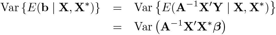
where the second equality follows from the fact that A ^{− 1} X ′ is a function of X conditional on known reliabilities and the fact that E(Y | X, X ^∗ ) = E(Y | X ^∗ ) = X ^∗β. For the second term on the right-hand side of (4),

$\begin{array}{l}\begin{array}{ll}E\{Var(b|X,X^{\ast })\}\hfill & =\hspace{0.17em}\hspace{0.17em}\hspace{0.17em}\hspace{0.17em}E\left\{\text{Var}(A^{-1}X\prime Y|X,X^{\ast })\right\}\hfill \\ \hfill & =\hspace{0.17em}\hspace{0.17em}\hspace{0.17em}E\left\{A^{-1}X\prime \text{Var}(Y|X,X^{\ast })X{A}^{-1}\right\}\hfill \\ \hfill & =\hspace{0.17em}\hspace{0.17em}\hspace{0.17em}{\sigma }^{2}E\left(A^{-1}X\prime X{A}^{-1}\right)\hfill \end{array}\\ \end{array}$

Thus, an alternate expression for Var(b) in (4) is

$\text{Var}(b) =\text{ Var}\left(A^{-1}X\prime X^{\ast }\beta \right)+{\sigma }^{2}E\left(A^{-1}X\prime X{A}^{-1}\right)$

5

The key issue is that the first term on the right-hand side of (5) is not zero in EIV regression. This deviates from OLS regression. Specifically, OLS regression corresponds to the case in which the reliabilities r_j ≡ 1 so that X ≡ X ^∗ and A ≡ X ^∗′ X ^∗ . In this case, Var(A ^{− 1} X ′ X ^∗β)= Var(β) = 0. Alternatively, when some predictors are measured with error, Var(A ^{− 1} X ′ X ^∗β) is generally positive because A ^{− 1} X ′ X ^∗ is a random matrix rather than a fixed identity matrix. ⁵ Thus, A ^{− 1} X ′ X ^∗β varies from sample to sample and contributes to variability in b rather than being identically equal to β.

The estimate $\widetilde{Var}(b)$ of Var(b) computed by eivreg ignores this term and essentially provides only an estimate of the second term on the right-hand side of (5), at least as of Stata 14.1. Specifically, $\widetilde{Var}(b)$ computed by eivreg is a plugin estimator of ${\sigma }^{2}E\left(A^{-1}X\prime X{A}^{-1}\right)$ because eivreg first computes an estimate of the residual variance σ ² of the true regression in (1) equal to

${\widehat{\sigma }}^2=\frac{Y \prime Y-b\prime Ab}{N-p}$

It then estimates Var(b) using

$\widetilde{\text{Var}}(b) ={\widehat{\sigma }}^2{A}^{-1}X\prime X{A}^{-1}$

6

The estimator ${\widehat{\sigma }}^2$ consistently estimates σ ² under standard regularity conditions because $\text{plim}\{Y\prime Y/(N-p)\}=$ $E(Y_i^2) =E(\beta \prime X_i^{\ast }{X}_i^{\ast }\prime \beta ) +E({ϵ}_i^2)$ and $\text{plim}\{b\prime Ab/(N-p)\}=E(\beta \prime X_i^{\ast }{X}_i^{\ast }\prime \beta )$ . Thus, the difference consistently estimates $E({ϵ}_i^2) ={\sigma }^2$ . The estimated variance in (6) then plugs the observed value of A ^{− 1} X ′ XA ^{− 1} in as an estimator of its expected value, so that $\widetilde{\text{Var}}(b)$ can be viewed as a plugin estimator of σ ² E(A ^{− 1} X ′ XA ^{− 1}). This is the second term on the right-hand side of (5), while the first term is implicitly ignored.

The fact that σ ² E(A ^{− 1} X ′ XA ^{− 1})equals E{Var(b | X, X ^∗ )} means that $\widetilde{\text{Var}}(b)$ reported by eivreg is appropriate only under the assumption that all covariates and their corresponding measurement errors are fixed. This assumption generally would be inconsistent with random sampling of units from a population and is particularly restrictive in applications with measurement error because it also conditions on fixed values of unobserved measurement errors. Moreover, even in applications where these assumptions would be warranted, the variance estimator used by eivreg would be appropriate for characterizing the sampling variability of the estimated regression coefficients but would not be appropriate for characterizing the mean squared error of these estimators because E(b | X, X ^∗ ) generally does not equal β. Alternatively, $\widehat{\text{Var}}(b)$ as reported by sem yields standard-error estimators that are consistent with random sampling of the covariates, measurement errors, and outcomes from a population distribution, implicitly accounting for both terms in (5).

2.4 Magnitude of bias for eivreg standard errors

It is difficult to evaluate the relative magnitude of the two terms in (5) in general, but some basic results are evident. For fixed N and fixed σ ², as r_j → 1 for j = 1,…, p, Var(A ^{− 1} X ′ X ^∗β) converges to zero and σ ² E(A ^{− 1} X ′ XA ^{− 1})converges to σ ² E (X ^∗′ X ^∗ )−1, the variance of the OLS estimator of β under random sampling of all variables.

Note also that Var(A ^{− 1} X ′ X ^∗β) does not depend on σ ². Thus, for fixed N and fixed reliabilities that are less than 1, as σ ² → 0, this term dominates the variance. Because eivreg ignores this term, the standard errors reported by eivreg will tend to be more negatively biased when σ ² is small, or alternatively, when the R ² of the true regression is large. For fixed N and fixed σ ², it is difficult to discern the relative magnitude of the two terms as the reliabilities change because both terms are affected by the reliabilities.

A key consideration is the relative magnitude of the terms as N changes, for fixed σ ² and fixed reliabilities. The general results from estimating equation theory indicate that, under sufficient regularity conditions, b is consistent and asymptotically normal with variance that is O(1/N). Thus, both terms in (5) must converge to zero as N goes to infinity. However, it is unclear from the expressions under what conditions the two terms will decrease at the same rate as a function of N. It can be shown that both terms are O(1/N) in a simple case with a scalar, normally distributed latent predictor $X_i^{\ast }$ with known mean zero and normally distributed measurement errors U_i . In this case, $\widetilde{\text{Var}}(b)/Var(b)$ will generally remain less than 1 as N increases, where b is the estimated coefficient on $X_i^{\ast }$ . This would mean that eivreg standard errors will underestimate the true standard errors in expectation, and the coverage rate of the associated confidence intervals will be less than the nominal level, regardless of the sample size.

3 Simulation study

We conducted a simple simulation study to demonstrate the practical differences between the standard errors reported by eivreg and those reported by sem. We consider the case where p = 2 (that is, an intercept and a scalar predictor) and focus only on the estimated coefficient for the predictor. Our simulation varied three factors: the sample size N, the R ² of the true regression, and the reliability r. Specifically, we considered four sample sizes N of 100, 500, 1,000, and 5,000; five values of R ² for the true regression of 0.10, 0.30, 0.50, 0.70, and 0.90; and five reliabilities r of 0.50, 0.60, 0.70, 0.80, and 0.90, for a total of 100 simulation conditions. For each of the 100 simulation conditions, we used 1,800 independent Monte Carlo replications. ⁶ For each replication, the observed predictor X_i for i = 1,…, N was generated as $X_i=X_i^{\ast } +\hspace{0.17em}{U}_i$ , where the latent predictor $X_i^{\ast }$ was normally distributed with mean zero and variance one, and the measurement error U_i was normally distributed with mean zero and variance (1 − r)/r. Then, Y_i was set equal to 0.0+1.0 $X_i^{\ast } +\hspace{0.17em}{ϵ}_i$ , where ϵ_i was normally distributed with mean zero and variance (1 − R ²)/R ². Thus, the coefficient β on $X_i^{\ast }$ in the true regression was equal to 1.0.

For each simulation condition and Monte Carlo replication, we used the simulated data to compute the EIV regression estimate b of β and its associated standard-error estimate, using both eivreg and sem. ⁷ For eivreg, we tracked both the reported standard error for b and the standard error estimated using bootstrapping with 250 independent bootstrap replications. We used 250 bootstrap samples because that amount should be more than sufficient in most cases per Efron and Tibshirani (1993, 52), but the computational time was not prohibitive.

For each of the three standard-error estimation methods (sem-reported standard errors, eivreg-reported standard errors, bootstrapped standard errors), we then computed the 95% confidence interval for β and tracked whether the confidence interval contained the true value of β = 1. For each of the 100 simulation conditions, we estimated the coverage probability of the 95% confidence intervals by averaging over the 1,800 Monte Carlo replications. For each of the 100 simulation conditions, we also computed the ratio of the mean standard error reported by eivreg across the 1,800 replications to the sample standard deviation of b across the replications. When this ratio is less than 1, it indicates that the reported standard errors tend to be smaller than the actual standard deviation of the sampling distribution of b. We computed the analogous ratio using the bootstrapped standard errors and the standard errors reported by sem. The simulation was run in Stata 14.1 for Linux, and the code is provided in the appendix.

In initial explorations of the simulation study, we found simulated datasets for which the EIV regression estimator exists and was successfully computed by eivreg but for which sem did not converge to this solution from its default starting values. Thus, as demonstrated in the code in the appendix, we modified the call to sem to use the MLEs of the model parameters as starting values. The MLE of the regression coefficient for $X_i^{\ast }$ was computed by eivreg, and MLEs of the required variance components were computed using this regression coefficient, the reliability, and sample variances of Y_i and X_i for i = 1,…, N. As expected, initializing the parameters in this way led to rapid convergence of sem and estimated regression coefficients across sem and eivreg that demonstrated only negligible numerical differences for all simulated datasets.

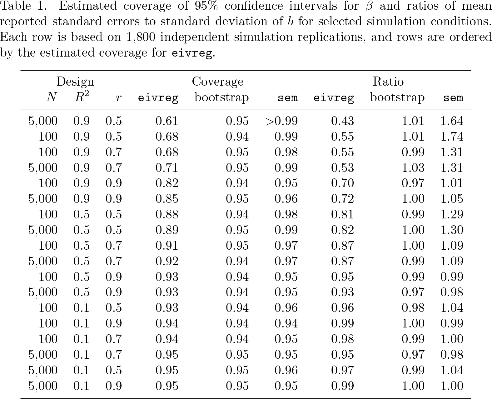
The simulation results were consistent with the analytical results regarding the negative bias in the standard-error estimators reported by eivreg. The 95% confidence intervals for β using the standard errors reported by eivreg had less than 95% coverage. Across the 100 simulation conditions, the coverage probabilities using the standard errors reported by eivreg ranged from 0.58 to 0.95 with mean 0.87. Coverage was worse when R ² was large and r was small, regardless of sample size N. The coverage approached the nominal levels when R ² was small and r was large, again regardless of N. The ratio of the mean standard errors reported by eivreg to the estimated sampling standard deviation of b ranged from 0.42 to 1.02 with mean 0.82, consistent with the undercoverage of the confidence intervals.

Alternatively, confidence intervals computed using either the standard errors reported by sem or the bootstrapped standard errors had closer to nominal coverage. For sem, coverage ranged from 0.94 to greater than 0.99, with mean 0.97. The ratio of the mean standard errors reported by sem to the estimated sampling standard deviation of b ranged from 0.95 to 1.74, with mean 1.14, consistent with the confidence interval coverage that somewhat exceeds the nominal level. For the bootstrapped standard errors, coverage ranged from 0.92 to 0.96, with mean 0.95, and the ratios of mean standard errors to estimated sampling standard deviation of b ranged from 0.95 to 1.05, with mean 0.99. Table 1 provides results from the three standard-error estimation methods for a representative subset of the 100 simulation conditions, with rows ordered according to the coverage for eivreg.

Table 1.

Estimated coverage of 95% confidence intervals for β and ratios of mean reported standard errors to standard deviation of b for selected simulation conditions. Each row is based on 1,800 independent simulation replications, and rows are ordered by the estimated coverage for eivreg.

Design				Coverage			Ratio
N	R 2	r	eivreg	bootstrap	sem	eivreg	bootstrap	sem
5,000	0.9	0.5	0.61	0.95	>0.99	0.43	1.01	1.64
100	0.9	0.5	0.68	0.94	0.99	0.55	1.01	1.74
100	0.9	0.7	0.68	0.95	0.98	0.55	0.99	1.31
5,000	0.9	0.7	0.71	0.95	0.99	0.53	1.03	1.31
100	0.9	0.9	0.82	0.94	0.95	0.70	0.97	1.01
5,000	0.9	0.9	0.85	0.95	0.96	0.72	1.00	1.05
100	0.5	0.5	0.88	0.94	0.98	0.81	0.99	1.29
5,000	0.5	0.5	0.89	0.95	0.99	0.82	1.00	1.30
100	0.5	0.7	0.91	0.95	0.97	0.87	1.00	1.09
5,000	0.5	0.7	0.92	0.94	0.97	0.87	0.99	1.09
100	0.5	0.9	0.93	0.94	0.95	0.95	0.99	0.99
5,000	0.5	0.9	0.93	0.94	0.95	0.93	0.97	0.98
100	0.1	0.5	0.93	0.94	0.96	0.96	0.98	1.04
100	0.1	0.9	0.94	0.94	0.94	0.99	1.00	0.99
100	0.1	0.7	0.94	0.94	0.95	0.98	0.99	1.00
5,000	0.1	0.7	0.95	0.95	0.95	0.95	0.97	0.98
5,000	0.1	0.5	0.95	0.95	0.96	0.97	0.99	1.04
5,000	0.1	0.9	0.95	0.95	0.95	0.99	1.00	1.00

4 Conclusion

The findings of this article indicate that Stata provides at least two alternatives to using eivreg with its reported standard errors that are likely to be preferable in most applications with error-prone covariates: eivreg with bootstrapped standard errors and sem. We discuss each alternative in turn.

Regarding bootstrapping, because the method-of-moments estimator implemented by eivreg is fast and relatively robust, combining eivreg with bootstrapping may be attractive in some applications. Although our simulation studies considered only a simple case, it seems reasonable to expect that bootstrapping would perform well even in more complicated settings (for example, multiple error-prone and error-free covariates). As such, Stata could consider adding a vce(bootstrap) option to eivreg in future releases to encourage eivreg users to consider this option in their applications.

Regarding the use of sem for EIV regression, this option is attractive not only because sem provides standard errors consistent with random sampling of all relevant quantities, but also because it is more flexible than eivreg. For example, sem can handle missing data when they are missing at random (whereas eivreg drops cases with incomplete data); it provides several methods for standard-error estimation in more complicated settings such as heteroskedasticity and clustering of residual errors (whereas eivreg provides no such options); and it can accommodate nondiagonal variance–covariance matrices for the measurement errors (whereas eivreg requires uncorrelated measurement errors). The main disadvantages of sem relative to eivreg are that it is slower and does not always converge from its default starting values even for datasets in which the EIV estimator exists. The latter problem could be addressed by using eivreg to generate starting values for sem to achieve convergence in difficult cases.

An additional limitation of sem is worth noting. When reliabilities are treated as known, sem uses those reliabilities to compute estimates of the measurement error variances and then treats those estimated measurement error variances as known when computing $\widehat{\text{Var}}(b)$ . Thus, there is a mismatch between what is actually fixed (the reliabilities) and what is treated as fixed (the measurement error variances) in the calculation of $\widehat{\text{Var}}(b)$ . This could explain why the reported standard errors from sem summarized in table 1 were too large for some simulation conditions. We conducted an auxiliary simulation study that supported this conjecture. Specifically, we ran a version of the simulation study in which sem was invoked using a known measurement error variance rather than a known reliability. That is, for a simulation condition with reliability r, our modified simulation study applied sem by specifying the measurement error variance as known and equal to (1 − r)/r, rather than by specifying the reliability as known and equal to r. Across simulation conditions, the coverage of the 95% confidence intervals averaged 0.95, and the ratio of the mean standard errors reported by sem to the estimated sampling standard deviation of b averaged 1.00. These results suggest that the overcoverage for sem demonstrated in table 1 will not occur in cases where sem is applied with known measurement error variances rather than known reliabilities. The code for this simulation study is available from the authors by request. The results also suggest that it may be valuable to modify the sem standard-error calculations when reliabilities rather than measurement error variances are specified by the user. One approach to such modification is to include the estimation of the measurement error variances from the marginal variances of the observed predictors and the assumed reliabilities as additional equations in the system of estimating equations determining the MLE and to use standard results from M estimation (for example, Stefanski and Boos [2002]) to estimate the standard errors.

These considerations also suggest a possible advantage of bootstrapped standard errors when the reliabilities are treated as known because the bootstrap distribution of b is based on holding the reliabilities constant. Thus, the sampling distribution of b is approximated under conditions that are consistent with what the analyst is treating as known. The results of table 1 appear to provide an example of this possible advantage of bootstrapping because it does not appear to be susceptible to overcoverage.

Finally, our simulation study considered only the simplest possible case of EIV regression with a single error-prone covariate, no other covariates, and a joint Gaussian distribution for all quantities of interest. Given the theoretical considerations, we expect that the deficiencies of the standard errors estimated by eivreg will carry over to more general cases, but further study of these deficiencies and the performance of both sem and bootstrapping would be warranted.

References

1.
BollenK. A.1989. Structural Equations with Latent Variables. New York: Wiley.
CarrollR. J.RuppertD.StefanskiL. A.CrainiceanuC. M.2006. Measurement Error in Nonlinear Models: A Modern Perspective. 2nd ed. Boca Raton, FL: Chapman & Hall/CRC.
4.
CulpepperS. A.AguinisH.2011. Using analysis of covariance (ANCOVA) with fallible covariates. Psychological Methods16: 166–178. https://doi.org/10.1037/a0023355.
5.
EfronB.TibshiraniR. J.1993. An Introduction to the Bootstrap. New York: Chapman & Hall/CRC.
6.
FullerW. A.1987. Measurement Error Models. New York: Wiley.
7.
FullerW. A.HidiroglouM. A.1978. Regression estimation after correcting for attenuation. Journal of the American Statistical Association73: 99–104. https://doi.org/10.2307/2286529.
8.
LockwoodJ. R.McCaffreyD. F.2014. Correcting for test score measurement error in ANCOVA models for estimating treatment effects. Journal of Educational and Behavioral Statistics39: 22–52. https://doi.org/10.3102/1076998613509405.
9.
LordF. M.1980. Applications of Item Response Theory to Practical Testing Problems. Hillsdale, NJ: Lawrence Erlbaum.
ToddP. E.WolpinK. I.2003. On the specification and estimation of the production function for cognitive achievement. Economic Journal113: F3–F33. https://doi.org/10.1111/1468-0297.00097.