Sage Journals: Discover world-class research

Abstract

The wild bootstrap was originally developed for regression models with heteroskedasticity of unknown form. Over the past 30 years, it has been extended to models estimated by instrumental variables and maximum likelihood and to ones where the error terms are (perhaps multiway) clustered. Like bootstrap methods in general, the wild bootstrap is especially useful when conventional inference methods are unreliable because large-sample assumptions do not hold. For example, there may be few clusters, few treated clusters, or weak instruments. The package boottest can perform a wide variety of wild bootstrap tests, often at remarkable speed. It can also invert these tests to construct confidence sets. As a postestimation command, boottest works after linear estimation commands, including regress, cnsreg, ivregress, ivreg2, areg, and reghdfe, as well as many estimation commands based on maximum likelihood. Although it is designed to perform the wild cluster bootstrap, boottest can also perform the ordinary (nonclustered) version. Wrappers offer classical Wald, score/Lagrange multiplier, and Anderson–Rubin tests, optionally with (multiway) clustering. We review the main ideas of the wild cluster bootstrap, offer tips for use, explain why it is particularly amenable to computational optimization, state the syntax of boottest, artest, scoretest, and waldtest, and present several empirical examples.

Keywords

st0549 boottest artest waldtest scoretest Anderson–Rubin test Wald test wild bootstrap wild cluster bootstrap score bootstrap multiway clustering few treated clusters

1 Introduction

It is common in social science research to assume that the error terms in regression models are correlated within clusters. These clusters might be, for example, jurisdictions, villages, firm types, classrooms, schools, or time periods. This is why many Stata estimation commands offer a cluster option to implement a cluster–robust variance matrix estimator (CRVE) that is robust to both intracluster correlation and heteroskedasticity of unknown form. Inference based on the standard errors produced by this option can work well when large-sample theory provides a good guide to the finite-sample properties of the CRVE. This will typically be the case if the number of clusters is large, if the clusters are reasonably homogeneous in size and covariance structure, and—for regressions estimating treatment effects—if the number of treated clusters is not too small. But inference can sometimes be misleading when these conditions do not hold.

One way to improve inference when large-sample theory provides a poor guide is to use the bootstrap. The idea is to generate many bootstrap samples that mimic the distribution from which the actual sample was obtained. Each of them is then used to compute a bootstrap test statistic, using the same test procedure as for the original sample. The bootstrap p-value is then calculated as the proportion of the bootstrap statistics that are more extreme than the actual one from the original sample. See, among many others, Davison and Hinkley (1997) and MacKinnon (2009) for a general introduction.

In general, bootstrap inference will be more reliable the more closely the bootstrap data-generating process (DGP) matches the (unknown) true DGP; see Davidson and MacKinnon (1999). For many regression models, the wild bootstrap (Wu 1986; Liu 1988) frequently does a good job of matching the true DGP. It is implemented by multiplying the residuals from the original linear model by certain random weights to construct bootstrap samples with dependent variables that are related to the independent variables by the same linear model. Cameron, Gelbach, and Miller (2008), hereafter CGM (2008), adapted this approach to models with clustered errors, holding the random weights fixed within each cluster in each bootstrap replication. Simulation evidence suggests that bootstrap tests based on the wild and wild cluster bootstraps often perform well; see, among others, Davidson and MacKinnon (2010), MacKinnon (2013), and MacKinnon and Webb (2017a).

A less well-known strength of the wild bootstrap is that, in many important cases, its simple and linear mathematical form lends itself to extremely fast implementation. As we will explain in section 5, the combined algorithm for generating many bootstrap replications and computing a test statistic for each of them can often be condensed into a few matrix formulas. For the linear regression model with clustered errors, viewing the process in this way opens the door to fast implementation of the wild cluster bootstrap.

The postestimation command boottest, written and maintained by one of us (Roodman), implements several versions of the wild cluster bootstrap. These include the ordinary (nonclustered) wild bootstrap as a special case. boottest supports

inference after ordinary least-squares (OLS) estimation with regress;

inference after restricted OLS estimation with cnsreg;

inference using the wild restricted efficient (WRE) bootstrap of Davidson and MacKinnon (2010) for two-stage least-squares (2SLS), limited-information maximum likelihood (LIML), and other instrumental variable (IV) methods, as with ivregress and ivreg2 (Baum, Schaffer, and Stillman 2007);

inference after maximum likelihood (ML) estimation via the “score bootstrap” (Kline and Santos 2012) with such ML-based commands as probit, logit, glm, sem, gsem, and the community-contributed command cmp (Roodman 2011);

multiway clustering, even after estimation commands that do not support it;

models with one-way fixed effects (FEs), estimated with areg, reghdfe (Correia 2014), xtreg, xtivreg, or xtivreg2 with the fe option;

inversion of tests of one-dimensional hypotheses to derive confidence sets; and

plotting of the corresponding confidence functions.

Section 2 of this article describes the linear regression model with one-way clustering and explains how to compute cluster–robust variance matrices. Section 3 describes the key ideas of the wild cluster bootstrap and then introduces several variations and extensions. Section 4 discusses multiway clustering and associated bootstrap methods. Section 5 explains the techniques implemented in boottest to speed up execution of the wild cluster bootstrap, especially when the number of clusters is small relative to the number of observations. Section 6 discusses extensions to IV estimation and to ML estimation. Section 7 describes the syntax of the boottest package. Finally, section 8 illustrates how to use the program in the context of some empirical examples.

2 Regression models with one-way clustering

Consider the linear regression model

y = X β + u

where y and u are N × 1 vectors of observations and error terms, respectively, X is an N × k matrix of covariates, and β is a k × 1 parameter vector. The observations are grouped into G clusters, within each of which the error terms may be correlated. Model (1) can be rewritten as

y_{g} = X_{g} β + u_{g}, g = 1, . . ., G

where the vectors y _g and u _g and the matrix X _g contain the rows of y, u, and X that correspond to the gth cluster. Each of these objects has N_g rows, where N_g is the number of observations in cluster g.

Conditional on X, the vector of error terms u has mean zero and variance matrix Ω = E(uu′ | X), which is subject to the key assumption of no cross-cluster correlation:

E (u_{g} {u^{'}}_{h} | X) = 0 if g \neq h

Thus, Ω is block-diagonal with blocks Ω _g = E(u _g u _g ′ | X). We make no assumptions about the entries in these blocks, except that each of the Ω _g is a valid variance matrix (positive definite and finite).

The OLS estimator of β is

\hat{β} = {(X^{'} X)}^{- 1} X^{'} y

and the vector of estimation residuals is

\hat{u} = y - X \hat{β}

The conditional variance matrix of the estimator $\hat{β}$ is

var (\hat{β} | X) = {(X^{'} X)}^{- 1} X^{'} Ω X {(X^{'} X)}^{- 1}

This expression cannot be computed, because it depends on Ω, which by assumption is not known. The feasible analog of (5) is the CRVE of Liang and Zeger (1986). It replaces Ω by the estimator $\hat{Ω}$ , which has the same block-diagonal form as Ω, but with ${\hat{Ω}}_{g} = {\hat{u}}_{g} {\hat{u}}^{'}_{g}$ for g = 1,…, G. This leads to the CRVE

\hat{V} = m {(X^{'} X)}^{- 1} X^{'} Ω X {(X^{'} X)}^{- 1}, \hat{Ω} = blockdiag ({\hat{Ω}}_{1}, . . ., {\hat{Ω}}_{G})

where the scalar finite-sample adjustment factor, m, will be defined below. The center factor in (6) is often more conveniently computed as

X^{'} \hat{Ω} X = \sum_{g = 1}^{G} {X^{'}}_{g} {\hat{u}}_{g} {\hat{u}}^{'}_{g} X_{g}

It should be clear that $\hat{Ω}$ is in no sense a consistent estimator of Ω, because both are N × N matrices. However, the “sandwich” estimator $\hat{V}$ defined in (6) is consistent, in the sense that the inverse of the true variance matrix defined in (5) times $\hat{V}$ converges to an identity matrix as G → ∞. A proof of the consistency of the CRVE for general one-way clustering under weak distributional assumptions that allow both G and the N_g to increase with N is provided in Djogbenou, MacKinnon, and Nielsen (2018).¹

When the error terms in the regression model (1) are potentially heteroskedastic, but uncorrelated, we have the “robust” case in informal Stata parlance. This is a special case of the clustered model (2) in which each cluster contains just one observation. For this model, the CRVE is simply the heteroskedasticity-robust variance estimator of Eicker (1963) and White (1980).

We now write $\hat{Ω}$ in a way that will facilitate our discussion of fast computation in section 5. We define S as the G × N matrix that by left-multiplication sums the columns of a data matrix clusterwise. For example, SX is the G × k matrix of clusterwise sums of the columns of X. Note that S′S is the N × N indicator matrix whose (i, j)th entry is 1 or 0 according to whether observations i and j are in the same cluster. Leftmultiplying by S′ expands a matrix with one row per cluster to a matrix with one row per observation by duplicating entries within each cluster.

We also adopt notation used for the family of colon-prefixed “broadcasting” operators in Stata’s matrix programming language, Mata. For example, if A and B have the same dimensions, then A :* B is the Hadamard (elementwise) product. But if v is a column vector while B is a matrix, and if the two have the same number of rows, then v :* B is the columnwise Hadamard product of v with the columns of B. As in Mata, we give :* lower precedence than ordinary matrix multiplication. For later use, we note that, if v is a column vector, then the :* operator obeys the identities

(v : * A)' = A' : * v' = v' : * A'

v : * A B = (v : * A) B

A B : * v' = A (B : * v')

A (v : * B) = (A : * v') B

In terms of these constructs, the CRVE in (6) is

\hat{V} = m {(X^{'} X)}^{- 1} X^{'} Ω X {(X^{'} X)}^{- 1}, \hat{Ω} = \hat{u} : * S^{'} S : * {\hat{u}}^{'}

By Stata convention, the small-sample correction m in (6) and (12) is

m = \frac{G}{G - 1} \times \frac{N - 1}{N - k}

This choice has the intuitive property that, in the limiting case of G = N, that is, the “robust” case, the expression reduces to the classical N/(N − k) correction factor.

The CRVE in (12) allows for the possibility that individual observations within each cluster are not independent of each other. In other words, for purposes of estimation, the effective sample size may be less than the formal sample size N. In the extreme case of complete within-group dependence, the cluster becomes the effective unit of observation, and the effective sample size becomes G.

The large-sample theory of the CRVE (Carter, Schnepel, and Steigerwald 2017; Djogbenou, MacKinnon, and Nielsen 2018) is based on the assumption that G → ∞ rather than N → ∞.² This appears to be why Stata has long used the t(G − 1) distribution to obtain p-values for cluster–robust t statistics, a practice supported by the theory in Bester, Conley, and Hansen (2011). However, this theory can be misleading when G is small or when the clusters differ greatly in size or in the structure of their variance matrices or (in the treatment case) when there are few treated clusters. In some cases, it can result in severe overrejection. Simulation results that show the severity of this overrejection may be found in MacKinnon and Webb (2017b, 2018) and Djogbenou, MacKinnon, and Nielsen (2018), among others. In extreme cases, tests at the 0.05 level can reject well over 60% of the time.

The “effective number of clusters” developed in Carter, Schnepel, and Steigerwald (2017) often provides a useful diagnostic, which can be computed using the package clusteff; see Lee and Steigerwald (2018). Inference based on the t(G−1) distribution is likely to be unreliable when G ^∗, the effective number of clusters, is much smaller than G, especially when G ^∗ is less than about 20. In such cases, the wild cluster bootstrap and the t(G − 1) distribution may yield inferences that differ sharply. However, there is no reason to restrict the use of the wild cluster bootstrap to such cases. Because boottest is so fast, we recommend using it all the time, at least for final results.

3 The wild cluster bootstrap

Bootstrap methods for hypothesis testing involve generating many bootstrap samples that resemble the actual one, computing the test statistic for each of them, and then deciding how extreme the original test statistic is by comparing it with the distribution of the bootstrap test statistics. This sort of bootstrapping often works well. In some cases, it provides an asymptotic refinement, which means that, as the sample size increases, the bootstrap distribution approaches the actual distribution faster than does the asymptotic distribution that is normally relied upon (such as the t or chi-squared). This type of theoretical result holds for test statistics that are asymptotically pivotal, such as most t statistics.

In this section, we discuss the wild cluster bootstrap, which was proposed in CGM (2008) and the validity of which was proved in Djogbenou, MacKinnon, and Nielsen (2018). It is a generalization of the ordinary wild bootstrap, which was developed in Liu (1988) for the nonclustered, heteroskedastic case, following a suggestion in Wu (1986) and commentary thereon by Beran (1986). H¨ ardle and Mammen (1993) appear to have been the first to call the method “wild”, observing that it “…can be thought of as attempting to reconstruct the distribution of each residual through the use of one single observation.”

3.1 The algorithm

The bootstrap method most deeply embedded in Stata—via the bootstrap prefix command—is a nonparametric bootstrap that, when applied to regression models, is often called the “pairs bootstrap”. In the estimation context set out in the previous section, this bootstrap would typically operate by resampling (y _g, X _g ) pairs at the cluster level (Field and Welsh 2007). This is asymptotically valid, but some of the bootstrap samples may not resemble the actual sample, especially if the cluster sizes vary a lot. In a difference-in-differences context with few treated clusters, the treatment dummy could even equal zero for all observations in some bootstrap samples. For these reasons, the pairs cluster bootstrap can work poorly in some cases; see Bertrand, Duflo, and Mullainathan (2004) and MacKinnon and Webb (2017a).

In the wild cluster bootstrap, all the bootstrap samples have the same covariates X. If the bootstrap samples are denoted by an asterisk and indexed by b, only the bootstrap error vector u ^∗ ^b , and hence also the bootstrap dependent variable y ^∗ ^b , differs across them. In particular, the vectors y ^∗ ^b are generated, cluster by cluster, as

y_{g}^{* b} = X_{g} \ddot{β} + u_{g}^{* b}, u_{g}^{* b} = v_{g}^{* b} ü_{g}

where $\ddot{β}$ is an estimate of β and ü _g is the vector of residuals for cluster g computed using $\ddot{β}$ . The scalar $v_{g}^{* b}$ is an auxiliary random variable with mean 0 and variance 1, sometimes referred to as a “wild weight”. It is often drawn from the Rademacher distribution, meaning that it takes the values −1 and +1 with equal probability. The choice of $\ddot{β}$ , and hence also ü _g , will be discussed just below. Using the matrix S defined above, we can rewrite the wild bootstrap DGP as

y^{* b} = X \ddot{β} + u^{* b}, u^{* b} = ü : * S' v^{* b}

where v ^∗ ^b is a G × 1 vector with gth element $v_{g}^{* b}$ .

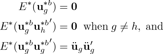
Because the $v_{g}^{* b}$ are independent of X and the ü _g and have mean 0 and variance 1, multiplying the ü _g by $v_{g}^{* b}$ as in (14) preserves the first and second moments of the ü _g . Specifically, let E ^∗ denote expectation conditional on the data, y and X, so that only the $v_{g}^{* b}$ are treated as random. Then it is not difficult to see that

\begin{array}{l} E^{*} (u_{g}^{* b}) = 0 \\ E^{*} (u_{g}^{* b} u_{h}^{* b^{'}}) = 0 w h e n g \neq h, a n d \\ E^{*} (u_{g}^{* b} u_{h}^{* b^{'}}) = {\ddot{u}}_{g} {\ddot{u}}_{g}^{'} \end{array}

Up to this point, we have used $\ddot{β}$ and ü to denote vectors of parameter estimates and residuals, without specifying precisely how they are computed. One possibility is that $\ddot{β} = \hat{β}$ and $\ddot{u} = \hat{u}$ , where $\hat{β}$ is the vector of OLS estimates for the model (1) and $\hat{u}$ is the associated vector of residuals. Another possibility is that $\ddot{β} = \tilde{β}$ and $\ddot{u} = \hat{u}$ , where $\hat{β}$ denotes least-squares estimates of (1) subject to whatever restriction or restrictions are to be tested and $\tilde{u}$ denotes the associated vector of residuals. For example, if we wish to test whether β_j = 0, where β_j is the jth element of β, we would set ${\tilde{β}}_{j} = 0$ and obtain the remaining elements of $\tilde{β}$ by regressing y on every column of X except the jth.

These two choices lead to two variants of the wild cluster bootstrap, which we call wild cluster unrestricted (WCU) and wild cluster restricted (WCR). CGM (2008) referred to WCR as the wild cluster bootstrap with the null imposed. Section 3.2 discusses why it is generally better to use the WCR variant. To explain how both work, we continue to use the generic notation $\ddot{β}$ and ü.

For concreteness, we suppose that our objective is to test the hypothesis that β_j = 0. Then the WCU and WCR algorithms are as follows:

1. Regress y on X to obtain $\hat{β}, \hat{u}, a n d \hat{V}$ , as given in (3), (4), and (12).

2. Calculate the usual cluster–robust t statistic for the hypothesis that β_j = 0,

t_{j} = \frac{\hat{β}}{\sqrt{{\hat{V}}_{j j}}}

where ${\hat{V}}_{j j}$ is the jth diagonal element of $\hat{V}$ .

3. For the WCU bootstrap, set $\ddot{β} = \hat{β} and \ddot{u} = \hat{u}$ . For the WCR bootstrap, regress y on X subject to the restriction that β_j = 0 to obtain $\tilde{β} and \tilde{u} and set \ddot{β} = \tilde{β} and \ddot{u} = \tilde{u}$ .

4. For each of B bootstrap replications:

Using (15), generate a new set of bootstrap error terms u ^∗ ^b and dependent variables y ^∗ ^b .

By analogy with step 1, regress y ^∗ ^b on X to obtain ${\hat{β}}^{* b} and {\hat{u}}^{* b}$ , and use the latter in (12) to compute the bootstrap CRVE ${\hat{V}}^{* b}$ .

Calculate the bootstrap t statistic for the null hypothesis that $β_{j}^{* b} = {\ddot{β}}_{j}$ as

t_{j}^{* b} = \frac{{\hat{β}}_{j}^{* b} - {\ddot{β}}_{j}}{\sqrt{{\hat{V}}_{j j}^{* b}}}

where ${\hat{V}}_{j j}^{* b}$ is the jth diagonal element of ${\hat{V}}^{* b}$ . For the WCR bootstrap, the numerator of (17) can also be written as ${\hat{β}}_{j}^{* b} because {\ddot{β}}_{j} = 0$ .

5. For a one-tailed test, use the distribution of all the $t_{j}^{* b}$ to compute the lower-tail or upper-tail p-value,

{\hat{P}}_{L}^{*} = \frac{1}{B} \sum_{b=1}^{B} I (t_{j}^{* b} < t_{j}) or {\hat{P}}_{U}^{*} = \frac{1}{B} \sum_{b=1}^{B} I (t_{j}^{* b} > t_{j})

where $I$ (·) is the indicator function. For a two-tailed test, compute either the symmetric or the equal-tail p-value,

{\hat{P}}_{S}^{*} = \frac{1}{B} \sum_{b=1}^{B} I ({|t}_{j}^{* b} | > | t_{j} |) or {\hat{P}}_{ET}^{*} = 2 \min ({\hat{P}}_{L}^{*}, {\hat{P}}_{U}^{*})

The former is appropriate if the distribution of t_j is symmetric around a mean of zero. In that case, if B is not very small, ${\hat{P}}_{S}^{*} and {\hat{P}}_{ET}^{*}$ will be similar. If the symmetry assumption is violated, which it will be when ${\hat{β}}_{j}$ is biased, it is better to use ${\hat{P}}_{ET}^{*}$ . Asymmetry becomes a greater concern when we extend the wild cluster bootstrap to IV estimation in section 6.1 because IV estimators are biased toward the corresponding OLS estimators.

We make a few observations on this algorithm. First, whether the WCR or WCU bootstrap is used in step 3, the t statistic calculated in step 4c tests a hypothesis, $β_{j} = {\ddot{β}}_{j}$ , that is true by construction in the bootstrap samples because $\ddot{β}$ is used to construct the samples in step 4a. Because the bootstrap distribution is generated by testing a null hypothesis on samples from a DGP for which the null is correct, the resulting bootstrap distribution should mimic the distribution of the sample test statistic, t_j , when the null hypothesis of interest, β_j = 0, is also correct.

Second, because the small-sample correction factor m defined in (13) and used in the CRVE (12) affects both t_j and the $t_{j}^{* b}$ proportionally, the choice of m does not affect any of the bootstrap p-values.

Third, the algorithm does not produce standard errors (which is why boottest does not attempt to compute them). Instead, inference is based on p-values and confidence sets; the latter are discussed below in section 3.5. One could compute the standard deviation of the bootstrap distribution of ${\hat{β}}^{* b}$ and then use it for inference in several ways. However, this approach relies heavily on the asymptotic normality of $\hat{β}$ in a case where large-sample theory may not apply. Higher-order asymptotic theory for the bootstrap (Davison and Hinkley 1997, chap. 5) predicts that this approach should not perform as well as the algorithm discussed above, and Monte Carlo simulations in CGM (2008) confirm this prediction.

The last observation relates to the number of bootstrap samples, B. Given a significance level α, it is usually desirable to choose B such that α(B + 1) is an integer (Davidson and MacKinnon 2004, 163–164). To see why, suppose that we violate this condition by setting B = 20 and α = 0.05 when we are performing a one-sided test using ${\hat{P}}_{U}^{*}$ in (18). We could form a sorted list containing the actual test statistic t_j and the bootstrap statistics $t_{j}^{* b}$ ; this list would have 21 members. If t_j and the $t_{j}^{* b}$ obey the same distribution (which is true asymptotically under the null, and we assume is approximately true in finite samples), then t_j is equally likely to take any rank in the sorted list. As a result, ${\hat{P}}_{U}^{*}$ can take on just 21 possible values, with equal probability: 0.0, 0.05, 0.10,…, 1.0. Only the first of these would result in ${\hat{P}}_{U}^{*} < 0.0 5$ . Thus, the probability of rejecting the null would be 1/21, and not the desired 1/20. But if instead we set B = 19, ${\hat{P}}_{U}^{*}$ could take on 20 values, and the probability of rejecting the null would be exactly 1/20. For nearly the same reason, if we are using the equal-tail p-value defined in (19), we should choose α(B + 1)/2 to be an integer.

The argument in the previous paragraph hides one complication: it implicitly assumes that t_j equals any of the $t_{j}^{* b}$ with probability zero. However, there are only 2 ^G unique sets of draws for the Rademacher distribution. One of these has $v_{g}^{* b} = 1$ for all g, so that the corresponding bootstrap sample is the same as the actual sample. Therefore, each of the $t_{j}^{* b}$ equals t_j with probability 2⁻ ^G .³ When this happens, it is not entirely clear how to compute a bootstrap p-value; see Davison and Hinkley (1997, chap. 4) for a discussion of this issue. The most conservative approach is to change the strict inequalities in (18) and (19) into nonstrict ones, which would cause the p-value to be larger whenever t_j equaled any of the $t_{j}^{* b}$ . boottest does not currently do so. To avoid the problem of having t_j equal any of the $t_{j}^{* b}$ with nontrivial probability, one should use another auxiliary distribution instead of the Rademacher when G is small; see section 3.4.

3.2 Imposing the null on the bootstrap DGP

The bootstrap algorithm defined above lets the wild bootstrap DGP (15) either impose the restriction being tested (WCR) or not (WCU). Usually, it is better to impose the restriction. For any bootstrap DGP like (15) that depends on estimated parameters, those parameters are estimated more efficiently when restricted estimates are used (Davidson and MacKinnon 1999). Intuitively, because inference involves estimating the probabilities of obtaining certain results under the assumption that the null is true, inference is improved by using bootstrap datasets in which the null in fact holds. Simulation evidence on this issue is presented in, among many others, Davidson and MacKinnon (1999) and Djogbenou, MacKinnon, and Nielsen (2018).

For this reason, boottest uses the restricted estimates $\tilde{β}$ and restricted residuals $\tilde{u}$ by default.⁴ Nevertheless, boottest does allow the use of unrestricted estimates. This can be useful because WCU makes it possible to invert a hypothesis test to calculate confidence intervals for all parameters using just one set of bootstrap samples, whereas WCR requires constructing many sets of bootstrap samples to do so; see Davidson and MacKinnon (2004, sec. 5.3) and section 3.5. Thus, if the computational cost of WCR is prohibitive (although it rarely is with boottest), WCU is a practical alternative.

3.3 General and multiple linear restrictions

The algorithm given above for wild cluster bootstrap inference is readily generalized to hypotheses involving any number of linear restrictions on β. We can express a set of q such restrictions as

H_{0} : R β = r

where R and r are fixed matrices of dimensions q × k and q × 1, respectively.

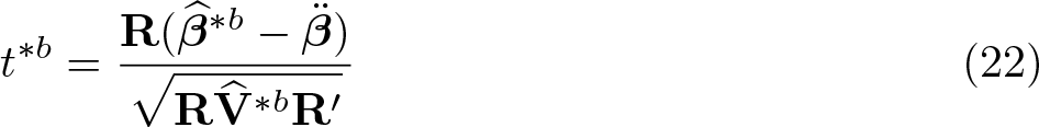
when q = 1, the t statistic in (16) is replaced by

t = \frac{R \hat{β} - r}{\sqrt{R \hat{V} R^{'}}}

with r a scalar, and the bootstrap t statistic in (17) is replaced by

t^{* b} = \frac{R ({\hat{β}}^{* b} - \ddot{β})}{\sqrt{{R \hat{V}}^{* b} R^{'}}}

For the WCR bootstrap, the numerator of (22) reduces to $R {\hat{β}}^{* b} - r$ because $R \ddot{β} = R \tilde{β} = r$ . For the WCU bootstrap, it reduces to $R ({\hat{β}}^{* b} - \hat{β})$ . In both cases, the hypothesis being tested on the bootstrap samples is true in the bootstrap DGP.

When q > 1 in (20), the t statistic (21) is replaced by the Wald statistic

W = {(R \hat{β} - R)}^{'} {(R \hat{V} R^{'})}^{- 1} (R \hat{β} - R)

and the bootstrap t statistic (22) is replaced by the bootstrap Wald statistic

W^{* b} = {R ({\hat{β}}^{* b} - \ddot{β})}^{'} {({R \hat{V}}^{* b} R^{'})}^{- 1} {R ({\hat{β}}^{* b} - \ddot{β})}

The vector that appears twice in the quadratic form (23) is the numerator of (22), and the discussion that follows that equation applies here too. We will sometimes, by a slight abuse of terminology, call this vector the Wald numerator and the matrix that is inverted in (23) the Wald denominator. Because W ≥ 0, only one type of bootstrap p-value, namely, ${\hat{P}}_{U}^{*}$ , is relevant when q > 1. Thus, the p-value for the bootstrap Wald test is simply the fraction of the W ^∗ ^b that exceed W.

3.4 The distribution of the auxiliary random variable

After (14), we noted that the auxiliary random variable $v_{g}^{* b}$ that multiplies the residual vectors ü _g in the bootstrap DGP—the “wild weight”—is usually drawn from the Rademacher distribution, taking the values −1 and +1 with equal probability. Under this distribution, $E^{*} (v_{g}^{* b}) = 0$ and $E^{*} {{(v_{g}^{* b})}^{2}} = E {{(v_{g}^{* b})}^{4}} = 1$ , so multiplying the residuals by $v_{g}^{* b}$ ensures that the first, second, and fourth moments of the residuals are preserved by the errors in the bootstrap samples. In fact, the Rademacher distribution is the only distribution that preserves first, second, and fourth moments. However, because its third moment is 0, it imposes symmetry on the distribution of the bootstrap error terms. Even if the elements of ü _g are skewed, the elements of $u_{g}^{* b}$ will not be. To that extent, the bootstrap errors become unrepresentative of the original sample errors. Unfortunately, there does not exist any auxiliary distribution that preserves all the first four moments (MacKinnon 2015, 24–25).

Other distributions that have been proposed include the following:

The Mammen (1993) two-point distribution, which takes the value 1−φ with probability φ/√5 and the value φ otherwise, where φ = (1 + √5)/2 is the golden ratio. One can confirm that, under this distribution, $E^{*} (v_{g}^{* b}) = 0$ and $E^{*} {{(v_{g}^{* b})}^{2}} = E {{(v_{g}^{* b})}^{3}} = 1$ . This means that the Mammen distribution preserves the first three moments of the residuals. Because its fourth moment is 2, it magnifies the kurtosis of the bootstrap errors. However, it does have the smallest kurtosis among all distributions with the same first three moments.

The Webb (2014) six-point distribution. As noted at the end of section 3.1, the Rademacher distribution can yield only 2 ^G distinct bootstrap samples. This is true for all two-point distributions. The six-point distribution reduces, but does not totally eliminate, this problem by assigning probability 1/6 to each of 6 points, namely, $\pm \sqrt{1 / 2}, \pm \sqrt{1 / 2} = \pm 1, and \pm \sqrt{1 / 2}$ . Its first three moments are 0, 1, and 0, like the Rademacher, so that it preserves first and second moments and also imposes symmetry on the bootstrap errors. Its fourth moment is 7/6, which enlarges kurtosis only slightly.

The standard normal distribution, for which the first four moments are 0, 1, 0, and 3. This choice allows for an infinite number of possible bootstrap samples. It preserves the first two moments, but it imposes symmetry, and the large fourth moment greatly magnifies kurtosis.

The gamma distribution with shape parameter 4 and scale parameter 1/2, as suggested by Liu (1988). Like the Mammen distribution, this has the third moment equal to 1. However, its fourth moment of 9/2 greatly enlarges kurtosis.

Simulation studies suggest that wild bootstrap tests based on the Rademacher distribution perform better than ones based on other auxiliary distributions; see Davidson, Monticini, and Peel (2007), Davidson and Flachaire (2008), and Finlay and Magnusson (2014), among others. However, the Webb six-point distribution is preferred to the Rademacher when G is less than 10 or perhaps 12. boottest offers all of these distributions and defaults to the Rademacher; see the weighttype() option in section 7.

3.5 Inverting a test to construct a confidence set

Any test of a hypothesis of the form R β = r implies a confidence set, which at level 1It−isα consists of all values of r for which P (the p-value for the test) is no less than α. easiest to see this in the case of a single linear restriction of the form β_j = β_j ₀, where β_j is the jth element of β. The confidence set then consists of all values of β_j ₀ for which the p-value for the test of β_j = β_j ₀ is equal to or greater than α.

Viewing a test as a mapping from values of β_j ₀ to p-values, we see that the confidence set is the inverse image of the interval [α, 1]. For bootstrap tests based on the algorithm of section 3.1, this mapping is given by one of the bootstrap p-values in step 5. When the bootstrap test that is inverted is based on a t statistic, as all the tests we discuss are, the resulting interval is often called a studentized bootstrap confidence interval. These intervals may be equal tailed, symmetric, or one sided, according to what type of bootstrap p-value is used to construct them.

As discussed in section 3.2, it is generally preferable to impose the null hypothesis when performing a bootstrap test. This is equally true when constructing a confidence interval. However, WCU does have a computational advantage over WCR in the latter case. For hypotheses of the form β_j = β_j ₀, inverting a bootstrap test means finding values of β_j ₀ such that the associated bootstrap p-values are equal to α. With WCU, finding these values is straightforward because, by definition, the WCU bootstrap DGP does not depend on the null hypothesis. Therefore, as we vary β_j ₀, the bootstrap samples do not change, and hence, only one set of bootstrap samples needs to be constructed. Determining the bounds of the confidence set merely requires solving (16) for β_j ₀ and plugging in the values for t_j that correspond to appropriate quantiles of the bootstrap distribution. For example, an equal-tailed studentized WCU bootstrap confidence interval is obtained by plugging in the α/2 and 1 − α/2 quantiles of the distribution of the $t_{j}^{* b}$ , while a symmetric interval is obtained by plugging in the 1 − α quantile of the distribution of the | $t_{j}^{* b}$ |.

For the WCR bootstrap, by contrast, the bootstrap samples depend on the null, so they must be recomputed for each trial value of β_j ₀. In this case, it is essential for the convergence of the algorithm that the same set of $v_{g}^{* b}$ values be used in each iteration. An iterative search in which each step requires a simulation could be computationally impractical. Fortunately, as we discuss in section 5, the WCR bootstrap can be made to run extremely fast in many applications. Moreover, the search for bounds can be implemented to minimize recomputation by precomputing all quantities in the WCR algorithm that do not depend on β_j ₀. Because boottest embodies this strategy, it can typically invert WCR bootstrap tests quickly.

By default, boottest begins the search for confidence interval bounds by picking two trial values for β_j ₀, low and high, at which P < α. boottest then calculates the pvalue at 25 evenly spaced points between these extreme bounds. From these 25 results, it selects those adjacent pairs of points between which the p-value crosses α and then finds the crossover points via an iterative search. In IV applications (section 6.1), when identification is weak, the confidence set constructed in this way may consist of more than one disjoint segment, and these segments may be unbounded; see section 8.4.

We have focused on the most common case, in which just one coefficient is restricted. However, boottest can invert any linear restriction of the form R β = r, in which R is now a 1 × k vector and r is a scalar. For example, if the restriction is that β ₂ = β ₃, R is a row vector with 1 as its second element, −1 as its third element, and every other element equal to 0. Under the null hypothesis, r = 0. In this case, the confidence set contains all values of r for which the bootstrap p-values are equal to or greater than α.

4 Multiway clustering

In section 2, we assumed that error terms for observations in different clusters are uncorrelated. In some settings, this assumption is unrealistic. In modeling panel data at the firm level, for example, one might expect correlations both within firms over time and across firms at a given time. The variance and covariance patterns are typically unknown in both dimensions. Cameron, Gelbach, and Miller (2011), hereafter CGM (2011), and Thompson (2011) separately proposed a method for constructing cluster– robust variance matrices for the coefficients of linear regression models when the error terms are clustered in two or more dimensions.⁵ The theoretical properties of the multiway CRVE were analyzed by MacKinnon, Nielsen, and Webb (2017), Menzel (2017), and Davezies, D’Haultfœuille, and Guyonvarch (2018). These articles also proposed and studied bootstrap methods for multiway clustered data.

In the next subsection, we define the multiway CRVE and discuss some practical considerations in computing it. Then, in section 4.2, we discuss how to combine multiway clustering with the wild bootstrap.

4.1 Computing the multiway CRVE

boottest allows multiway clustering along an arbitrary number of dimensions. For ease of exposition, however, we consider the two-way case. We index the G clusters in the first dimension by g and the H clusters in the second dimension by h. We attach subscripts G and H to objects previously defined for one-way clustering, such as S and Ω, to indicate which clustering dimension they are associated with. Similarly, the subscript “GH” indicates clustering by the intersection of the two primary clustering dimensions. The compound subscript “G, H” refers to the two-way clustered matrices proposed in CGM (2011) and Thompson (2011) and defined below.

The two-way CRVE extends the one-way CRVE intuitively. Recall from (6) that the one-way CRVE is built around the matrix $\hat{Ω}$ , which has i, j entry equal to ${\hat{u}}_{i} {\hat{u}}_{j}$ if observations i and j are in the same cluster and 0 otherwise. The two-way CRVE is obtained by augmenting that definition: ${\hat{Ω}}_{G, H}$ is the matrix with i, j entry equal to ${\hat{u}}_{i} {\hat{u}}_{j}$ if observations i and j are in the same G-cluster or the same H-cluster and 0 otherwise.

As a practical matter, we might try to compute ${\hat{Ω}}_{G, H} as {\hat{Ω}}_{G} + {\hat{Ω}}_{H}$ . But if observations i and j were in the same G-cluster and the same H-cluster, this would double count: entry i, j would be ${2 \hat{u}}_{i} {\hat{u}}_{j}$ . To eliminate this double counting, we instead compute

{\hat{Ω}}_{G, H} = {\hat{Ω}}_{G} + {\hat{Ω}}_{H} - {\hat{Ω}}_{G H}

Replacing $\hat{Ω}$ in (6) by ${\hat{Ω}}_{G, H}$ gives us the two-way CRVE,

{\hat{V}}_{G, H} = {\hat{V}}_{G} + {\hat{V}}_{H} - {\hat{V}}_{G H}

where we have used (24) and the linearity of (6) in $\hat{Ω}$ .

By analogy with the standard Stata small-sample correction for the one-way case given in (13), CGM (2011) suggested redefining ${\hat{V}}_{G, H}$ as follows,

{\hat{V}}_{G, H} = m_{G} {\hat{V}}_{G} + m_{H} {\hat{V}}_{H} - m_{G H} {\hat{V}}_{G H}

where the three scalar m factors are computed as in (13). The number of clusters used in computing m_GH is the number of nonempty intersections between G and H clusters, which may be less than the product G × H. CGM’s (2011) cgmreg program uses these factors, as does cgmwildboot (Caskey 2010), which is derived from cgmreg. However, another popular implementation of multiway clustering, ivreg2 (Baum, Schaffer, and Stillman 2007), takes the largest of m_G , m_H , and m_GH and uses it in place of all three. (The largest is always m_G or m_H .) This choice carries over to programs that work as wrappers around ivreg2, including weakiv (Finlay, Magnusson, and Schaffer 2014), xtivreg2 (Schaffer 2005), and reghdfe (Correia 2014).

boottest uses CGM’s (2011) choices for the m factors in (26). One reason is that this helps to address a practical issue that arises in computing the multiway CRVE. Computing the matrix ${\hat{V}}_{G, H}$ in (26) involves subtraction, so in finite samples the result is not guaranteed to be positive definite. When it is not, the Wald statistic can be negative, or the denominator of the t statistic can be the square root of a negative number. Multiplying the negative term in (26) by a smaller factor, that is, by m_GH instead of the larger of m_G and m_H , increases the chance that ${\hat{V}}_{G, H}$ is positive definite.

Nevertheless, the possibility that ${\hat{V}}_{G, H}$ is not positive definite still needs to be confronted. A fuller solution proposed in CGM (2011) starts by taking the eigendecomposition ${\hat{V}}_{G, H} = U Λ U^{'}$ ′. Then, it censors any negative eigenvalues in Λ to zero, giving Λ ⁺, and builds a positive semidefinite variance matrix estimate

{\hat{V}}_{G, H}^{+} = U Λ^{+} U^{'}

This solution, however, has some disadvantages. First, there appears to be no strong theoretical justification for (27). Second, because ${\hat{V}}_{G, H}^{+}$ is only positive semidefinite, not positive definite, it does not guarantee that Wald and t statistics will have the right properties.⁶ Third, replacing ${\hat{V}}_{G, H} by {\hat{V}}_{G, H}^{+}$ may often be unnecessary, because the relevant quantity ${R \hat{V}}_{G, H} R^{'}$ in the denominator of the test statistic can be positive definite—which is what is needed—even when ${\hat{V}}_{G, H}$ is not. Modifying ${\hat{V}}_{G, H}$ in that case may unnecessarily change the finite-sample distribution of the test statistics. Fourth, as a by-product of computational choices that dramatically increase speed, boottest never actually computes ${\hat{V}}_{G, H}$ ; see section 5. It would have to do that to compute the eigendecomposition; consequently, the computational burden of doing so would be substantial.

For these reasons, boottest does not modify ${\hat{V}}_{G, H}$ in the manner of CGM (2011). If this results in a test statistic that is invalid, the package simply reports the test to be infeasible.

Asymptotic properties of the multiway CRVE are analyzed in MacKinnon, Nielsen, and Webb (2017). That article also presents simulations that suggest that CRVE-based inference is unreliable in certain cases, including when the number of clusters in any dimension is small or the cluster sizes are very heterogeneous or both. It also discusses several methods for combining the wild and wild cluster bootstraps with the multiway CRVE, proves their asymptotic validity, and shows by simulation that they can lead to greatly improved inferences.

4.2 Wild-bootstrapping the multiway CRVE

The wild bootstrap and the multiway CRVE appear to have been combined first in the package cgmwildboot (Caskey 2010). Bringing them together raises several practical issues, in addition to those discussed in the context of the one-way wild cluster bootstrap.

The first practical issue that arises in wild-bootstrapping the multiway CRVE is what to do when some of the bootstrap variance matrices, ${\hat{V}}^{* b}$ , are not positive definite. In their simulations, MacKinnon, Nielsen, and Webb (2017) apply the CGM (2011) correction (27) to these, too. In contrast, boottest merely omits instances where the test statistic is degenerate from the bootstrap distribution and decrements the value of B accordingly.⁷ Like the CGM (2011) approach, deleting infeasible statistics from the bootstrap distribution is atheoretical. However, reassuringly, rerunning the Monte Carlo experiments of MacKinnon, Nielsen, and Webb (2017) with the CGM (2011) correction disabled suggests that the change has little effect in the cases examined in those experiments.⁸

The second practical issue is that, in contrast with the one-way case, the choice of small-sample correction factors now affects results. boottest applies CGM’s (2011) proposed values for m_G , m_H , and m_GH in (26) also to each bootstrap sample for the reasons discussed above. Because each component of (26) is scaled by a different factor, the scaling affects the actual and bootstrap CRVEs differently. Although the impact is likely minor in most cases, it might not be when at least one of G and H is very small. An alternative would be to set all three factors to max(m_G, m_H ), as ivreg2 does (or would, if it were bootstrapped). If this were done for both the actual and bootstrap CRVEs, it would be equivalent to using no small-sample correction at all.

The third issue is that the elegant symmetry of the multiway CRVE formula does not carry over naturally to the wild bootstrap. The wild cluster bootstrap is designed to preserve the pattern of correlations within each cluster for one-way clustering, but it cannot preserve the correlations in two or more dimensions at once. Therefore, we must now distinguish between the error clusterings and the bootstrap clustering. In bootstrapping, should we draw and apply one “wild weight” for each G-cluster, or for each H-cluster, or perhaps for each GH-cluster? The implementation in boottest supports all of these choices and defaults to the last of them; see the bootcluster() option in section 7.⁹ Monte Carlo experiments in MacKinnon, Nielsen, and Webb (2017) suggest that wild bootstrap tests typically perform best when the bootstrap applies clustering in the dimension with fewest clusters.

However, even this strategy fails in at least one case, namely, in treatment models where treatment occurs in only a few clusters, with or without a difference-in-differences structure. Here the WCR bootstrap can dramatically underreject and the WCU bootstrap dramatically overreject. In this context, MacKinnon and Webb (2018) proposed turning to a subcluster bootstrap, in which the bootstrap error terms are clustered more finely than the CRVE. The subcluster bootstrap of course includes the ordinary wild bootstrap as a limiting case. We demonstrate the potential of this approach in section 8.3.

5 Fast execution of the wild cluster bootstrap for OLS

It is easy to implement the one-way wild cluster bootstrap in Stata’s ado-programming language. However, this is computationally extremely inefficient. This section explains how to speed up the wild cluster bootstrap in the Stata environment. The efficiency gains make the wild cluster bootstrap feasible for datasets with millions of observations, even with a million bootstrap replications, and even when running the bootstrap test repeatedly to invert it and construct confidence sets. The main proviso is that the number of clusters for the bootstrap DGP should not be too large.

Moving from Stata’s ado-programming language to its compiled Mata language accounts for some of the gain in speed. However, when the number of clusters G is small relative to N, a much more substantial gain arises by taking advantage of linearity and the associativity of matrix multiplication to reorder operations. The wild cluster bootstrap turns out to be especially amenable to such tricks, which are explained in detail below and could be used with any programming language. The asymptotic computational complexity of using B bootstrap samples decreases from O(NB) to O(G ² B).

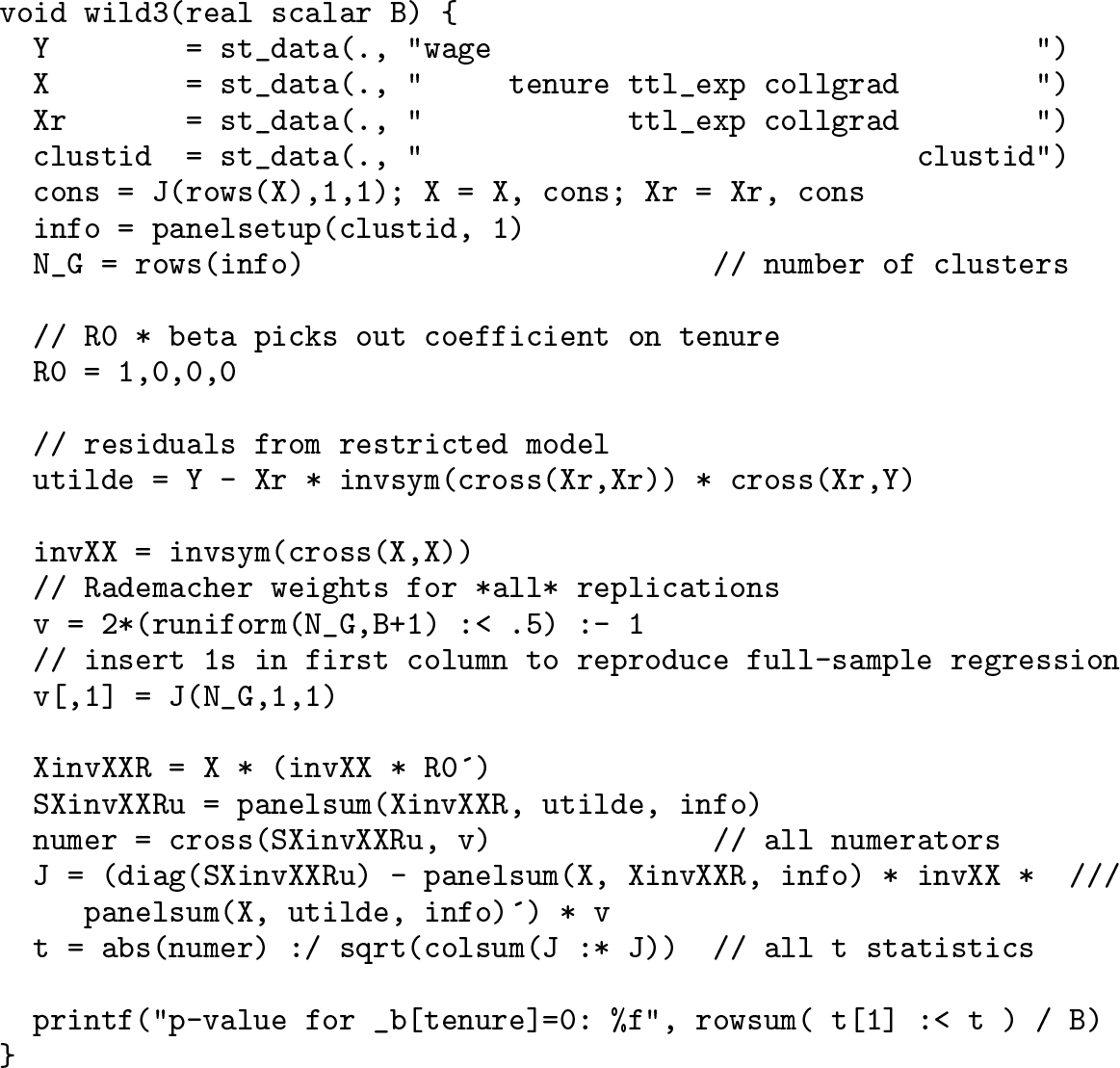
To illustrate the computational methods employed by boottest, we use Stata’s nlsw88.dta, which is an extract from the National Longitudinal Surveys of Young Women and Mature Women. We fit a linear regression model to wage(hourly wage) with covariates tenure (years in current job), ttl exp (total work experience), collgrad (a dummy for college graduates), and a constant. There are 2,217 observations, clustered into 12 industries. We test the null hypothesis that β _tenure, the coefficient on tenure, is equal to 0 against the alternative β _tenure ≠ 0

We first implement the WCR bootstrap test of this hypothesis in the ado-language, as in CGM’s (2008) bs example.do ¹⁰ and cgmwildboot. To prepare the ground, the following code sets the random-number seed (to ensure exact replicability) and loads the dataset. It then takes two steps to simplify subsequent programming: recoding the industry identifier to run sequentially from 1 to 12 in the new variable clustid and then sorting the data by this variable:

set seed 293867483

webuse nlsw88, clear

drop if industry==. | tenure==.

egen clustid = group(industry)

sort clustid, stable

The next code block applies the WCR to test β _tenure = 0. The code imposes the null on the bootstrap DGP, takes Rademacher draws, runs B = 999 replications, and computes the symmetric, two-tailed p-value, ${\hat{P}}_{S}^{*}$

One subtlety in the code warrants explanation. In the line that generates ystar, the expression “v[clustid]” exploits the ado-language’s ability to treat a variable as a vector. For each observation, the expression obtains the value of clustid, between 1 and 12, and looks up the corresponding entry in v, whose first 12 rows hold the Rademacher draws for a given replication, one for each industry cluster.

Having prepared the data and code, we run the latter on the former:

. wild1, b(999)

p-value for _b[tenure]=0: .2952953

When we run Stata 15.1 in Windows on a single core of an Intel i7-8650 in a Lenovo laptop, this bootstrap test takes 7.19 seconds.

Next, we translate the algorithm rather literally into Mata. In contrast to the adoversion, the Mata version must perform OLS and compute the CRVE itself, according to (3), (7), and (12). We will not explain every line; readers can consult the relevant Mata documentation:

A trick introduced here is to run the replication loop B + 1 times to compute the actual and bootstrap test statistics with the same code. In the first (extra) iteration, we set every element of v ^∗ to 1, which forces y ^∗ ¹ = y.

We run this Mata version of the code with B = 9999 replications:

. mata wild2(9999)

p-value for _b[tenure]=0: .290929093

Despite the tenfold increase in the number of replications, the run time falls by more than half, to 3.0 seconds. This shows how much more efficient it can be to use Mata compared with ado-based bootstrapping. To be fair, the slowness of the ado-implementation is not pure inefficiency. For example, regress computes the matrix (X′X)⁻ ¹ to estimate the parameter covariance matrix, but it does not estimate the parameters themselves via $\hat{β} = {(X' X)}^{- 1} X' y$ as in the Mata code. Rather, it solves $X' X \hat{β} = X' y$ , which is slower but more numerically stable when X is ill conditioned (Gould 2010). However, much of the work that regress does in our context is redundant, including a check for collinearity of the regressors in every bootstrap replication.

The code above is not fully optimized for Mata. We will gain further efficiency through careful analysis of the mathematical recipe. Our strategy includes these steps:

Consolidate the algorithm into a series of equations expressing the computations.

Combine steps by substituting earlier equations into later ones.

Use the linearity and associativity of matrix multiplication to reorder calculations.

Two main techniques fall under the heading of item 3:

Multiplying by thin, dimension-reducing matrices first. For example, if A is 1×100 and B and C are 100×100, computing (AB)C takes 20,000 scalar multiplications (and nearly as many additions) while A(BC) takes 1,010,000. More generally, because the final output of each replication is a scalar test statistic, constructing large, for example, N × N or N × B, matrices during the calculations is typically inefficient, because these matrices will eventually be multiplied by thin matrices to produce smaller ones. Reordering calculations can allow dimension-reducing multiplications to occur early enough so that the large matrices are never needed.

“Vectorizing” loops via built-in matrix operations. Mata programs are precompiled into universal byte code and then, at run time, translated into environmentspecific machine language. The two-step process produces code that runs more slowly than code produced in a single step by an environment-specific C or Fortran compiler. But Mata’s built-in operators, such as matrix multiplication, and some of its functions, are implemented in C or Fortran and are fully precompiled, making them very fast. In Mata, for example, matrix multiplication is hundreds of times faster when using the built-in implementation than when running explicit for loops of scalar mathematical operations. Similarly, left-multiplication by S, defined in section 2, can be performed with the fast panelsum() function added in Stata version 13.0.¹¹

We next demonstrate how to perform the above steps in the context of the wild cluster bootstrap. First, we show that when q = 1 (leaving treatment of the case with q ≥ 1 to appendix A), each wild-bootstrap Wald statistic can be written as

v^{* b}' a {(m v^{* b}' B B' v^{* b})}^{- 1} a' v^{* b}

where v ^∗ ^b is the G-vector of wild weights, a is also G × 1, and B is G × G. The small matrices a and B are fixed across replications and so only need to be computed once. With care, they can be built without creating large intermediate matrices. It is then convenient to compute all the bootstrap Wald numerators and denominators at once via a′v ^∗ and B′v ^∗, where v ^∗ is the G × B matrix with bth column equal to v ^∗ ^b .

The following equations consolidate the computations required to perform the bth bootstrap replication (all of which were presented earlier). The equations start after the OLS regression of (1), which yields the residuals ü and estimates $\ddot{β}$ :

u^{*}^{b} = ü : * S' v^{*}^{b} (bootstrap errors)

y^{* b} = X \ddot{β} + u^{* b} (bootstrap sample)

{\hat{β}}^{* b} = {(X' X)}^{- 1} X' y^{* b} (bootstrap OLS fit)

{\hat{u}}^{* b} = y^{* b} - X {\hat{β}}^{* b} (bootstrap residuals)

{\hat{V}}^{* b} = m {(X' X)}^{- 1} X' {{\hat{u}}^{* b} : * S' S : * ({\hat{u}}^{* b})'} X {(X' X)}^{- 1} (bootstrap CRVE)

W^{*}^{b} = ({\hat{β}}^{*}^{b} - \ddot{β})' R' {(R {\hat{V}}^{*}^{b} R')}^{-}^{1} R ({\hat{β}}^{*}^{b} - \ddot{β}) (bootstrap Wald statistic)

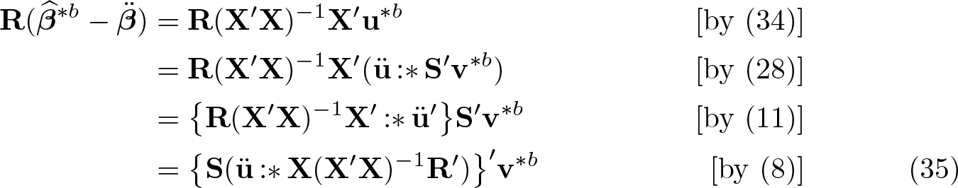
Focusing first on the Wald numerator in (33), $R ({\hat{β}}^{*}^{b} - \ddot{β})$ , observe that

{\hat{β}}^{* b} = {(X' X)}^{- 1} X' y^{* b} = {(X' X)}^{- 1} X' (X \ddot{β} + u^{* b}) = \ddot{β} + {(X' X)}^{- 1} X' u^{* b}

Thus, the numerator can be computed as

\begin{matrix} R ({\hat{β}}^{* b} - \ddot{β}) = R {(X' X)}^{- 1} X' u^{* b} [by (34)] \\ = R {(X' X)}^{-}^{1} X' (ü : * S' v^{*}^{b}) [by (28)] \\ = {R {(X' X)}^{-}^{1} X' : * ü'} S' v^{*}^{b} [by (11)] \\ = {S (ü : * X {(X' X)}^{-}^{1} R')}^{'} v^{*}^{b} [by (8)] \end{matrix}

These rearrangements flip the role of S in a way that reduces computation. The second and third lines left-multiply the vector v ^∗ ^b by S′ to expand it from height G to height N, then multiply the result by another large matrix. In contrast, the last line leftmultiplies the tall matrix ü :* X(X′X)⁻ ¹ R′ by S to collapse it from length N to length G; it does so before involving the G-vector v ^∗ ^b , the entries of which therefore need not be duplicated across observations within clusters.

Next, we vectorize (35) to compute all the bootstrap Wald numerators at once:

R ({\hat{β}}^{*} : - \ddot{β}) = {S (ü : * X {(X' X)}^{- 1} R')}^{'} v^{*}

where ${\hat{β}}^{*}$ is the k × B matrix whose columns are formed by the ${\hat{β}}^{* b}$ vectors and v ^∗ is as defined earlier. Within the factor ü :* X(X′X)⁻ ¹ R′, multiplication should proceed from right to left because R′ is thin (it is k × q, where here q = 1). Left-multiplication by the sparse matrix S is performed with the Mata panelsum() function.

Equation (36) illustrates why the computational complexity (run time) of the wild cluster bootstrap need not be O(NB). The calculations within the outer parentheses, which produce a G-vector, have to be performed only once, and their computational cost depends on N, but not B. The situation is reversed in the next step: the cost of multiplying this precomputed G-vector by the G × B matrix v ^∗ is O(GB), which of course depends on B, but not on N. Thus, provided G is not too large, it can be feasible to make B as high as 99,999 or even 999,999, regardless of sample size.

We turn now to the Wald denominator in (33). Using the identity (11) and substituting the formula for ${\hat{V}}^{*}^{b}$ in (32) into the Wald denominator in (33), we obtain

\begin{matrix} R {\hat{V}}^{*}^{b} R' = m R {(X' X)}^{-}^{1} X' {{\hat{u}}^{*}^{b} : * S' S : * ({\hat{u}}^{*}^{b})'} X {(X' X)}^{-}^{1} R' \\ = m {R {(X' X)}^{-}^{1} X' : * ({\hat{u}}^{*}^{b})'} S' S {{\hat{u}}^{*}^{b} : * X {(X' X)}^{- 1} R^{'}} \\ = m J^{*} {^{b}}^{'} J^{*}^{b} \end{matrix}

where the G × q matrix J ^∗ ^b is

J^{*}^{b} = S {{\hat{u}}^{*}^{b} : * X {(X' X)}^{- 1} R^{'}}

Again, matrix multiplications should be done from right to left.

When q = 1, the X(X′X)⁻ ¹ R′ term in (37) is a column vector, and we can vectorize (37) over all replications as

J^{*} = S {X {(X' X)}^{- 1} R^{'} : * {\hat{u}}^{*}}

{(R \hat{V} R')}^{*} = m \times colsum (J^{*} : * J^{*})

in which ${\hat{u}}^{*}$ is the N × B matrix with typical column ${\hat{u}}^{* b}$ , J ^∗ is the G × B matrix with typical column J ^∗ ^b , and, with some abuse of notation, ${(R \hat{V} R')}^{*}$ is the 1 × B vector of all the bootstrap Wald denominators.

However, this formulation is still not computationally efficient. In an intermediate step, it constructs the N × B matrix ${\hat{u}}^{*}$ , which can be impractical in large datasets. We therefore substitute the formula for ${\hat{u}}^{*}$ into (38) and reorder certain operations. Note first, using (31), (34), and (29), that

{\hat{u}}^{* b} = y^{* b} - X \ddot{β} + {{(X' X)}^{- 1} X' u^{* b}} = u^{* b} - X {(X' X)}^{- 1} X' u^{* b} = M_{X} u^{* b}

where the orthogonal projection matrix M _X = I − X(X′X)⁻ ¹ X′ yields residuals from a regression on X. Vectorizing over replications, (40) is ${\hat{u}}^{*} = M_{X} u^{*}$ Substituting this into (38), we find that

\begin{array}{l} J^{*} = S {X {(X' X)}^{-}^{1} R' : * M_{X} u^{*}} \\ = S {X {(X' X)}^{-}^{1} R' : * M_{X} (ü : * S' v^{*})} [by (28)] \\ = S {X {(X' X)}^{-}^{1} R' : * M_{X}} (ü : * S' v^{*}) [by (9)] \\ = [S {X {(X' X)}^{-}^{1} R' : * M_{X} : * ü'} S'] v^{*} [by (11)] \end{array}

The last line, like (36) for the numerator, postpones multiplication by the G × B matrix v ^∗ until everything else has been calculated.

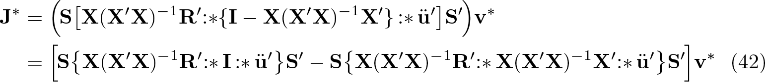
As it stands, however, (41) is still computationally expensive because M _X is an Nby×I N matrix. However, this problem is surmounted in the same way. We replace M _X − X(X′X)⁻ ¹ X′ and rearrange one last time to find that

\begin{matrix} J^{*} = (S [X {(X' X)}^{-}^{1} R' : * {I - X {(X' X)}^{-}^{1} X'} : * ü'] S') v^{*} \\ = [S {X {(X' X)}^{- 1} R' : * I : * ü'} S' - S {X {(X' X)}^{- 1} R' : * X {(X' X)}^{- 1} X' : * ü'} S'] v^{*} \end{matrix}

We can simplify the first term through the identities $S (a : * I : * b') S' = S diag (a : * b) S' = diag {S (a : * b)}$ for a and b suitably conformable column vectors. The second term can be rearranged using the identities (9) and (10). We finally obtain

J^{*} = (diag [S {X {(X' X)}^{- 1} R' : * ü}] - S {X {(X' X)}^{- 1} R' : * X} {(X' X)}^{- 1} {S (ü : * X)}') v^{*}

This formulation avoids the construction of large intermediate matrices and postpones multiplication by the G × B matrix v ^∗ until the final step.¹² Because the factor in the outer parentheses is G × G, the computational cost of multiplying it by v ^∗ is O(G ² B), whereas that for a more direct application of (38) is O(NB).

The analysis so far in this section shows that the overall computational cost of the bootstrap is O(N) + O(G ² B), where the first term is the cost of the initial calculations that are not repeated for each bootstrap sample. When G is not too large, equations (43), (39), and (36) therefore constitute an efficient algorithm for simultaneously computing the numerators and denominators for all the bootstrap test statistics.

The following Mata function applies these equations to the earlier example:

This code calls panelsum() to left-multiply by S. In doing so, it takes advantage of the function’s optional middle argument, which is a weight vector. Thus, S(ü :* X) in (43) becomes not panelsum(X:*utilde, info) but panelsum(X, utilde, info), which is equivalent but slightly faster.

Returning to our example, we run the new function:

. mata wild3(999999)

p-value for _b[tenure]=0: .290672291

The number of replications has gone up by an additional factor of 100, but the run time has dropped from 3.0 to 0.69 seconds. Compared with the original (ado) implementation, the final implementation is 10,000 times faster per replication.

Appendix A generalizes this discussion to include observation weights, one-way FEs, multiway clustering, subcluster bootstrapping, inversion of the test to form confidence sets, and higher-dimensional hypotheses (q > 1). It shows, for example, how to avoid construction of large matrices even when the model contains FEs for a grouping that is not congruent with the error clustering.

Having demonstrated how to dramatically speed up the wild cluster bootstrap, we end with a word of caution. The method can backfire when a key assumption—that there are relatively few clusters in the bootstrap DGP—is violated. For example, the G × B wild weight matrix v ^∗ can become untenably large if G is of the same order of magnitude as N. In many contexts, if G is large, the bootstrap will be unnecessary, because large-sample theory will apply and tests based on standard distributions such as the t distribution will be reliable. However, that is not always the case. For example, in multiway clustering, the last term on the right-hand side of (25) can contain a large number of clusters. Another possibility is that the number of bootstrapping clusters may greatly exceed the number of error clusters, as in the subcluster bootstrap introduced at the end of section 4.2.

boottest is also written to minimize, or at least mitigate, the computational burden when G is large. It uses specially optimized code for the extreme “robust” case, in which G = N. If the number of clusters is large yet smaller than N, it switches to a more direct implementation of (38). In either case, an issue distinct from computational burden may arise: the storage needed for the G × B matrix v ^∗ may exceed available RAM. Performance will then degrade sharply as virtual memory is cached to disk. To forestall such a slowdown, the user can invoke boottest‘s matsizegb() option, which partitions v ^∗ horizontally into chunks, creating and destroying each in turn; see section 7.

6 Extensions to IV, GMM, and ML

The tests that boottest implements are not limited to models estimated by OLS. In this section, we briefly discuss boottest implementations of the wild bootstrap in the context of other estimation methods.

6.1 The WRE bootstrap for IV estimation

Davidson and MacKinnon (2010) proposed an extension of the wild bootstrap to linear regression models estimated with IV. We consider the model

y_{1} = Y_{2} γ + X_{1} β + u_{1}

Y_{2} = X_{1} Π_{1} + X_{2} Π_{2} + U_{2}

where y ₁, Y ₂, X ₁, and X ₂ are the observation vectors or matrices for the dependent variable, the endogenous (or instrumented) variables, the included exogenous variables, and the excluded exogenous variables (instruments), respectively. Equation (44) is the structural equation for y ₁, and (45) is the reduced-form equation for Y ₂. The matrices Y ₂, Π ₁, Π ₂, and U ₂ all have one column for each endogenous variable on the right-hand side of (44).

Davidson and MacKinnon (2010) allowed for correlation between corresponding elements of u ₁ and U ₂, and for heteroskedasticity, but not for within-cluster dependence. We will instead consider the clustered case, to which Davidson and MacKinnon’s (2010) WRE bootstrap naturally extends (Finlay and Magnusson 2014). Once again, we make no assumption about the within-cluster error variances and covariances. We merely assume that, if observations i and j are in different clusters, then E(u ₁ _iu ₁ _j ), E(u ₁ _i u ₂ _j ), and E(u ₂ _i u2′j) are identically zero, where u ₁ _i is the ith element of u ₁ and u ₂ _j is the column vector made from the jth row of U ₂.

Like the WCR bootstrap, the WRE bootstrap begins by fitting the model subject to the null hypothesis, which in Davidson and MacKinnon (2010) is that γ = 0. Imposing this restriction on (44) makes OLS estimation appropriate. Davidson and MacKinnon (2010) suggested a technique for estimating the reduced form (45) that yields more efficient estimates than simply regressing Y ₂ on X ₁ and X ₂. The residual vector from the OLS fit of (44) is added as an extra regressor in (45). This explains the word “efficient” in the name of the procedure.

As implemented in boottest, the WRE bootstrap admits null restrictions other than γ = 0. It can test any linear hypothesis involving any elements of γ and β. To achieve this generalization, boottest fits the entire system using ML, subject to Rδ = r, where δ = [γ′ β′]′.¹³ Because there is only one structural equation, the ML estimates of δ are actually LIML estimates. Appendix B derives the restricted LIML estimator used by boottest. Like classical LIML, this estimator can be computed analytically, without iterative searching. Because the estimates of Π ₁ and Π ₂ are also ML estimates, they are asymptotically equivalent to the efficient ones used in Davidson and MacKinnon’s (2010) procedure.

Having obtained estimates of all coefficients under the null hypothesis—that is, $\tilde{γ}, \tilde{β}, {\tilde{Π}}_{1}$ , and ${\tilde{Π}}_{2}$ —the WRE bootstrap works in the same way as the WCR bootstrap. It next computes the restricted-fit residuals,

\begin{matrix} {\tilde{u}}_{1} = y_{1} - (Y_{2} \tilde{γ} + X_{1} \tilde{β}) \\ {\tilde{U}}_{2} = Y_{2} - (X_{1} {\tilde{Π}}_{1} + X_{2} {\tilde{Π}}_{2}) \end{matrix}

To generate each WRE bootstrap sample, these residuals are then multiplied by the wild weight vector v ^∗ ^b , which, in the standard one-way-clustered case, has one element per cluster. This preserves the conditional variances of the error terms, their correlations within clusters, and their correlations across equations. For the bth bootstrap sample, the simulated values for all endogenous variables are then constructed as follows,

y_{1}^{* b} = Y_{2}^{* b} \tilde{γ} + X_{1} \tilde{β} + u_{1}^{* b}, u_{1}^{* b} = {\tilde{u}}_{1} : * S' v^{*}^{b}

Y_{2}^{* b} = X_{1} {\tilde{Π}}_{1} + X_{2} Π e_{2} + U_{2}^{* b}, U_{2}^{* b} = U_{2} : * S' v^{*}^{b}

where it should be noted that $Y_{2}^{* b}$ is actually generated before $y_{1}^{* b}$ .

After the bootstrap datasets have been constructed, various estimators can be applied. boottest currently supports 2SLS, LIML, k-class, Fuller LIML, and generalized method of moments (GMM) estimators. Wald tests may then be performed for hypotheses about the parameters. The WRE also extends naturally to multiway clustering and the subcluster bootstrap. boottest supports all of these possibilities, except that, for GMM estimation, it does not recompute the moment-weighting matrix for each bootstrap replication.

Unfortunately, some of the techniques introduced in section 5 to speed up execution do not work for IV estimators. The problem is that the bootstrap estimators are nonlinear in v ^∗ ^b . For example, if $Z^{* b} = [Y_{2}^{* b} X_{1}]$ is the full collection of right-hand-side bootstrap data in the y ₁ ^∗ ^b equation and X = [X ₁ X ₂] is the same for the Y ₂ equation, then the 2SLS estimator is given by

{\hat{δ}}^{* b} = {(Z^{* b})' P_{X} Z^{* b}}^{-}^{1} (Z * b)' P_{X} y_{1}^{* b}

where P _X = X(X′X)⁻ ¹ X′. This estimator is nonlinear in Z ^∗ ^b , which contains $Y_{2}^{* b}$ , which is linear in v ^∗ ^b . The resulting overall nonlinearity prevents much of the reordering of operations that is possible for OLS.

This computational limitation does not apply to the Anderson–Rubin (AR) test, which is also available in boottest. To perform an AR test of the hypothesis that γ = γ ₀, we subtract Y ₂ γ ₀ from both sides of (44) and substitute for Y ₂ from (45):

\begin{matrix} y_{1} - Y_{2} γ_{0} = Y_{2} (γ - γ_{0}) + X_{1} β + u_{1} \\ = (X_{1} Π_{1} + X_{2} Π_{2} + U_{2}) (γ - γ_{0}) + X_{1} β + u_{1} \\ = X_{1} {Π_{1} (γ - γ_{0}) + β} + X_{2} Π_{2} (γ - γ_{0}) + U_{2} (γ - γ_{0}) + u_{1} \end{matrix}

If the instruments X ₂ are valid, it must be valid to apply OLS to (48), that is, to regress y ₁ − y ₂ γ ₀ on X ₂ while controlling for X ₁. If the hypothesis γ = γ ₀ is correct and the X ₂ are valid instruments, then the coefficient on X ₂ in this regression model is zero. The AR test is computed as the Wald test that the coefficient on X ₂ equals zero. It is then interpreted as a joint test of the hypothesis γ = γ ₀ and of the overidentifying restrictions that the instruments are valid. Because the test does not involve estimating any coefficients on instrumented variables and hence does not require that the rank condition (that Π ₂ has full rank) is satisfied, it is robust to instrument weakness (Baum, Schaffer, and Stillman 2007).

Note that the AR test is exact under classical assumptions because it tests rather than assumes the key condition of instrument validity. Thus, it may seem odd to bootstrap the AR test. However, we have allowed equations (44) and (45) to have error terms that may be heteroskedastic or correlated within clusters, or both. Because the AR test is not exact under these conditions, bootstrapping it should generally improve its finite-sample properties.

When the WRE bootstrap is used to estimate the distribution of an AR test statistic, it varies only the left-hand side of (48) as it constructs bootstrap samples. In particular, using (46) and (47), the bootstrap values of the left-hand side of (48) for cluster g are

y_{1 g}^{* b} - Y_{2 g}^{* b} γ_{0} = {\tilde{y}}_{1} - {\tilde{Y}}_{2} γ_{0} + ({\tilde{u}}_{1 g} - {\tilde{U}}_{2 g} γ_{0}) v_{g}^{* b}

Therefore, the WRE bootstrap of an AR test can be implemented as a WCR bootstrap test of the hypothesis that the coefficients on X ₂ are all zero in regression (48).

We stress that the AR test has a different null hypothesis than the other tests we consider. It tests not only that the coefficients on Y ₂ take certain values but also that the instruments are valid, in the sense that the overidentifying restrictions are satisfied. In consequence, its results need to be interpreted with great care, especially if the test is inverted to construct a confidence set for γ. If the test tends to reject the null for most trial values of γ, this may simply indicate that the instrument validity assumption should be rejected rather than that γ is being estimated with high precision; see Davidson and MacKinnon (2014).

6.2 The score bootstrap

The “score bootstrap” adapts the wild bootstrap to the class of extremum estimators, which includes ML and GMM. The notion of a residual, which is central to the wild bootstrap, does not carry over directly to extremum estimators in general. Instead of working with residuals, the score bootstrap works with the observation-level contributions to the scores, which are the derivatives of the objective function with respect to the parameters. Hu and Zidek (1995) and Hu and Kalbfleisch (2000) showed how to apply the pairs bootstrap to scores. Kline and Santos (2012) applied the wild bootstrap instead, producing what they dub the score bootstrap.

Consider the probit model for binary data, $y_{i} = I (Φ (x_{i} β) > 0)$ , where ϕ (·) is the cumulative standard normal distribution function. It would make no sense to apply the wild bootstrap to such a model, because the “residuals” would equal either $- Φ (x_{i} \hat{β}) or 1 - Φ (x_{i} \hat{β}),$ depending on whether the dependent variable equaled 0 or 1.

Although there is no reason to use the score bootstrap in the context of the linear regression model in section 2, it is illuminating to see how it would work. If, for estimation purposes, the error terms are assumed to be normally and independently distributed with variance σ ², then the log-likelihood contribution of observation i is

l_{i} (β, σ) = - \frac{1}{2} log (2 π σ^{2}) - \frac{1}{2 σ^{2}} {(y_{i} - x_{i} β)}^{2}

The vector of derivatives of (49) with respect to β is (y_i − x _iβ)x _i/σ ². Evaluating this at $\ddot{β}$ and summing over all observations yields the score vector

s = \frac{1}{σ^{2}} X' ü = \sum_{g = 1}^{G} s_{g}, s_{g} = \frac{1}{σ^{2}} X'_{g} ü_{g}

where s _g is the score subvector corresponding to the gth cluster. Similarly, the negative of the Hessian matrix, the matrix of second derivatives of the log likelihood for the entire sample, is −H = X′X /σ ².

Now consider the wild bootstrap Wald statistic (23), which can also be written as

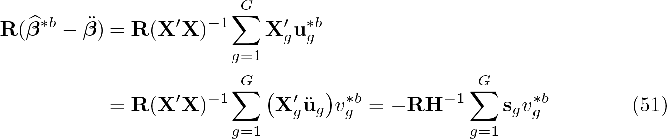
W^{* b} = ({\hat{β}}^{* b} - \ddot{β})' R' {(R {\hat{V}}^{* b} R')}^{- 1} R ({\hat{β}}^{* b} - \ddot{β})

As noted in (35), the numerator of this statistic can be rewritten as R(X′X)⁻ ¹ X′u ^∗ ^b . Therefore,

\begin{matrix} R ({\hat{β}}^{* b} - β ¨) = R {(X' X)}^{- 1} \sum_{g = 1}^{G} X_{g}^{'} u_{g}^{* b} \\ = R {(X' X)}^{- 1} \sum_{g = 1}^{G} (X_{g}' ü_{g}) v_{g}^{* b} = - R H^{- 1} \sum_{g = 1}^{G} s_{g} v_{g}^{* b} \end{matrix}

From the rightmost expression here, we see that the $v_{g}^{* b}$ are generating the bootstrap variation in the Wald numerator by perturbing the score contributions, s _g . Because of the perturbations, the full set of bootstrapped score contributions, s ^∗ ^b = X′u ^∗ ^b , is not itself a score matrix; that is, it is not a set of observation-level derivatives of any log likelihood. Nonetheless, the premise of the score bootstrap is that this randomness generates information about the distribution of the score vector from the actual sample and hence of test statistics based upon it.

In the OLS case, the score bootstrap combines the Wald numerator (51), which is the same as in the wild bootstrap, with a somewhat different estimate of its variance that avoids reference to residuals and takes scores as primary quantities. This variance estimate enters the denominator of the bootstrap Wald or score/Lagrange multiplier statistic. To show the difference, we write the wild bootstrap CRVE as

{\hat{V}}^{* b} = m {(X' X)}^{- 1} {\sum_{g = 1}^{G} X_{g}^{'} {\hat{u}}_{g}^{* b} ({\hat{u}}_{g}^{* b})' X_{g}} {(X' X)}^{-}^{1}

see (7) and (32). The score bootstrap instead uses

{\hat{V}}^{* b} = m {(X' X)}^{- 1} {\sum_{g = 1}^{G} X_{g}^{'} u_{g}^{* b} (u_{g}^{* b})' X_{g}} {(X' X)}^{-}^{1} = m H^{-}^{1} {\sum_{g = 1}^{G} s_{g}^{* b} (s_{g}^{* b})'} H^{-}^{1}

Thus the bootstrap residuals from reestimation on each bootstrap sample are dropped in favor of the bootstrap errors. The latter, when multiplied by X in the formula, constitute the bootstrap scores. In Kline and Santos (2012), s ^∗ ^b is demeaned columnwise before entering this variance estimate; see appendix A.3.

As Kline and Santos (2012) showed, this formulation generalizes straightforwardly to tests based on any extremum estimator for which cluster-level contributions to the score and the Hessian are computable. This allows us to use the computational tricks of section 5 to calculate many score bootstrap statistics quickly. When the null hypothesis is imposed, the actual test statistic that corresponds to (50) is a score or Lagrange multiplier statistic; see Wooldridge (2010, (12.68)).

The score bootstrap is computationally attractive, but it does not always provide a good approximation, for two reasons. First, as mentioned just above, in the OLS case, the denominator of the score bootstrap test statistic uses bootstrap errors instead of bootstrap residuals to calculate the variance estimate, but the test statistic that is calculated on the original data uses residuals. Hence, the distribution of the score bootstrap test statistics cannot account for the use of residuals instead of errors in the variance estimate. Second, in nonlinear models, because the scores and the Hessian for all the bootstrap samples are evaluated at $\ddot{β}$ rather than at estimates that vary across bootstrap samples, the score bootstrap cannot fully capture the nonlinearity of the estimator.

A dramatic example of the second issue can be found in Roodman and Morduch (2014), which replicated the Pitt and Khandker (1998) evaluation of microcredit programs in Bangladesh. The latter relied on a nonlinear, multiequation ML estimator, and Roodman and Morduch (2014) showed that the ML estimator was bimodal. The previously unreported second mode corresponded to negative rather than positive impact, and Wald tests performed at either mode returned large and mutually contradictory t statistics. In a pairs bootstrap, the second mode was favored in a third of the replications. Because the score bootstrap estimates test statistic distributions from the scores and Hessian computed at a single estimate, $\ddot{β}$ , it is incapable in this context of accurately representing the distribution of the parameter estimates of primary concern. We suggest that the score bootstrap not be relied upon without evidence that it works well in the case of interest.

7 The boottest package

The boottest package performs wild bootstrap tests of linear hypotheses. It is compatible with Stata versions back to 11.0, but it runs faster in Stata versions 13.0 and later because they include the Mata panelsum() function. The syntax is modeled on that of Stata’s built-in command for Wald testing, test. Like test, but unlike other Stata implementations of the wild bootstrap, boottest is a postestimation command. It determines the context for inference from the current estimation results.

The following three commands implement the extended example in section 5:

webuse nlsw88, clear

regress wage tenure ttl_exp collgrad, cluster(industry)

boottest tenure

Here, by default, boottest generates 999 wild cluster bootstrap samples using the Rademacher distribution, with the null hypothesis imposed. It reports the t statistic from the Wald test and its bootstrapped p-value (by default, symmetric). It then automatically inverts the test, as described in section 3.5, and reports the bounds of the confidence set for the default level of confidence, which is normally 95%. Finally, it plots the “confidence curve” underlying this calculation, that is, the bootstrap p-value for the hypothesis β _tenure = c as a function of c. It marks the points where the curve crosses 0.05, which are the limits of the confidence set.

In general, boottest accepts any hypothesis statement conforming to the syntax of Stata’s constraint define. The hypothesis is stated before the comma in a boottest command line, and options come after. In the hypothesis definitions, a simple reference to a regressor implies “= 0”. Similarly, the joint hypothesis β _tenure = β _ttl _exp = 0 is tested by

boottest tenure ttl_exp

Because the null hypothesis is now two dimensional, boottest also depicts the confidence surface using Stata’s twoway contour command; see figure 1. But it does not numerically describe the boundary of the confidence set that would result from intersecting this surface with the plane defined by, say, P = 0.05.

Figure 1.

p-value surface for joint hypothesis that β _tenure = β _ttl _exp = 0

Expressing more complex linear hypotheses requires the equals sign:

boottest 2*tenure + 3*ttl_exp = 4

To jointly test several complex hypotheses, we must enclose each in parentheses:

boottest (tenure) (ttl_exp = 2)

More idiosyncratically, boottest allows the user to test hypotheses independently rather than jointly, using curly braces. The following example has the same effect as running “boottest tenure” and “boottest ttl exp = 2” separately, except that it exploits the availability of the Bonferroni adjustment for multiple hypothesis testing (on which, see [R] test):

boottest {tenure} {ttl_exp = 2}, madjust(bonferroni)

Parentheses may be nested within curly braces to test several joint hypotheses separately:

boottest {(tenure) (ttl_exp=1)} {(tenure) (ttl_exp=2)}, madjust(sidak)

The boottest command can be run after application of the following estimators:

OLS, as performed by regress.

Restricted OLS, as performed by cnsreg.

Instrumental variables estimators—2SLS, LIML, Fuller’s LIML, k-class, or GMM— as fit with ivregress or the ivreg2 package of Baum, Schaffer, and Stillman (2007). In all cases, the WRE bootstrap is applied by default. boottest initializes the bootstrap DGP with LIML and, in particular, restricted LIML unless the user includes the nonull option. It then applies the user’s chosen estimator on the bootstrap datasets. After GMM estimation, boottest bootstraps only with the final moment-weighting matrix; it does not replicate the process for computing that matrix.¹⁴ By default, Wald tests are performed. However, the AR test is available; its default hypothesis is that all instrumented variables have zero coefficients and that the overidentifying restrictions are satisfied. After 2SLS and GMM, the score bootstrap is also available.

OLS and linear IV estimators with one set of “absorbed” FEs, as fit with Stata’s areg command, its xtreg and xtivreg commands with the fe option, or the community-contributed xtivreg2 (Schaffer 2005) or reghdfe (Correia 2014) command.

ML estimators, as fit with commands such as probit, logit, glm, sem, gsem, and the community-contributed cmp (Roodman 2011). Here boottest offers only the score bootstrap. To reestimate nonlinear models while imposing the null, boottest must modify and reissue the original estimation command. This requires that the estimation package accept the standard options constraints(), iterate(), and from(). The package must also support generation of scores via predict. Many ML-based estimation procedures in Stata meet these criteria. Because of the computational burden that is typical of ML estimation, boottest does not attempt to construct confidence sets by inverting score bootstrap tests.

boottest detects and accommodates the choice of variance matrix type used in the estimation procedure, be it homoskedastic, heteroskedasticity-robust, cluster–robust, or multiway cluster–robust. It does the same for small-sample corrections, such as with the small option of ivregress. It also lets users override those settings during inference, accepting its own robust, cluster(), and smalloptions. Thus, for example, tests after regress can be multiway clustered even though that command does not itself support multiway clustering. In fact, the boottest package includes the wrappers waldtest and scoretest to expose such functionality without requiring any bootstrapping. The following code shows two examples:

regress wage tenure ttl_exp collgrad, cluster(industry)

waldtest tenure, cluster(industry age)

probit c_city tenure wage ttl_exp collgrad, cluster(industry)

scoretest tenure

A third wrapper, artest, offers the nonbootstrapped AR test:

ivregress 2sls wage ttl_exp collgrad (tenure = union), cluster(industry)

artest, cluster(industry age)

The boottest command accepts the following options, nearly all of which are inherited by the wrapper commands:

nonull suppresses the imposition of the null hypothesis on the bootstrap DGP.

reps(# )sets the number of replications, B. The default is reps(999). Especially when clusters are few, increasing this number costs little in run time. reps(0) requests a Wald test or, if boottype(score) is also specified and nonull is not, a score test. The wrappers waldtest and scoretest facilitate this usage.

seed( # ) sets the initial state of the random-number generator; see [R] set seed.

ptype(symmetric| equaltail| lower| upper) chooses the p-value type from the ones listed in (18) and (19). The option applies only to unary hypotheses, ones involving a single equality. The default is ptype(symmetric) and has the p-value derived from the square of the t/z statistic or, equivalently, the absolute value. equaltail performs a two-tailed test using the t/z statistic. For example, if the confidence level is 95, then the symmetric p-value is less than 0.05 if the square of the test statistic is in the top 5 centiles of the corresponding bootstrapped distribution. The equal-tail p-value is less than 0.05 if the test statistic is in the top or bottom 2.5 centiles. In addition, lower and upper allow one-sided tests.

level(# ) specifies the confidence level, as a percentage, for the confidence interval. The default is level(95) or as set by set level. Setting it to 100 suppresses computation and plotting of the confidence set while still allowing plotting of the confidence curve or surface.

madjust(bonferroni| sidak) requests the Bonferroni or Šidák adjustment for multiple hypothesis tests. The Bonferroni p-value is min(1, nP ), where P is the unadjusted p-value and n is the number of hypotheses. The Šidák p-value is 1 − (1 − P ) ⁿ .

weighttype(rademacher| mammen| webb| normal| gamma) specifies the distribution for the wild weights, $v_{g}^{* b}$ , from among the choices in section 3.4. The default is weighttype(rademacher). For the Rademacher distribution, if the number of replications B exceeds the number of possible draw combinations, 2 ^G , then boottest will use each possible combination once (enumeration).

noci prevents the automatic computation of a confidence interval when it would otherwise be computed. This can save a lot of time when the null is imposed and when B or the number of bootstrapping clusters is large.

nograph prevents graphing of the confidence function but not the derivation of the confidence set.

small requests finite-sample corrections even after estimates that did not make them.

robust and cluster(varlist ) have the traditional meanings and override settings used in estimation. To cluster by several variables, list them all in cluster().

bootcluster(varname ) specifies the bootstrap clustering variable or variables. If more than one variable is specified, then bootstrapping is clustered by the intersections of clustering implied by the listed variables. The default is to cluster by the intersection of all the cluster()variables, although this is generally not recommended with multiway clustering; see section 4.2. Note that cluster(A B) and bootcluster(A B) mean different things. The first is two-way clustering of the errors by A and B. The second is one-way clustering of the bootstrap errors by the intersections of A and B.

ar requests the AR test. It applies only to IV estimation. The null defaults to all coefficients on endogenous (instrumented) variables being zero. If the null is specified explicitly, then it must fix all coefficients on instrumented variables, and no others.

boot type(wild| score) specifies the bootstrap type. After ML estimation, score is the default and only option. Otherwise, wild or WRE bootstrap is the default, which boottype(score) overrides in favor of the score bootstrap.

quietly, when working with ML estimates, suppresses display of the initial reestimation with the null imposed.

gridmin( # # ), gridmax( # # ), and gridpoints( # # ) override the default lower and upper bounds and the resolution of the grid search that begins the process of plotting the contour curve or surface and, for one-dimensional hypotheses, searching for the confidence interval bounds. By default, boottest estimates the lower and upper bounds by working with the bootstrap distribution. It initially evaluates 25 grid points. Reducing this number can save time in computationally demanding problems, at the cost of some crudeness in the confidence plot and the risk, if the confidence set may be disjoint, of missing one or more parts of it.

graphname( name , replace ) names any confidence plots. When multiple independent hypotheses are being tested, name will be used as a stub, producing name 1, name 2, and so on.

graphopt( string ) allows the user to pass formatting options to the graph twoway command to control the appearance of the confidence plot.

svmat (t| numer) requests that the bootstrapped test statistics be saved in return value r(dist). This can be diagnostically useful because it allows analysis of the simulated distribution. Section 8.3 below provides an example. If svmat(numer) is specified, overriding the default of svmat(t), only the test statistic numerators are returned. If the null hypothesis is that a coefficient is zero, then these numerators are the estimates of that coefficient in all the bootstrap replications.

cmdline(string) provides boottest with the command line used to generate the estimates. This is typically needed only when performing the Kline–Santos score bootstrap after estimation with the ml model command and only when imposing the null. To impose the null on an ML estimate, boottest needs to rerun the estimation subject to the constraints imposed by the null. To do that, it needs access to the command line that generated the results. Most Stata estimation commands save the command line in the e(cmdline) return macro, which boottest looks for. However, if one uses Stata’s ml model command, perhaps with a custom likelihood evaluator, no e(cmdline) is saved. The cmdline( string) option provides a work-around by allowing the user to pass the estimation command line manually.

matsizegb( # ) limits the memory demand of the G × B matrix v ^∗ to prevent caching of virtual memory to disk. The limit is specified in gigabytes. Note that this option does not limit the actual size of v ^∗. Instead, it forces boottest to break the matrix into chunks no larger than the limit, creating and destroying each chunk in turn.

8 Empirical examples

To illustrate the methods that boottest makes available, we present four empirical examples adapted from published research.

8.1 OLS with few clusters

Gruber and Poterba (1994) studied whether tax incentives prompt self-employed people to buy health insurance. They used a difference-in-differences design to study the impact of the passage of the Tax Reform Act of 1986 in the United States. The act extended a preexisting tax subsidy for employer-provided insurance to self-employed people as well. Thus, the employed served as the comparison group for the self-employed. The dataset spans the eight years 1983–1990, with the posttreatment period beginning in 1988, when the law came into full effect.

CGM (2008) revisited this study using an aggregated version of the Gruber–Poterba dataset with just 16 observations, one for each combination of year and employment type.¹⁵ They regressed the insured fraction on dummies for employment type, the posttreatment period, and the product thereof, with the last of these being the treatment dummy:

. use http://faculty.econ.ucdavis.edu/˜dlmiller/statafiles/collapsed

.regress hasinsurance selfemployed post post_self, cluster(year)

(output omitted)

This command estimates β _{post self}, the parameter of interest, to be 0.055 with a standard error of 0.0074 when clustering by year. To illustrate the wild cluster bootstrap, CGM (2008) tested the hypothesis β _{post self} = 0.04. The associated t statistic is (0.055−0.04)/0.0074 = 2.02, which, when evaluated against the standard normal and the t(6) distribution, yielded p-values of 0.043 and 0.090, respectively. They reported that a wild bootstrap with 999 replications, Mammen weights, and no imposition of the null returned P = 0.070. We obtain fairly similar results as follows:

In the first test, following Stata convention, waldtestuses the t(G−1) distribution, and here there are G = 8 clusters. For the bootstrap test, boottest produces an interesting warning. Although CGM (2008) used 999 replications, with 8 clusters, the two-point Mammen distribution can produce only 256 different bootstrap samples.

We improve on this example by imposing the null, as advised by CGM (2008) and in section 3.2, then drawing from the six-point Webb distribution, increasing the number of bootstrap samples to B = 999, 999, and inverting the test to derive a 95% confidence interval for β _{post self}:

8.2 OLS with multiway clustering

Michalopoulos and Papaioannou (2013) investigated the effect of precolonial ethnic institutions on comparative regional development in African countries. They proxied regional variation in economic activity by satellite images of light density taken at night. In section 4 of Michalopoulos and Papaioannou (2013), geographic pixels of size 0.125 × 0.125 decimal degrees are the unit of analysis. Their specification is

y_{p, i, c} = a_{c} + γ {IQL}_{i} + λ P D_{p, i, c} + Z'_{p, i, c} Ψ + X'_{i, c} Φ + ζ_{p, i, c}

where y_p,i,c represents economic activity in pixel p in the historical homeland of ethnicity i in country c. Controls include country-level FEs (a_c ), log population density (PD _p,i,c ), pixel-level variables (Z _p,i,c ), and ethnicity-country-level variables (X _i,c ). The predictor of interest is IQL _i , which represents the degree of jurisdictional hierarchy, beyond the local level, for ethnic institutions.

In the regression that we replicate—from Michalopoulos and Papaioannou (2013) table V, panel A, column 10—the dependent variable is the log of average pixel luminosity in 2007–2008. The N = 66,173 observations come from G = 49 countries and H = 94 ethno-linguistic groups. The two clustering dimensions have 295 nonempty intersections. We reproduce this regression using the Michalopoulos and Papaioannou (2013) data file¹⁶ and CGM’s (2011) multiway clustering command, cgmreg.¹⁷

The coefficient estimate of interest, for cntr tribe, is 0.156. The standard error, twoway clustered by ethno-linguistic group and country, is 0.048, yielding a t statistic (reported in Michalopoulos and Papaioannou [2013] as a z statistic) of 3.228 for the null hypothesis that γ = 0. This implies a 95% confidence interval of [0.061, 0.251].

As discussed in section 4.2, there are three natural choices for the level of bootstrap clustering in this case: by ethno-linguistic group, by country, or by the intersection of the two. Simulation results in MacKinnon, Nielsen, and Webb (2017) favor clustering in the dimension with the fewest clusters, which, in this case, is the 49 countries. For illustration, we perform tests for all three levels. Also for illustration, we move to Stata’s FE linear regression command, areg. The latter cannot perform multiway clustering, so we do not bother to specify clustering during estimation. Instead, we use the waldtest wrapper to calculate the appropriate multiway p-value. Likewise, we add the cluster() option to the boottest command lines. We then use the bootcluster() option to control the level of bootstrap clustering:

The calls to boottest return 95% confidence intervals of [0.055, 0.249], [0.045, 0.264], and [0.054, 0.249], respectively. These differ only slightly from the original [0.061, 0.251]. This is not surprising, because even the coarsest clustering dimension here contains 49 clusters. The number of clusters is probably large enough that the performance of nonbootstrap tests and confidence intervals is close to their asymptotic behavior.

8.3 Difference-in-differences with few treated clusters

Conley and Taber (2011) observed that, in difference-in-differences estimation with few treated clusters, the cluster–robust CRVE can be severely biased. In response, Conley and Taber (2011) proposed a particular application of randomization inference. MacKinnon and Webb (2017b) showed that the wild cluster bootstrap also fails in this setting: the WCU bootstrap overrejects, and the WCR bootstrap underrejects. Later, MacKinnon and Webb (2018) proposed the subcluster bootstrap mentioned in section 4.2 as a way to reduce the extent of the problem. We illustrate these findings in the context of an empirical example studied in Conley and Taber (2011).

Conley and Taber (2011) studied the impact on college enrollment of state-level merit scholarship programs using data from Current Population Surveys for all states and the District of Columbia, covering 1989–2000.¹⁸ During the study period, 10 states adopted such programs. Conley and Taber (2011) regressed an individual-level dummy for eventual college enrollment on dummies for sex, race, state, and year, as well as the treatment variable, which is a dummy for the availability of state-level scholarships. One of Conley and Taber’s (2011) specifications evaluates the average impact of all 10 states’ programs, and another focuses on the most famous program, Georgia’s HOPE, by dropping the other 9 treatment states from the sample. In both cases, standard errors are clustered by state. If G ₁ denotes the number of clusters in which treatment occurs, these models have N = 42,161, G = 51, and G ₁ = 10 for the merit scholarship regressions and N = 34,902, G = 42, and G ₁ = 1 for the HOPE scholarship regressions. Thus, the HOPE regressions illustrate the extreme case in which there is just one treated cluster.

We first consider the model with 10 states. We apply six variants of the wild cluster bootstrap to test the hypothesis that the scholarship programs were not associated with college enrollment. Three impose the null hypothesis, and three do not. Within each triplet, the first variant clusters the bootstrap errors by state, the level at which they are clustered in the CRVE. The second variant clusters the bootstrap errors by state-year combination, and the third variant clusters them by individual. Clustering by individual means not clustering at all, so this variant is actually the ordinary wild bootstrap.

The last two commands are especially demanding: memory usage temporarily rises by about 4.5GB. The primary cause is the construction of a wild weight matrix v ^∗ with one row for each of the 42,161 observations (“clusters” for bootstrapping purposes) and one column for each of the 9,999 replications.¹⁹ When the null hypothesis is imposed, the computational burden of constructing and multiplying the large matrices is compounded by the search for confidence interval bounds, which requires rerunning the bootstrap for many trial values (see section 3.5). The gridpoints(10) options save a bit of time by instructing boottest to evaluate 10 instead of the default 25 evenly spaced values in its initial search for confidence interval bounds. The cost of that choice is that the confidence curve plots, which we do not look at here, are rougher. On the hardware referenced in section 5, the penultimate command takes 9.7 minutes.²⁰

We next run the same tests for Georgia’s HOPE program alone. This time, we condense the boottest commands into a loop and take advantage of boottest‘s svmat option to save the t statistics from each bootstrap sample. To give insight into the behavior of the wild cluster bootstrap here, we plot histograms for all six distributions:

Table 1 presents parameter estimates, cluster–robust standard errors, and t statistics for the 10-state and Georgia-specific regressions, along with six bootstrap p-values and the associated 95% confidence intervals.²¹ For the 10-state regression, the p-values and confidence intervals are similar to one another, which is to be expected given the number of clusters (51) and number of treated clusters (10). In contrast, the Georgiaonly p-values and confidence intervals vary radically. As predicted by the theory in MacKinnon and Webb (2017b, 2018), the WCU bootstrap test strongly rejects and the WCR bootstrap test does not reject when the bootstrap errors are clustered by state. Clustering the bootstrap errors by state-year intersections instead of by state reduces, but does not eliminate, the disagreement. However, “clustering” the bootstrap errors by individual (that is, using the ordinary wild bootstrap) brings the restricted and unrestricted bootstrap tests into very good agreement, with almost identical p-values and confidence intervals.

Table 1.

Estimates, p-values, and 95% confidence intervals for scholarship programs

Treatment group		10 states		Georgia only
Estimate		0.0337		0.0722
Cluster–robust standard error		0.0127		0.0108
t statistic		2.664		6.713
p-values and confidence intervals:	p-val.	Conf. int.	p-val.	Conf. int.
t(G − 1)	0.010	[0.008, 0.059]	0.000	[0.050, 0.094]
Bootstrap by state, restricted	0.020	[0.007, 0.067]	0.495	[−2.787, 1.307]
Bootstrap by state, unrestricted	0.025	[0.005, 0.063]	0.000	[0.050, 0.095]
Bootstrap by state-year, restricted	0.037	[0.003, 0.066]	0.291	[−5.375, 4.700]
Bootstrap by state-year, unrestricted	0.041	[0.002, 0.066]	0.094	[−0.013, 0.157]
Bootstrap by individual, restricted	0.031	[0.004, 0.064]	0.390	[−0.099, 0.246]
Bootstrap by individual, unrestricted	0.033	[0.003, 0.064]	0.392	[−0.096, 0.240]

The simulated distributions for the six Georgia-specific bootstrap t statistics are displayed in figure 2. In all six plots, a vertical line marks the actual t statistic of 6.713. In the two leftmost panels, we see the degenerate behavior of the bootstrap distribution with clustering at the state level: it is bimodal when the null is imposed (WCR) and unimodal and narrow when it is not imposed (WCU). Bootstrapping with finer clustering produces much more plausible-looking distributions. They suggest that it would not be unusual to obtain a t statistic as large as 6.713 even if the HOPE program had no impact.

Figure 2.

Wild bootstrap distributions of t statistic in Conley and Taber (2011) difference-in-differences evaluation of Georgia’s HOPE program, varying the bootstrap clustering and whether the null is imposed

8.4 IV estimation

Levitt (1996) studied the short-term elasticity of the crime rate with respect to the incarceration rate in a U.S. state panel covering 1973–1993. To identify causal impacts, the study instrumented prisoners per capita with a set of dummies representing the somewhat arbitrarily timed progression of lawsuits over prison overcrowding. For example, if a court temporarily took control of a prison system, prison growth tended to slow at the onset of control and accelerate after control ended.

The definition of the overcrowding-lawsuit IVs is complex, so we will omit most details here. Levitt (1996) divided the life cycle of an overcrowding lawsuit into six stages and subdivided these into three substages. Starting from a dataset provided by Steven Levitt, which may not exactly match that used in the study, we computed and added these variables. We also precomputed some per-capita variables and logarithms thereof.²²

Separately for violent and property crime, Levitt regressed year-on-year log changes (D.lViolentpop and D.lPropertypop in our regressions) on the previous year’s log change in prisoners per capita (LD.lpris totpop). In the 2SLS regressions, the latter is instrumented with interactions of stage and substage as factor variables. State-level demographic and economic controls, all first-differenced, include log income per capita, unemployment, log police per capita, the metropolitan population fraction, the fraction that is black, and various age group fractions. Year and state dummies are included in the specification we copy here. Standard errors are robust to heteroskedasticity only.

This code produces our best replications of the original regressions and runs some bootstrap tests:

From ivregress, we obtain elasticity estimates of −0.456 (standard error 0.170) for violent crime and −0.243 (0.106) for property crime, as opposed to −0.379 (0.180) and −of0.261 (0.117) in Levitt (1996, table VI, cols. 3 and 6). For a more extensive discussion this study, see Roodman (2017).

The boottest command line above treats the specification in a more modern way. It two-way clusters the standard errors by state and year and then bootstraps the distribution of the resulting t statistic using the WRE (see section 6.1). It computes the equal-tail p-value, which is recommended for IV applications, in which bias toward the OLS estimate tends to make the confidence curve asymmetric (Davidson and MacKinnon 2010). The bootstrap is clustered by the coarsest error-clustering dimension, which is the year. Surprisingly, this procedure produces 95% confidence sets that are disjoint and unbounded. The confidence set for violent crime is (−∞, 0.178] ∪ [0.561, +∞) and that for property crime is (−∞, −1.546] ∪ [−0.681, 0.148] ∪ [0.407, +∞).

The confidence plots presented in figure 3 show exactly how these confidence sets were obtained.²³ The boottest command line above customizes their appearance using “gridmin(2) gridmax(2)” to set their horizontal bounds and graphopt() to pass options to the underlying graph command. For violent crime, only the interval between 0.178 and 0.561 does not belong to the 95% confidence set, because the bootstrap pvalues are less than 0.05 only in that interval. Similarly, for property crime, only the two intervals between −1.546 and −0.681 and between 0.148 and 0.407 do not belong to the 95% confidence set. These types of confidence sets may seem odd, but they can arise when the instruments are weak; see Dufour (1997).

Figure 3.

Confidence curve for short-term elasticity of violent and property crime rate with respect to imprisonment rate, using a Wald test with the WRE bootstrap, in the context of Levitt (1996) FEs IV regressions

9 Conclusion

We have discussed in detail the package boottest, which calculates several versions of the wild bootstrap for tests of linear restrictions on linear regression models with heteroskedastic errors, one-way clustering, or multiway clustering. The package also calculates the WRE bootstrap (Davidson and MacKinnon 2010) for models with one or more endogenous explanatory variables, with or without clustering, and the score bootstrap (Kline and Santos 2012) for a variety of nonlinear models.

The mathematical structure of the wild cluster bootstrap, especially for models fit by OLS, lends itself to efficient implementation, thus removing computational cost as a barrier to use. As we explained in section 5, boottest takes advantage of this, and the code is remarkably fast, even when both the number of observations and the number of bootstrap replications are very large.

The empirical examples of section 8 reinforce a well-known message from simulation studies (for example, Cameron, Gelbach, and Miller [2008]; Davidson and MacKinnon [2010]; Finlay and Magnusson [2014]; Djogbenou, MacKinnon, and Nielsen [2018]): results from wild bootstrap tests are often very similar to those from tests relying on large-sample theory, but not always. In particular, when the assumptions of asymptotic theory are far from being satisfied—for example, when there are few clusters, very unbalanced clusters, few treated clusters, or weak instruments—the bootstrap-based tests and the tests based on large-sample theory may lead to very different inferences. In these cases, indeed in almost all cases, it is preferable to rely on bootstrap-based tests because they typically exhibit better finite-sample properties.

Supplemental Material

Supplemental Material, st0549 - Fast and wild: Bootstrap inference in Stata using boottest

Supplemental Material, st0549 for Fast and wild: Bootstrap inference in Stata using boottest by David Roodman, Morten Ørregaard Nielsen, James G. MacKinnon, and Matthew D. Webb in The Stata Journal

Footnotes

10 Acknowledgments

We thank an anonymous reviewer and members of the audience at the 2018 Canadian Stata Conference for helpful comments and Joshua Roxborough for research assistance. MacKinnon and Webb thank the Social Sciences and Humanities Research Council of Canada for financial support. Nielsen thanks the Canada Research Chairs program, the Social Sciences and Humanities Research Council, and the Center for Research in Econometric Analysis of Time Series (CREATES, funded by the Danish National Research Foundation, DNRF78) for financial support.

Notes

References

Baum

C. F.

Schaffer

M. E.

Stillman

2007. Enhanced routines for instrumental variables/generalized method of moments estimation and testing. Stata Journal 7: 465–506.

Beran

1986. Discussion: Jackknife, bootstrap and other resampling methods in regression analysis. Annals of Statistics 14: 1295–1298.

Bertrand

Duflo

Mullainathan

2004. How much should we trust differences-in-differences estimates? Quarterly Journal of Economics 119: 249–275.

Bester

C. A.

Conley

T. G.

Hansen

C. B.

2011. Inference with dependent data using cluster covariance estimators. Journal of Econometrics 165: 137–151.

Cameron

A. C.

Gelbach

J. B.

Miller

D. L.

2008. Bootstrap-based improvements for inference with clustered errors. Review of Economics and Statistics 90: 414–427.

Cameron

A. C.

Gelbach

J. B.

Miller

D. L.

2011. Robust inference with multiway clustering. Journal of Business and Economic Statistics 29: 238–249.

Carter

A. V.

Schnepel

K. T.

Steigerwald

D. G.

2017. Asymptotic behavior of a t-test robust to cluster heterogeneity. Review of Economics and Statistics 99: 698–709.

Caskey

2010. cgmwildboot. https://sites.google.com/site/judsoncaskey/data.

Conley

T. G.

Taber

C. R.

2011. Inference with “difference in differences” with a small number of policy changes. Review of Economics and Statistics 93: 113–125.

10.

Correia

2014. reghdfe: Stata module to perform linear or instrumental-variable regression absorbing any number of high-dimensional fixed effects. Statistical Software Components S457874, Department of Economics, Boston College. https://ideas.repec.org/c/boc/bocode/s457874.html.

11.

Davezies

D’Haultfœuille

Guyonvarch

2018. Asymptotic results under multiway clustering. ArXiv Working Paper No. arXiv:1807.07925. https://arxiv.org/abs/1807.07925.

12.

Davidson

Monticini

Peel

2007. Implementing the wild bootstrap using a two-point distribution. Economics Letters 96: 309–315.

13.

Davidson

Flachaire

2008. The wild bootstrap, tamed at last. Journal of Econometrics 146: 162–169.

14.

Davidson

MacKinnon

J. G.

1993. Estimation and Inference in Econometrics. New York: Oxford University Press.

15.

Davidson

MacKinnon

J. G.

1999. The size distortion of bootstrap tests. Econometric Theory 15: 361–376.

16.

Davidson

MacKinnon

J. G.

2004. Econometric Theory and Methods. New York: Oxford University Press.

17.

Davidson

MacKinnon

J. G.

2010. Wild bootstrap tests for IV regression. Journal of Business and Economic Statistics 28: 128–144.

18.

Davidson

MacKinnon

J. G.

2014. Confidence sets based on inverting Anderson–Rubin tests. Econometrics Journal 17: S39–S58.

19.

Davison

A. C.

Hinkley

D. V.

1997. Bootstrap Methods and Their Application. Cambridge: Cambridge University Press.

20.

Djogbenou

A. A.

MacKinnon

J. G.

Nielsen

M. Ø.

2018. Asymptotic theory and wild bootstrap inference with clustered errors. Queen’s University, Department of Economics, Working Paper No. 1399. https://ideas.repec.org/p/qed/wpaper/1399.html.

21.

Dufour

J.-M.

1997. Some impossibility theorems in econometrics with applications to structural and dynamic models. Econometrica 65: 1365–1387.

22.

Eicker

1963. Asymptotic normality and consistency of the least squares estimators for families of linear regressions. Annals of Mathematical Statistics 34: 447–456.

23.

Field

C. A.

Welsh

A. H.

2007. Bootstrapping clustered data. Journal of the Royal Statistical Society, Series B 69: 369–390.

24.

Finlay

Magnusson

L. M.

2014. Bootstrap methods for inference with clustersample IV models. University of Western Australia, Department of Economics, Working Paper No. 14-12. https://ideas.repec.org/p/uwa/wpaper/14-12.html.

25.

Finlay

Magnusson

L. M.

Schaffer

M. E.

2014. weakiv: Stata module to perform weak-instrument-robust tests and confidencce intervals for instrumental-variable (IV) estimation of linear, probit and tobit models. Statistical Software Components S457684, Department of Economics, Boston College. https://ideas.repec.org/c/boc/bocode/s457684.html.

26.

Gould

2010. Mata Matters: Stata in Mata. Stata Journal 10: 125–142.

27.

Gruber

Poterba

1994. Tax incentives and the decision to purchase health insurance: Evidence from the self-employed. Quarterly Journal of Economics 109: 701–733.

28.

Hansen

C. B.

2007. Asymptotic properties of a robust variance matrix estimator for panel data when T is large. Journal of Econometrics 141: 597–620.

29.

Härdle

Mammen

1993. Comparing nonparametric versus parametric regression fits. Annals of Statistics 21: 1926–1947.

30.

Kalbfleisch

J. D.

2000. The estimating function bootstrap. Canadian Journal of Statistics 28: 449–481.

31.

Zidek

J. V.

1995. A bootstrap based on the estimating equations of the linear model. Biometrika 82: 263–275.

32.

Kline

Santos

2012. A score based approach to wild bootstrap inference. Journal of Econometric Methods 1: 23–41.

33.

Lee

C. H.

Steigerwald

D. G.

2018. Inference for clustered data. Stata Journal 18: 447–460.

34.

Levitt

S. D.

1996. The effect of prison population size on crime rates: Evidence from prison overcrowding litigation. Quarterly Journal of Economics 111: 319–351.

35.

Liang

K.-Y.

Zeger

S. L.

1986. Longitudinal data analysis using generalized linear models. Biometrika 73: 13–22.

36.

Liu

R. Y.

1988. Bootstrap procedures under some non-I.I.D. models. Annals of Statistics 16: 1696–1708.

37.

MacKinnon

J. G.

2009. Bootstrap hypothesis testing. In Handbook of Computational Econometrics, ed. Belsley

D. A.

Kontoghiorghes

E. J.

, 183–213. Chichester, UK: Wiley.

38.

MacKinnon

J. G.

2013. Thirty years of heteroskedasticity-robust inference. In Recent Advances and Future Directions in Causality, Prediction, and Specification Analysis: Essays in Honor of Halbert L. White Jr., ed. Chen

Swanson

N. R.

, 437–461. New York: Springer.

39.

MacKinnon

J. G.

2015. Wild cluster bootstrap confidence intervals. L’Actualité Économique 91: 11–33.

40.

MacKinnon

J. G.

Nielsen

M. Ø.

Webb

M. D.

2017. Bootstrap and asymptotic inference with multiway clustering. Queen’s University, Department of Economics, Working Paper No. 1386. https://ideas.repec.org/p/qed/wpaper/1386.html.

41.

MacKinnon

J. G.

Webb

M. D.

2017a. Pitfalls when estimating treatment effects using clustered data. Political Methodologist 24: 20–31.

42.

MacKinnon

J. G.

Webb

M. D.

2017b. Wild bootstrap inference for wildly different cluster sizes. Journal of Applied Econometrics 32: 233–254.

43.

MacKinnon

J. G.

Webb

M. D.

2018. The wild bootstrap for few (treated) clusters. Econometrics Journal 21: 114–135.

44.

Mammen

1993. Bootstrap and wild bootstrap for high dimensional linear models. Annals of Statistics 21: 255–285.

45.

Menzel

2017. Bootstrap with clustering in two or more dimensions. ArXiv Working Paper No. arXiv:1703.03043. https://arxiv.org/abs/1703.03043.

46.

Michalopoulos

Papaioannou

2013. Pre-colonial ethnic institutions and contemporary African development. Econometrica 81: 113–152.

47.

Pitt

M. M.

Khandker

S. R.

1998. The impact of group-based credit programs on poor households in Bangladesh: Does the gender of participants matter? Journal of Political Economy 106: 958–996.

48.

Roodman

2011. Fitting fully observed recursive mixed-process models with cmp. Stata Journal 11: 159–206.

49.

Roodman

2017. The impacts of incarceration on crime. Open Philanthropy Project, Working Paper. https://www.openphilanthropy.org/blog/impact-incarceration-crime.

50.

Roodman

Morduch

2014. The impact of microcredit on the poor in Bangladesh: Revisiting the evidence. Journal of Development Studies 50: 583–604.

51.

Schaffer

M. E.

2005. xtivreg2: Stata module to perform extended IV/2SLS, GMM and AC/HAC, LIML, and k-class regression for panel-data models. Statistical Software Components S456501, Department of Economics, Boston College. https://ideas.repec.org/c/boc/bocode/s456501.html.

52.

Stock

J. H.

Watson

M. W.

2008. Heteroskedasticity-robust standard errors for fixed effects panel data regression. Econometrica 76: 155–174.

53.

Thompson

S. B.

2011. Simple formulas for standard errors that cluster by both firm and time. Journal of Financial Economics 99: 1–10.

54.

Webb

M. D.

2014. Reworking wild bootstrap based inference for clustered errors. Queen’s University, Department of Economics, Working Paper No. 1315. https://ideas.repec.org/p/qed/wpaper/1315.html.

55.

White

1980. A heteroskedasticity-consistent covariance matrix estimator and a direct test for heteroskedasticity. Econometrica 48: 817–838.

56.

White

1984. Asymptotic Theory for Econometricians. London: Academic Press.

57.

Wooldridge

J. M.

2010. Econometric Analysis of Cross Section and Panel Data. 2nd ed. Cambridge, MA: MIT Press.

58.

C. F. J.

1986. Jackknife, bootstrap and other resampling methods in regression analysis. Annals of Statistics 14: 1261–1295.

Supplementary Material

Please find the following supplemental material available below.

For Open Access articles published under a Creative Commons License, all supplemental material carries the same license as the article it is associated with.

For non-Open Access articles published, all supplemental material carries a non-exclusive license, and permission requests for re-use of supplemental material or any part of supplemental material shall be sent directly to the copyright owner as specified in the copyright notice associated with the article.

0.00 MB