
Abstract
Vector autoregression (VAR) estimation is a vital tool in economic studies. VARs, however, can be dimensionally cumbersome and overparameterized. The
Keywords
1 Introduction
Since Sims (1980) popularized it, the vector autoregression (VAR) model has proven to be one of the most successful models for analyzing economic (and noneconomic) time-series data, offering descriptive analysis of the dynamics, forecasting, structural inference, and policy analysis. However, because a many-variables, higher-order VAR tends to be overparameterized—yielding weak inference—a general-to-specific (GETS) approach has been suggested to improve the inference after VAR (Campos, Ericsson, and Hendry 2005). Moreover, Asali, Abu-Qarn, and Beenstock (2017) provided additional estimators of long-run (LR) and steady-state effects that can be calculated after the VAR or the GETS VAR. Asali and Gurashvili (Forthcoming) use this framework to study the relationship between discrimination in the labor market and the macroeconomy.
To facilitate this type of analysis, from estimating the original balanced VAR to its parsimonious GETS version, and inference after each model, I developed the command
Jaeger and Paserman (2008) (henceforth, JP) used the VAR framework to analyze the cycle of violence in the Israeli–Palestinian conflict. Asali, Abu-Qarn, and Beenstock (2017) (henceforth, AAB), using the same JP data, but devising the use of GETS specifications, and offering new steady-state estimators (like the LR kill ratio or the CIR), overturned previous findings. In this article, I use the JP and AAB studies as examples of applying the
2 Statistical background: VAR, GETS VAR, Granger causality, and LR effects
To illustrate the method and test statistics, we use the simplest two-variables VAR system
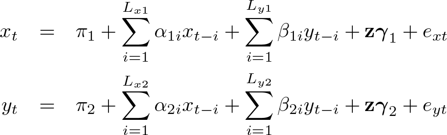
where
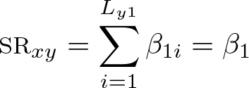
Likewise, we can define α
1
, α
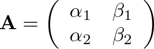
2, and β
2. These effects are grouped in the matrix
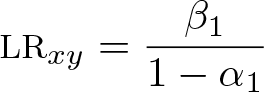
The LR effects of one variable on the other is calculated by solving that dependent variable’s equation for the LR ratios between the variables—all the SR lags being summed up over all the lags. The LR effect of y on x from the first equation (which is the LR x/y ratio) is given by
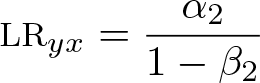
Likewise, the LR y/x ratio from the second equation is given by
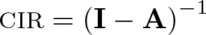
Finally, the CIR is defined as the relevant element in the matrix:
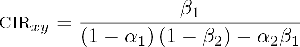
For the 2 × 2 case above, for example, the CIR of y in the x equation is given by
Statistical inference is then carried out for the effects in question (SR, LR, and CIR): the standard errors of these estimates are calculated using the delta method.
The extension to higher-order VARs is straightforward. While estimates of the LR and CIR effects are always provided for any n-variable VAR, statistical inference is limited to up-to-four-variables VAR systems because calculating the standard errors for the different CIR elements in many-variables (≥ 5) VARs is computationally prohibitive.
3 Automatic inference after VAR: vgets
The above steps can, in principle, be applied manually, but that is extremely time consuming and tedious, and the process is prone to many subtle errors of execution that are difficult to discover or fix retroactively. The command
3.1 Syntax
3.2 Description
While the point estimates of the effects are reported for any set of main variables, statistical inference (that is, robust standard errors and p-values) is calculated and reported only for systems of two, three, or four variables.
3.3 Options
3.4 Stored results
The command stores the results in
Similarly, the effects, their standard errors, and their p-values for the LR effects and the CIRs will be stored under the scalars
3.5 Example
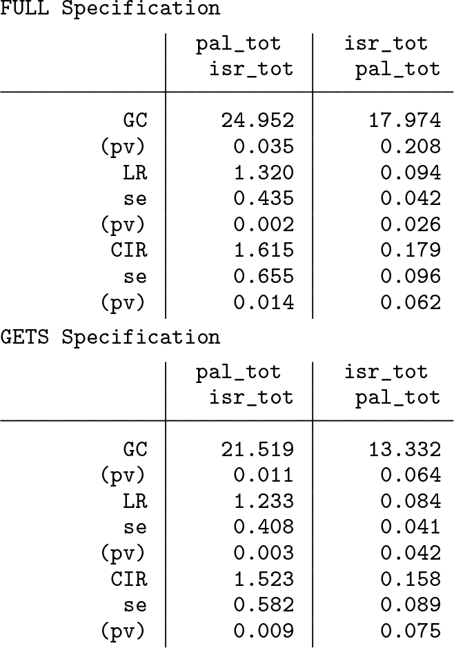
JP provided an interesting use of balanced VARs to study the cycle of violence in the Middle East. Their conclusion, regarding the absence of a cycle, however, has been overturned in AAB, who suggested the use of GETS VAR because of the overparameterization in the full, balanced specification. 1 In the Israeli–Palestinian conflict, the number of Palestinian and Israeli fatalities in day t are, respectively, pal t and isr t. The full specification of the system is given by
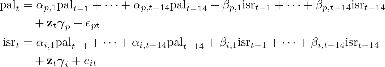
where
The first equation of the VAR is called the “Israeli reaction function”, and the second equation is called the “Palestinian reaction function”. Israel “reacts to violence” if the lags of Israeli fatalities in the Israeli reaction function Granger-cause Palestinian fatalities. Likewise, the Palestinian reaction is defined from the second equation.
The main findings of JP and AAB can be easily replicated with the
To see the underlying regressions and statistical tests, add the option
Finally,
Adding the option
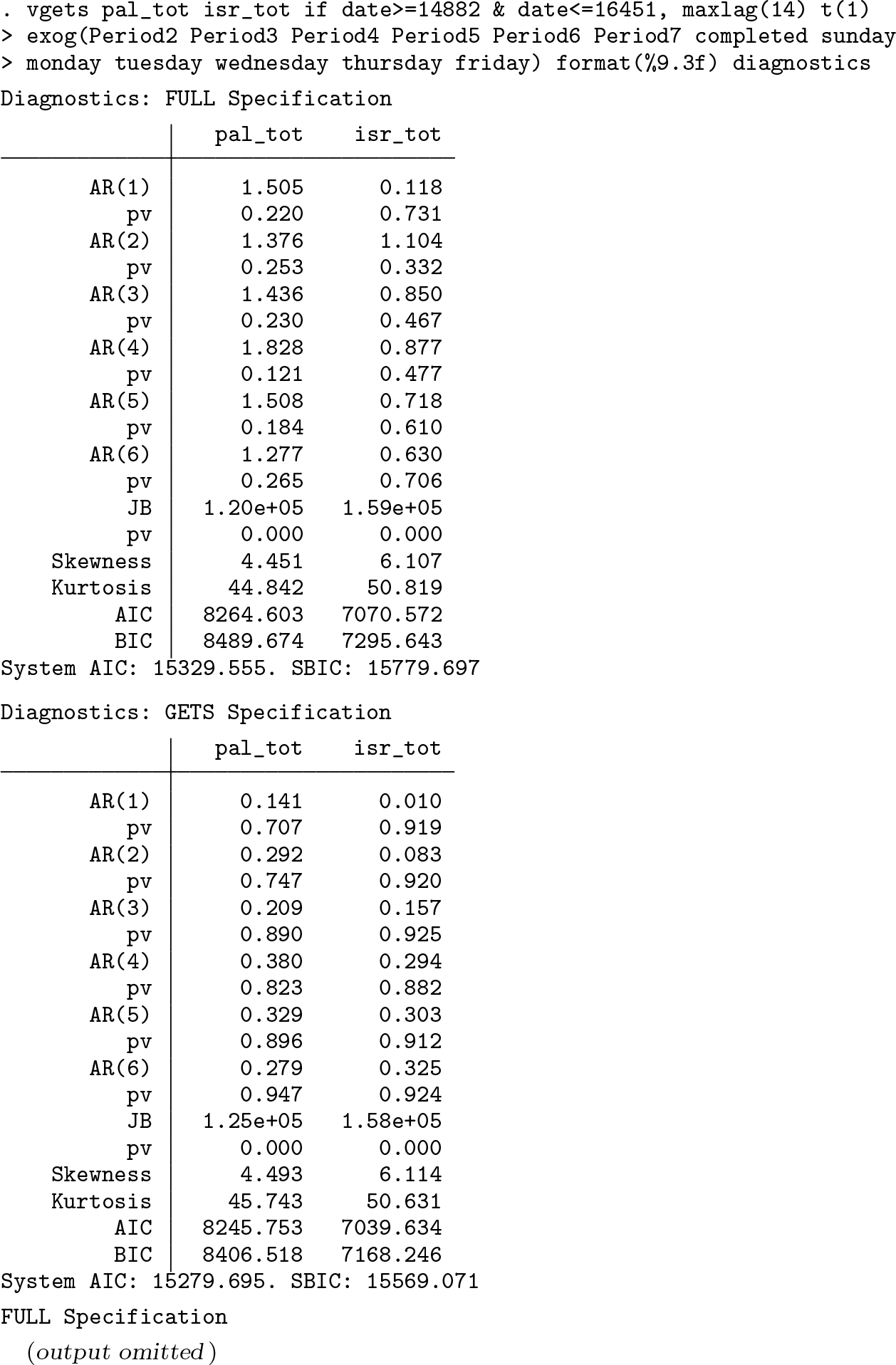
The absence of serial correlation in the residuals of the first equation, the long specification of the Israeli reaction function, renders the lagged variables weakly exogenous and therefore suggests that the Granger causality (from own Israeli fatalities to Palestinian fatalities) that we found earlier (χ 2 = 24.95, p-value = 0.035) can be interpreted as genuine causality. The same can be said about the Palestinian reaction function.
4 Conclusion
The VAR model has proven to be a useful and successful model for describing the dynamics of time-series data, offering accurate forecasting and structural inference and providing solid grounds for policy analysis. Nonetheless, the literature has argued for more parsimonious and thus more accurate specifications that do not suffer from overparameterization by applying the theory of reduction (Campos, Ericsson, and Hendry 2005). AAB have shown that using a GETS approach to the VAR analysis is important, leading not only to more accurate inference but also to actually overturning findings that are based on the fully specified VAR.
The command
5 Programs and supplemental materials
Supplemental Material, st0602 - vgets: A command to estimate general-to-specific VARs, Granger causality, steady-state effects, and cumulative impulse–responses
Supplemental Material, st0602 for vgets: A command to estimate general-to-specific VARs, Granger causality, steady-state effects, and cumulative impulse–responses by Muhammad Asali in The Stata Journal
Footnotes
5 Programs and supplemental materials
To install a snapshot of the corresponding software files as they existed at the time of publication of this article, type
Notes
References
Supplementary Material
Please find the following supplemental material available below.
For Open Access articles published under a Creative Commons License, all supplemental material carries the same license as the article it is associated with.
For non-Open Access articles published, all supplemental material carries a non-exclusive license, and permission requests for re-use of supplemental material or any part of supplemental material shall be sent directly to the copyright owner as specified in the copyright notice associated with the article.