Estimation of pre- and posttreatment average treatment effects with binary time-varying treatment using Stata

Abstract

In this article, we describe tvdiff, a community-contributed command that implements a generalization of the difference-in-differences estimator to the case of binary time-varying treatment with pre- and postintervention periods. tvdiff is flexible and can accommodate many actual situations, enabling the user to specify the number of pre- and postintervention periods and a graphical representation of the estimated coefficients. In addition, tvdiff provides two distinct tests for the necessary condition of the identification of causal effects, namely, two tests for the so-called parallel-trend assumption. tvdiff is intended to simplify applied works on program evaluation and causal inference when longitudinal data are available.

1 Introduction

In this article, we present the community-contributed command tvdiff, which implements a generalization of the difference-in-differences (DID) estimator to the case of (many) pre- and postintervention periods. tvdiff estimates average treatment effects (ATEs) when the treatment variable is binary and varying over time, allowing the user to estimate pre- and postintervention effects by selecting the number of pre- and postintervention periods. The results are automatically plotted in an easy-to-read graph. Furthermore, to assess the reliability of the main identification hypothesis, tvdiff allows one to test the so-called parallel-trend or common-trend assumption implied by the underlying econometric model. To accomplish this, tvdiff performs two tests: one using time leads and one using an additional time-trend variable.

This article is organized as follows. Section 2 introduces the econometrics underlying the estimation model and shows a graph of the estimated coefficients. Section 3 explains the rationale underlying parallel-trend tests and shows how to carry them out. Section 4 presents the syntax of tvdiff and a detailed explanation of the command’s options. Section 5 shows the use of tvdiff by comparing ordinary least squares (OLS) with fixed-effects estimation results on a simulated data-generating process (DGP), assuming hidden selection bias. Section 6 provides an application to real data, measuring the effect of public education expenditure on income equality at the country level. Section 7 concludes the article.

2 The model

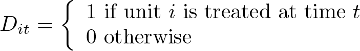
We focus on the estimation of treatment effects in the presence of binary time-varying treatment. Such a setting characterizes several economic and social policies and medical trials delivered over time. For example, one could be interested in assessing whether a certain treatment had an impact on a given target variable with some delay and whether anticipatory effects took place. To formalize this setting, let us start by considering a binary treatment indicator for individual i at time t:

$D_{it} =\{\begin{array}{l}\text{1} \text{if} \text{unit} i \text{is} \text{treated} \text{at} \text{time} t\\ 0\text{ otherwise}\end{array}$

Let us also assume an outcome equation with contemporaneous treatment plus one lag and one lead:

$Y_{it} ={\mu }_{it} +{\beta }_{-1}{D}_{it}{ }_{-1} +{\beta }_0{D}_{it} +{\beta }_{+1}{D}_{it}{ }_{+1} +\gamma x_{it} +u_{it}$

1

In (1), the β ₊₁ coefficient measures the impact of the treatment one period before its occurrence, and β ₋₁ measures the impact of treatment one period after it. x _it is a vector of covariates, γ is its conformable coefficient vector, and µ_it represents a fixed effect. Autor (2003) provided a first application of the treatment model implied by (1). ¹

For now, let us assume that treatment can occur only once over the interval [t−1, t+1] so that we can define the following sequences of possible treatments,

$\left\{w^j\right\}=\{D_{it}{ }_{-\text{1}}, D_{it}, D_{it}{ }_{+\text{1}}\}=\{\begin{array}{l}{w}^{\text{1}} = (0,0,0)\\ w^{\text{2}} = (\text{1},0,0)\\ w^{\text{3}} = (0,\text{1},0)\\ w^{\text{4}} = (0,0,\text{1})\end{array}$

2

where the sequence w ¹ is the usual benchmark of no treatment. The generic sequence is denoted as w^j (with j = 1,…, J and J = 4) and the associated potential outcome as $Y(w^j)$ . The “ATE between the two potential outcomes $Y(w^j)$ and $Y(w^k)$ ” can be easily defined as

${\text{ATE}}_{jk} =E \left\{Y_{it}\left(w^j\right) -Y_{it}\left(w^k\right)\right\}$

for j, k = 1,…, 4 and j ≠ k.

Under conditional mean independence—that is, conditioning on both x _it and the fixed effect µ_it —we have

$\begin{array}{c}\begin{array}{ccc}{\text{ATE}}_{jk} =E_{\text{x}}{ }_{,\mu } \left\{{\text{ATE}}_{jk} \left(x_{it}, {\mu }_{it}\right)\right\}& =& E_{\text{x}}{ }_{,\mu } \left[E Y_{it}\left(w^j,x_{it}, {\mu }_{it}\right)-Y_{it}\left(w^k,x_{it}, {\mu }_{it}\right)\right]\\ & =& E_{\text{x}}{ }_{,\mu } \left\{E \left(Y_{it}|w^j,x_{it}, {\mu }_{it}\right) -E\left(Y_{it}|w^k,x_{it}, {\mu }_{it}\right)\right\}\end{array}\\ \end{array}$

In such a model—with treatment occurring only once out of three periods, plus one lag and one lead of the treatment variable—we can define six possible ATEs that, for ease of reference, we collect in a matrix,

$\left[\begin{array}{ccccc} & w_{\text{1}}& w_{\text{2}}& w_{\text{3}}& w_{\text{4}}\\ w_{\text{1}}& -& & & \\ w_{\text{2}} & {\text{ATE}}_{\text{21}} & -& & \\ w_{\text{3}}& {\text{ATE}}_{\text{31}}& {\text{ATE}}_{\text{32}} & -& \\ w_{\text{4}}& {\text{ATE}}_{\text{41}}& {\text{ATE}}_{\text{42}}& {\text{ATE}}_{\text{43}} & -\end{array} \right]$

where the generic ATEjk represents the ATE of the sequence j against the counterfactual sequence k. Obviously, ATE _jk = −ATE _kj . Using (1) and the definition of w^j with j = 1,…, 4, we can show that

$\begin{array}{l}{\text{ATE}}_{\text{21}} =E(Y_{it}|w_{\text{2}})-E(Y_{it}|w_{\text{1}}) = (\overline{\mu }+{\beta }_{-}{ }_{\text{1}} +\gamma \overline{x})-(\overline{\mu }+\gamma \overline{x}) ={\beta }_{-}{ }_{\text{1}}\\ {\text{ATE}}_{\text{31}} =E(Y_{it}|w_{\text{3}})-E(Y_{it}|w_{\text{1}}) ={\beta }_0\\ {\text{ATE}}_{\text{41}} =E(Y_{it}|w_{\text{4}})-E(Y_{it}|w_{\text{1}}) ={\beta }_{+\text{1}}\\ {\text{ATE}}_{\text{32}} =E(Y_{it}|w_{\text{3}})-E(Y_{it}|w_{\text{2}}) ={\beta }_0 -{\beta }_{-\text{1}}\\ {\text{ATE}}_{\text{42}} =E(Y_{it}|w_{\text{4}})-E(Y_{it}|w_{\text{2}}) ={\beta }_{+\text{1}} -{\beta }_{-}{ }_{\text{1}}\\ {\text{ATE}}_{\text{43}} =E(Y_{it}|w_{\text{4}})-E(Y_{it}|w_{\text{3}}) ={\beta }_{+\text{1}} -{\beta }_0\end{array}$

In general, one obtains a number of ATEs equal to (J ²−J)/2, where J is the number of treatment sequences; in our example, we have (4² − 4)/2 = 6 ATEs. An important advantage of a dynamic treatment model is the ability to graphically plot the evolution of the treatment effects over time. To this end, let us define the predictions of Y_it given the sequence of treatments as

$E\left(Y_{it}|D_{it}{ }_{-\text{1}}, D_{it}, D_{it}{ }_{+\text{1}}, t\right)={\overline{\mu }}_t +{\beta }_{-\text{1}}{D}_{it}{ }_{-\text{1}} +{\beta }_0{D}_{it} +{\beta }_{+\text{1}}{D}_{it}{ }_{+\text{1}} +\gamma {\overline{x}}_t$

3

Consistently with the econometric practice, to make (3) computable, we assume additive separability; that is, µ_it = θ_i + δ_t , where θ_i and δ_t represent individual and time-fixed effects, respectively. It follows that ${\overline{\mu }}_{it} \equiv E({\mu }_{it}|D_{it}{ }_{-1}, D_{it}, D_{it}{ }_{+1}, t) =E({\mu }_{it}|t) =E({\theta }_i +{\delta }_t|t) =\overline{\theta }+{\delta }_t$ .

To keep things simple, let us restrict our attention only to the case of two specific treatment sequences,

$\begin{array}{l}{w}^T =\left\{. . . , D_{it}{ }_{-\text{2}} = 0, D_{it}{ }_{-\text{1}} = 0, D_{it} =\text{ 1}, D_{it}{ }_{+\text{1}} = 0, D_{it}{ }_{+\text{2}} = 0, . . .\right\}\\ w^C =\left\{. . . , D_{it}{{ }_{-}}_{\text{2}} = 0, D_{it}{{ }_{-}}_{\text{1}} = 0, D_{it} = 0, D_{it}{ }_{+\text{1}} = 0, D_{it}{ }_{+\text{2}} = 0, . . .\right\}\end{array}$

where w^T indicates the sequence in which treatment occurs only at time t and w^C indicates the no-treatment case. By setting A_it = {D_{it −1} , D_it, D_{it +1} , t} and iterating (3) one period back and one period forward, one obtains the prediction of Y at t − 1, t, and t + 1,

$\begin{array}{l}E(Y_{it}{ }_{-\text{1}}|A_{it}{ }_{-\text{1}}) ={\overline{\mu }}_t-\text{1} +{\beta }_{-\text{1}}{D}_{it}{ }_{-\text{2}} +{\beta }_0{D}_{it}{ }_{-\text{1}} +{\beta }_{+\text{1}}{D}_{it} +\gamma {\overline{x}}_t{ }_{-\text{1}}\\ E(Y_{it}|A_{it}) ={\overline{\mu }}_t+{\beta }_{-}{ }_{\text{1}}{D}_{it}{{ }_{-}}_{\text{1}} +{\beta }_0{D}_{it} +{\beta }_{+\text{1}}{D}_{it}{ }_{+\text{1}} +\gamma {\overline{x}}_t\\ E(Y_{it}{ }_{+\text{1}}|A_{it}{ }_{+\text{1}}) ={\overline{\mu }}_t+\text{1} +{\beta }_{-}{ }_{\text{1}}{D}_{it} +{\beta }_0{D}_{it}{ }_{+\text{1}} +{\beta }_{+\text{1}}{D}_{it}{ }_{+\text{2}} +\gamma {\overline{x}}_t{ }_{+\text{1}}\end{array}$

which can be used to calculate the expected outcome over t − 1, t, t + 1 conditional on w^T and w^C . Thus,

• for w^T , we have

$\begin{array}{c}E\left(Y_{it}{ }_{-\text{1}}|w^T =. . . ,0,0,\text{1},0,0, . . .\right) ={\overline{\mu }}_t-\text{1} +{\beta }_{+\text{1}} +\gamma {\overline{x}}_{t-1}\\ E\left(Y_{it}|w^T =. . . ,0,0,\text{1},0,0, . . .\right) ={\overline{\mu }}_t+{\beta }_0 +\gamma {\overline{x}}_t\\ E\left(Y_{it}{ }_{+\text{1}}|w^T =. . . ,0,0,\text{1},0,0, . . .\right) ={\overline{\mu }}_t+\text{1} +{\beta }_{-}{ }_{\text{1}} +\gamma {\overline{x}}_{t+1}\end{array}$

• for w^C , we have

$\begin{array}{c}E\left(Y_{it}{ }_{-\text{1}}|w^C =. . . ,0,0,0,0,0, . . .\right) ={\overline{\mu }}_t-\text{1} +\gamma {\overline{x}}_{ }{ }_{t-1}\\ E\left(Y_{it}|w^C =. . . ,0,0,0,0,0, . . .\right) ={\overline{\mu }}_t +\gamma {\overline{x}}_t\\ E\left(Y_{it}{ }_{+\text{1}}|w^C =. . . ,0,0,0,0,0, . . .\right) ={\overline{\mu }}_t+\text{1} +\gamma {\overline{x}}_t{ }_{t+1}\end{array}$

We can now plot these predictions over time (figure 1) and depict these situations:

Figure 1.

Pre- (t−1) and post- (t+1) treatment effect of a policy delivered at t. Source: Cerulli (2015, 202).

• If β ₊₁ ≠ 0, treatment delivered at time t affects the outcome at time t−1. Current treatment has an effect on past outcomes (anticipatory effect). Therefore, the pretreatment period is affected by current treatment.

• If β ₀ ≠ 0, treatment delivered at time t affects the outcome at time t, generating contemporaneous effects.

• If β ₋₁ ≠ 0, treatment delivered at time t affects the outcome at time t + 1. Current treatment has an effect on future outcomes (lagged effect). Therefore, the posttreatment period is affected by current treatment.

3 Testing the parallel-trend assumption

The pattern of the leads is also important to check for causality in the spirit of Granger (1969). Indeed, conditional on x _it and the fixed effect, if D_it causes Y_it , the leads should not be jointly different from zero in an equation like (1). A test for checking whether all the β _+s ’s are jointly equal to zero, s = 1,…, S, indirectly tests whether the parallel-trend assumption holds. Formally, we can define such a test as

$H_0:{\beta }_{+1}={\beta }_{+2}=\cdots ={\beta }_{+S}=0$

Note that rejecting H ₀ invalidates the causal interpretation of the estimates, while not rejecting H ₀ implies only a necessary condition for the parallel-trend to hold because the necessary and sufficient condition still remains untestable, being formulated on counterfactual unobservable quantities.

Another approach to test the parallel-trend assumption (still a necessary condition) requires dropping lags and leads from (1) and augmenting it with the time-trend variable t and its interaction with D_it . If the coefficient of the interaction term is statistically not significant, one can reasonably expect the parallel-trend assumption to hold (see Angrist and Pischke [2009, 238–239]).

To provide ground for such a test, let us write down the following potential-outcome model:

$\{\begin{array}{l}{Y}_{0,it}={\mu }_0+{\lambda }_{0}t+\gamma x_{it}+{\theta }_i+{\delta }_t+u_{0,it}\\ Y_{1,it}={\mu }_1+{\lambda }_{1}t+\gamma x_{it}\gamma +{\theta }_i+{\delta }_t+u_{1,it}\\ Y_{it}=Y_0{ }_{,it}+D_{it}\left(Y_{\text{1}}{ }_{,it}-Y_0{ }_{,it}\right)\end{array}$

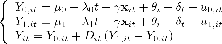
We allow again for an individual fixed effect (θ_i ) and a time effect (δ_t ), with the parameters λ ₁ and λ ₀ being the treated and untreated time trends, respectively. This way, by plugging the first two equations into the third one, we obtain

$Y_{it} ={\mu }_0 +{\lambda }_{0}t+\gamma x_{it} +D_{it}({\mu }_1 -{\mu }_0) +D_{it}t({\lambda }_1 -{\lambda }_0) +{\theta }_i +{\delta }_t +{\eta }_{it}$

with η_it = [u _0,it + D_it (u _1,it − u _0,it )]. Equivalently, we can write the previous equation as

$Y_{it} ={\mu }_0 +{\lambda }_{0}t+\gamma x_{it} +D_{it}\mu +D_{it} \times t\times \lambda +{\theta }_i +{\delta }_t +{\eta }_{it}$

which can be consistently estimated by a fixed-effects regression where the significance test for λ = (λ ₁ − λ ₀) provides a test for the parallel-trend assumption. Accepting the null H ₀: λ = 0 implies accepting that the parallel-trend assumption is not violated whenever one assumes no “anticipation effects”).

Finally, note that we can extend the previous test by also considering quadratic or even cubic time trends.

4 The tvdiff command

4.1 Description

tvdiff estimates ATEs in setups like the one just discussed, namely, when treatment is binary and varying over time. Using tvdiff, the user can estimate the pre- and postintervention effects by selecting the pre- and postintervention periods and plot the results in an easy-to-read graph. To assess the reliability of the causal interpretation of the results achieved by the user’s specified model, tvdiff allows one to test for the parallel-trend assumption using two tests, that is, the joint test on the leads and the time-trend test. tvdiff is a generalization of the DID approach to the case of many post- and preintervention times.

4.2 Syntax

The syntax of the command is as follows:

[tvdiff] outcome treatment varlist [if] [in] [weight ] , model( modeltype ) pre( # ) post( # ) test_tt graph save_graph( graphname ) vce( vcetype ) outcome is the target variable measuring the impact of treatment.

treatment is the binary treatment variable taking a value of 1 for treated units and a

value of 0 for untreated units.

varlist is the set of pretreatment (or observable confounding) variables.

aweights, fweights, and pweights are allowed; see [U] 11.1.6 weight.

4.3 Options

model( modeltype ) specifies the estimation model, where modeltype must be fe (fixed effects) or ols (OLS). model() is required.

pre( # ) specifies the number (#) of pretreatment periods. pre() is required.

post( # ) specifies the number (#) of posttreatment periods. post() is required.

test_tt performs the parallel-trend test using the time-trend approach. The default is to use the leads.

graph allows for a graph of the results. It uses the coefplot command implemented by Jann (2014).

save_graph( graphname ) allows one to save the graph as graphname.

vce( vcetype ) allows for robust and clustered regression standard errors in the model’s estimates.

4.4 Remarks

tvdiff creates the following variables:

• _D_L1,…, _D_L m are the lags of the treatment variable, with m equal to # in the post( # ) option.

• _D_F1,…, _D_F p are the leads of the treatment variable, with p equal to # in the pre( # ) option.

Finally, note that i) the treatment has to be a 0/1 binary variable (1 = treated, 0 = untreated) and that ii) before running tvdiff, one has to install the community-contributed command coefplot (Jann 2014).

4.5 Stored results

tvdiff stores the following in e():

5 An application using simulated data in the presence of selection bias

This example shows how to correctly run tvdiff and shows how it solves the selection bias that often arises in real causal inference applications.

For this purpose, we design a simulated DGP allowing for a nonzero correlation between the “selection equation” or “treatment equation” (the D-equation) and the “outcome equation” (the y-equation), due to the presence of unobservable selection as captured by an individual specific effect acting as confounder.

Consider the same treatment setting of (1); that is, only one lead and one lag are included. Exclude, without loss of generality, observable confounders x. Below, we show that (1) can be derived from a generalized potential-outcome model made of three treatments, that is, the treatment sequences set out in (2):

$y_{it} =y_{it}(w\text{1}) +D_{it}{{ }_{-}}_{\text{1}} \left\{y_{it} \left(w^2\right) -y_{it} \left(w^1\right) \right\}+D_{it} \left\{y_{it} \left(w^3 \right)-y_{it} \left(w^1\right) \right\}+D_{it}{ }_{+\text{1}} \left\{y_{it} \left(w^4 \right)-y_{it} \left(w^1\right)\right\}$

4

Assume that the potential outcome takes on this form

$y_{it}\left(w^j\right) = {\beta }_j + u_{it}^j = {\beta }_j + {\epsilon }_{it}^j + c_i$

5

where $u_{it}^j=c_i+{\epsilon }_{it}^j$ . c_i represents the individual fixed effect, ${\epsilon }_{it}^j$ represents a pure random shock, and β_j is a parameter to be estimated. By substituting (5) into (4), we can see that

$y_{it} = ({\beta }_1 +c_i) +D_{it}{ }_{-1}({\beta }_2 -{\beta }_1) +D_{it}({\beta }_3 -{\beta }_1) +D_{it}{ }_{+1}({\beta }_4 -{\beta }_1) +{\eta }_{it}$

6

where ${\eta }_{it}={\epsilon }_{it}^1+D_{it-1}\left({\epsilon }_{it}^2-{\epsilon }_{it}^1\right)+D_{it}\left({\epsilon }_{it}^3-{\epsilon }_{it}^1\right)+D_{it+1}\left({\epsilon }_{it}^4-{\epsilon }_{it}^1\right).$

Equation (6) is equivalent to (1), apart from x _it , under the specification β ₋₁ = β ₂ − β ₁, β ₀ = β ₃ − β ₁, β ₊₁ = β ₄ − β ₁, µ_it = β ₁ + c_i , and finally, u_it = η_it .

By using the definitions of ATE _jk , we can finally rewrite (6) as

$y_{it} ={\beta }_1 +c_i +D_{it}{ }_{-1}AT{E}_{21} +D_{it}AT{E}_{31} +D_{it}{ }_{+1}AT{E}_{41} +{\eta }_{it}$

We can now perform our simulation experiment showing that tvdiff with the option model(fe), unlike the option model(ols), can solve a selection-on-unobservables problem. The DGP is such that the individual effect c_i feeds into both the potential outcomes, through the error term, and the selection equation for D_it :

$\begin{array}{l}{c}_i \sim \text{normal}\left(3,1\right)\\ u_{it}^j =c_i^3 +{\epsilon }_{it}^j.\\ j= 1,2,3,4\\ {\epsilon }_{it} \sim \text{normal}\left(0,1\right)\\ D_{it} =1(10 \times c_i +{\epsilon }_{it} >0)\\ {\beta }_1 = 10, {\beta }_2 = 20, {\beta }_3 = 30, {\beta }_4 = 40\end{array}$

Observe that c_i enters the potential outcomes’ random shocks, $u_{it}^j$ , nonlinearly. This choice depends on the fact that D_it is modeled as binary and nonlinear within this DGP, thus requiring a nonlinear form of the fixed effect in the potential-outcome equations to produce substantial OLS bias. Below is the code for this DGP:

We run tvdiff twice, once with the option model(ols) and once with model(fe):

As expected, because of the correlation between the outcome equation and the selection equation entailed by this DGP, OLS estimates are severely biased. The OLS coefficient of the lead—expected to be equal to 30—is in fact equal to about 65, and large biases also arise for the contemporaneous and the lagged coefficients (respectively, about 56 instead of 20 and about 44 instead of 10). On the contrary, the fixed-effects estimator performs well, with all the coefficients close to the true coefficients, thus showing that it effectively solves the selection bias underlying this DGP. Introducing exogenous variables within the previous DGP does not change these results.

6 An application to the effect of public education expenditure on income equality

In this section, we provide an application of tvdiff to real data. We apply tvdiff to measure the effect of public education effort on income equality at the country level. To this end, we use the longitudinal data of Castellacci and Natera (2011) to build cana.dta. This dataset is a rich and complete set of 41 indicators for 134 countries observed over the 1980–2008 period for a total of 3,886 country-year observations. Castellacci and Natera’s (2011) data are publicly available and allow for detailed cross-country analyses of national systems, growth, and development.

Within these data, public education effort is measured as the (current and capital) total public expenditure on education as a percentage of gross domestic product (GDP) (variable es12educe), while income equality is measured as the complement of the Gini index (variable sc8ginii). In this application, we consider as controls the following covariates as found in Castellacci and Natera (2011):

• i3teler: Telecommunication Revenue. Revenue from the provision of telecommunications services such as fixed-line, mobile, and data, % of GDP.

• i4elecc: Electric power consumption. Production of power plants and combined heat and power plants less transmission, distribution, and transformation losses and own use by heat and power plants.

• i6telecap: Mobile and fixed-line subscribers. Total telephone subscribers (fixed line plus mobile) per 1000 inhabitants.

• ec16openi: Openness Indicator. (Import + Export)/GDP. PPP, 2000 USD.

• sc20trust: Most people can be trusted. Percentage of respondents who “agree” with this statement.

• ec14credg: Domestic Credit by Banking Sector. Includes all credit to various sectors on a gross basis, with the exception of credit to the central government, which is net, as a share of GDP.

• pf20demoa: Index Democracy and Autocracy. Democracy: political participation is full and competitive, executive recruitment is elective, constraints on the chief executive are substantial. Autocracy: it restricts or suppresses political participation. The index ranges from +10 (democratic) to −10 (autocratic).

The binary treatment D_it is defined as follows: consider the “within” median of public expenditure in education over GDP, namely, the median by country of the share of public expenditure in education over GDP for the 1980–2008 period. If in year t, country i performs a public expenditure in education larger than its “within” median, then D_it = 1 (the pair country-year is thus “treated”); otherwise, D_it = 0. In other words, the treatment is defined as the tendency of a country to boost its expenditure in education in a specific year compared with a baseline reference, measured as its median performance over the overall time span. The outcome y is measured as the “total public expenditure in education as a percentage of GDP”.

We do this exercise by running the following code, where tvdiff is used with five pretreatment periods and nine posttreatment periods:

For brevity’s sake, the regression outputs are omitted, ensuring that both parallel-trend tests are passed, and we focus on the graph in figure 2. This figure shows that from the time of treatment (that is, higher than the median education expenditure) onward, the ATE, given by the level of equality in income distribution, increases steeply and remains positive until the seventh year after treatment.

Figure 2.

Graph of the pre- and posttreatment pattern for the relation between country investment in public education and income equality

The pattern is a sort of parabola, showing that the effect of one short increase in education expenditure above the median has a transitory effect tending to fade away around seven years after treatment. Considering that significance is relatively high after 3, 4, and 5 years from treatment time (t), this finding shows a quite sensible effect of public investment in education on income equality. More specifically, we see that the (average) equality index difference between treated and untreated reaches a value of around 0.5% three and four years after treatment and then decreases in the subsequent years.

Of course, other possible confounders may be present. However, the use of fixed-effects estimation should mitigate unobservable selection, thus making these results also sufficiently robust to selection on unobservables. This is one of the main strengths of DID that tvdiff helps to apply.

7 Conclusion

In this article, we presented tvdiff, a community-contributed command for estimating ATEs when the treatment is binary and varying over time. We introduced the econometrics underlying the model fit by tvdiff and showed the possibility to graph the estimated effects. Subsequently, we showed the logic of the two parallel trends tests and how to carry them out with tvdiff. We finally presented the command’s syntax and provided two applications: one on simulated data and one on real data evaluating the effect of public education expenditure on income equality.

Note that one must be cautious when using this command for causal inference because both tests allow for testing only the necessary condition for identification to hold. Hence, if the parallel trend is supported by the tests, the user should validly motivate why the sufficient condition is expected to hold under the specific context of analysis.

We hope readers will find tvdiff useful for practical program evaluation in appropriate contexts. We envision further developments to extend this command to multivalued and continuous treatment settings.

9 Programs and supplemental materials

Supplemental Material, st0566 - Estimation of pre- and posttreatment average treatment effects with binary time-varying treatment using Stata

Supplemental Material, st0566 for Estimation of pre- and posttreatment average treatment effects with binary time-varying treatment using Stata by Giovanni Cerulli and Marco Ventura in The Stata Journal