Sage Journals: Discover world-class research

Abstract

In this article, we present new commands for modeling count data using marginalized zero-inflated distributions. While we mainly focus on presenting new commands for estimating count data, we also present examples that illustrate some of these new commands.

Keywords

st0563 mzip mzip postestimation mzigp mzigp postestimation mzinb mzinb postestimation marginalized count data Poisson generalized Poisson negative binomial zero-in flated

1 Introduction

Often, count responses have zero-inflation—a higher prevalence of zeros than is accounted for by the underlying distribution of the regression model to be fit. This discordance can occur for outcome variables in many fields of study, such as medical, public health, and manufacturing. In these cases, estimation based on the distributional assumptions of Poisson, generalized Poisson, and negative binomial models can result in incorrect parameter estimates and biased standard errors. Zero-inflated count data are encountered in the number of defects in manufacturing (Lambert 1992), patient falls in hospitals (Ullah, Finch, and Day 2010), and the number of cubes in the test of tower building for motor development (Cheung 2002), just to name a few. Hardin and Hilbe (2018) describe the two origins of zero outcomes: outcomes for individuals who do not enter into the counting process and outcomes for individuals who enter into the counting process and have a zero outcome. Mullahy (1986) proposed the zero-inflated Poisson (ZIP) model, using a model familiar to researchers (Poisson), to deal with outcomes with an excess of zeros. However, for modeling count data with zero outcomes where overdispersion or underdispersion exists, one should consider other models, such as zero-inflated generalized Poisson (ZIGP) and zero-inflated negative binomial (ZINB) (Famoye and Singh 2006; Greene 1994).

Sometimes analysts want to estimate the marginal mean and be able to interpret estimated coefficients as the population-average parameters. Some authors have proposed different approaches to marginal models, such as Lee et al. (2011), who proposed likelihood-based marginalized models for zero-inflated clustered count data using hurdle models. Kassahun et al. (2014) presented ways to model hierarchical count data that had issues such as overdispersion, correlation, and an excess of zeros by marginalized hurdle and marginalized ZIP (MZIP) normal-gamma models. Others, like Heagerty and Zeger (2000), used a marginalized multilevel model that regressed the marginal mean instead of the conditional mean on the covariates. Long et al. (2014) recently proposed an MZIP regression model that directly models the population mean count, therefore providing the ability to interpret population-wide parameters. Preisser et al. (2016) also proposed a marginalized zero-inflated negative binomial (MZINB) regression model and applied it on dental caries in a school-based fluoride mouth rinse program.

We introduce the new commands mzip, for the marginalized zero-inflated Poisson (MZIP) regression model presented in Long et al. (2014), and mzinb, for the MZINB regression model presented in Preisser et al. (2016). We also extend that method to include a marginalized zero-inflated generalized Poisson (MZIGP) regression model and its accompanying command.

In this article, we illustrate modeling count data using MZIP, MZIGP, and MZINB regression models. In section 2, we review the three marginalized zero-inflated regression models. In section 3, we present syntax for the new commands. In section 3, we present a synthetic data example and a real world data example. Finally, we summarize in section 5.

2 Marginalized zero-inflated distributions

2.1 Marginalized ZIP distribution

The widely known ZIP regression model with a count outcome variable, Y_i (i = 1,…, n), has the probability p_i that the binary process results in a zero outcome, where 0 ≤ p_i < 1, and the counting process probability of a zero outcome is from the Poisson distribution. Thus, we have a probability mass function (p.m.f.)

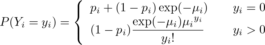
P (Y_{i} = y_{i}) = {\begin{cases} p_{i} + (1 - p_{i}) exp ({- µ}_{i}) y_{i} = 0 \\ (1 - p_{i}) \frac{exp (- µ_{i}) {µ_{i}}^{y_{i}}}{y_{i}!} y_{i} > 0 \end{cases}

where µ_i = exp(x_iβ) and p_i = g⁻¹(z_iγ) and where g⁻¹(·) is the inverse link function of the linear predictor z_iγ; our software allows specification of inverse link functions for logit, probit, loglog, and complementary loglog.

For a random sample of observations y₁, y₂,…, y_n, the MZIP regression log-likelihood function is given by

L = \sum_{i \in Z} [\ln {p_{i} + (1 - p_{i}) \exp (- μ_{i})}] + \sum_{i \notin Z} {\ln (1 - p_{i}) - μ_{i} + y_{i} \ln (μ_{i}) - Γ (y_{i} + 1)}

where the mean (µ_i) is rescaled from the ZIP regression model to µ_i = exp{x_iβ − ln(1 − p_i)} and Z is the set of zero outcomes.

2.2 MZIGP distribution

The ZIGP regression model with a count outcome variable, Y_i, where i = 1,…, n, has the p.m.f.

\begin{array}{l} p (Y_{i} = y_{i}) = {\begin{cases} p_{i} + (1 - p_{i}) \exp (- μ_{i}) y_{i} = 0 \\ (1 - p_{i}) \frac{μ_{i} (μ_{i} + δ y_{i})^{y_{i} - 1} \exp (- μ_{i} - δ y_{i})}{y_{i}!} y_{i} > 0 \end{cases} \end{array}

where µ_i = exp(x_iβ), p_i = g⁻¹(z_iγ), and δ is the dispersion parameter having 0 ≤ δ < 1. By applying the same concept from the MZIP regression model in section 2.1 to the ZIGP regression model, we introduce the MZIGP regression model. For a random sample of observations y₁, y₂,…, y_n, the MZIGP regression log-likelihood function is

L = \sum_{i \in Z} [ln {p_{i} + (1 - p_{i}) exp (- μ_{i})}] + \sum_{i \notin Z} {ln (1 - p_{i}) + In (μ_{i}) + (y_{i} - 1) In (μ_{i} + δ y_{i}) - μ_{i} - δ y_{i} - In Γ (y_{i} + 1)}

where the mean (µ_i ) is rescaled from the ZIGP regression model to µ_i = exp{x_iβ−ln(1− p_i )}, δ is the dispersion parameter having 0 ≤ δ < 1, and Z is the set of zero outcomes.

2.3 MZINB distribution

The ZINB regression model with a count outcome variable Y_i , where i = 1,…, n, has the p.m.f.

\begin{array}{l} p (Y_{i} = y_{i}) = {\begin{cases} p_{i} + (1 - p_{i}) {(\frac{1}{1 + δ μ_{i}})}^{(\frac{1}{δ})} y_{i} = 0 \\ (1 - p_{i}) \frac{Γ (\frac{1}{δ + y_{i}})}{Γ (y_{i} + 1) Γ (\frac{1}{δ})} {(\frac{1}{1 + δ μ_{i}})}^{\frac{1}{δ}} {(1 - \frac{1}{1 + δ μ_{i}})}^{y_{i}} y_{i} > 0 \end{cases} \end{array}

where µ_i = exp(x_iβ), p_i = g ⁻¹(z_iγ), and δ is the dispersion parameter. Lastly, we apply the same concept from the MZIP regression model in section 2.1 to the ZINB regression model, and we introduce the MZINB regression model. For a random sample of observations y ₁ , y ₂ ,…, y_n , the MZINB regression log-likelihood function is

L = \sum_{i \in Z} \ln {p_{i} + (1 - p_{i}) {(\frac{1}{1 + δ μ_{i}})}^{\frac{1}{δ}}} + \sum_{i \notin Z} [\ln (1 - p_{i}) + \ln Γ {(\frac{1}{δ}) + y_{i}} - \ln Γ (y_{i} + 1) - \ln Γ (\frac{1}{δ}) + (\frac{1}{δ}) \ln (\frac{1}{1 + δ μ_{i}}) + y_{i} \ln (1 - \frac{1}{1 + δ μ_{i}})]

where the mean (µ_i ) is rescaled from the ZINB regression model to µ_i = exp{x_iβ−ln(1− p_i )}, δ is the dispersion parameter, and Z is the set of zero outcomes.

3 Syntax

The accompanying software includes the command files and supporting files for prediction and help. In the following syntax diagrams, unspecified options include the usual collection of maximization and display options available for all estimation commands. All marginalized zero-inflated commands include the ilink( linkname )option to specify the link function for the inflation model. Allowable arguments to the ilink() option include logit, probit, loglog, or cloglog.

Equivalent in syntax to the zip command, the basic syntax for specifying an MZIP model for count data is

mzip depvar indepvars if in [ weight ] , inflate( varlist [ , offset( varname ) ]| cons) [ options ] The syntax for specifying an MZIGP distribution for count data is

mzigp depvar indepvars if in weight , inflate( varlist [ , offset( varname ) ]| cons) [ options ] The syntax for specifying an MZINB distribution for count data is

mzinb depvar [ indepvars ] if in weight , inflate( varlist [ , offset( varname ) ] | cons) [ options ]

4 Examples

4.1 Example synthetic marginalized zero-inflated data

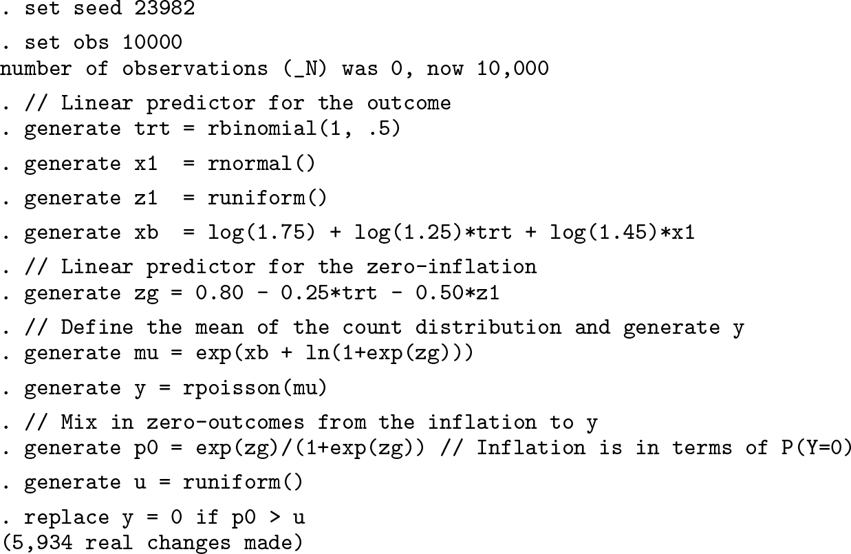
Here we illustrate how to generate synthetic marginalized zero-inflated data. We synthesized trt from a Bernoulli(0.5) and x ₁ from a normal(0, 1). The true parameter values are {γ ₀ = 0.80, β ₀ = log(1.75), γ ₁ = −0.25, β ₁ = log(1.25), γ ₂ = −0.50, β ₂ = log(1.45)} (see parameter definitions and references in section 2.1). To highlight the differences between using nonzero-inflated and nonmarginalized zero-inflated models compared with marginalized zero-inflated models, we will fit our data with three separate models— Poisson, ZIP, and MZIP. We will also highlight the use of the average predicted value described in Albert, Wang, and Nelson (2014) to estimate the total effect of the trt variable in the ZIP model.

Having created an outcome with our specified associations, we can fit some models (below) to see how closely the sample data match the specifications. The first model using our marginalized zero-inflated synthesized data with a Poisson distribution shows that using the robust variance estimator does a good job adjusting for the overdispersion due to the excess zeros (compared with the marginalized ZIP results at the end of this section).

However, when we fit our ZIP model to our sample data, we see a worse match to our synthetic-data specifications. The estimated coefficients for both of the nonzero-inflated components are not close to the values from our synthesized data. However, we can use a program to calculate the difference and ratio versions of the average predicted value.

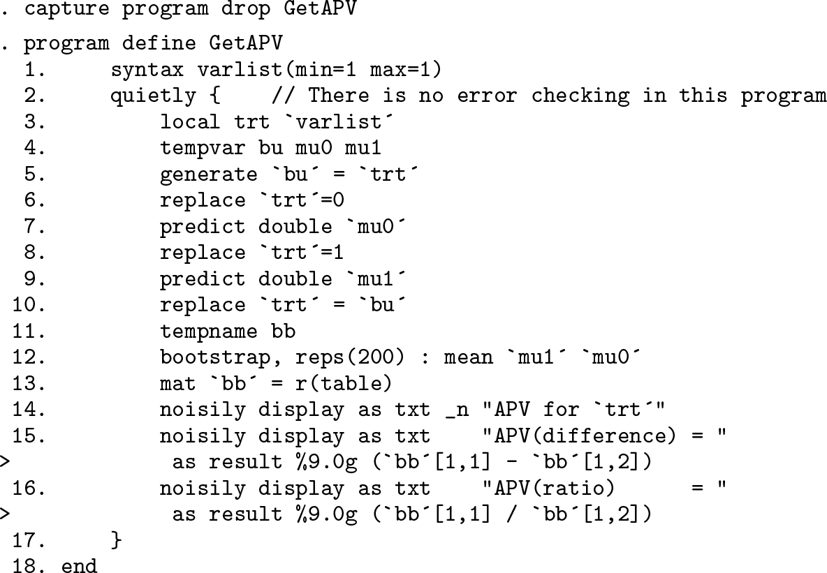
The ratio version of the average predicted value depicted above illustrates the total estimated effect of the trt variable. This same effect is what is estimated by the Poisson and MZIP models. That is, when the value of trt is changed, it affects the rate and probability of zero-outcomes.

Finally, we fit the data with the MZIP regression model with requested exponentiated coefficients. As expected, because the data are generated according to this model, they are well estimated.

4.2 Example real-world study

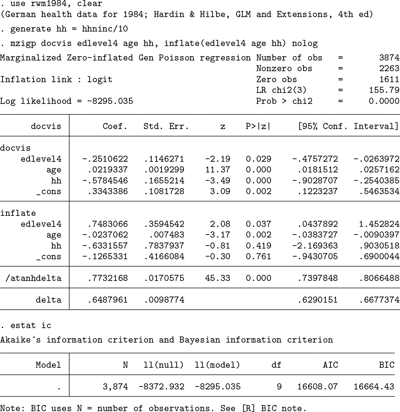
We use the popular German health reform data for the year 1984 as example data. The goal of our example is to understand the number of visits made to a physician during 1984. Our predictor of interest is whether the patient is highly educated based on achieving a graduate degree (edlevel4), for example, MA/MS, MBA, PhD, or a professional degree. Confounding predictors are age (age) ranging from 25–64 and income in German marks (hhninc) divided by 10. Almost half the time (42%), the patients did not visit the doctor (excess zero counts). Therefore, a zero-inflated model would be appropriate to model this data. We model the data using our MZIGP and MZINB regression models, which we explained earlier.

From the output, variables edlevel4 and age appear to affect zero counts, with younger graduate patients less likely to see a physician at all during the year. Patients not at the graduate level made about 22% [exp(−0.251)] fewer visits than graduate school patients. All three variables (edlevel4, age, hh) affect the nonzero counts significantly at α = 0.05. Also note that the dispersion parameter δ = 0.6488 is statistically significant, showing the overdispersion in the data.

Similarly, from the output, variables edlevel4 and age appear to affect zero counts, with younger graduate patients less likely to see a physician at all during the year. Patients not at the graduate level made about 26% [exp(−0.298)] fewer visits than graduate school patients. All three variables (edlevel4, age, hh) affect the nonzero counts significantly at α = 0.05. Also note that the dispersion parameter δ = 1.865 is statistically significant, showing the overdispersion in the data. The Akaike information criterion and Bayesian information criterion statistics are slightly lower in the MZIGP regression model, indicating a much better fit than the MZINB regression model.

5 Summary

In this article, we introduced supporting programs for modeling count data using marginalized zero-inflated distributions. We illustrated the use of the new command mzip using synthesized data, and we illustrated the new commands mzigp and mzinb using real-world German health data from 1984.

6 Programs and supplemental materials

To install a snapshot of the corresponding software files as they existed at the time of publication of this article, type

Supplemental Material

Supplemental Material, st0563 - Modeling count data with marginalized zero-inflated distributions

Supplemental Material, st0563 for Modeling count data with marginalized zero-inflated distributions by Tammy H. Cummings and James W. Hardin in The Stata Journal

References

Albert

J. M.

Wang

Nelson

. 2014. Estimating overall exposure effects for zero-inflated regression models with application to dental caries. Statistical Methods in Medical Research 23: 257–278.

Cheung

Y. B.

2002. Zero-inflated models for regression analysis of count data: A study of growth and development. Statistics in Medicine 21: 1461–1469.

Famoye

Singh

. 2006. Zero-inflated generalized Poisson regression model with an application to domestic violence data. Journal of Data Science 4: 117–130.

Greene

W. H.

1994. Accounting for excess zeros and sample selection in Poisson and negative binomial regression models. Working Paper Series EC-94-10, Department of Economics, Stern School of Business, New York University.

Hardin

J. W.

Hilbe

J. M.

. 2018. Generalized Linear Models and Extensions. 4th ed. College Station, TX: Stata Press.

Heagerty

P. J.

Zeger

S. L.

. 2000. Marginalized multilevel models and likelihood inference. Statistical Science 15: 1–19.

Kassahun

Neyens

Molenberghs

Faes

Verbeke

. 2014. Marginalized multilevel hurdle and zero-inflated models for overdispersed and correlated count data with excess zeros. Statistics in Medicine 33: 4402–4419.

Lambert

1992. Zero-inflated Poisson regression, with an application to defects in manufacturing. Technometrics 34: 1–14.

Lee

Joo

Song

J. J.

Harper

D. W.

. 2011. Analysis of zero-inflated clustered count data: A marginalized model approach. Computational Statistics & Data Analysis 55: 824–837.

10.

Long

D. L.

Preisser

J. S.

Herring

A. H.

Golin

C. E.

. 2014. A marginalized zeroinflated Poisson regression model with overall exposure effects. Statistics in Medicine 33: 5151–5165.

11.

Mullahy

1986. Specification and testing of some modified count data models. Journal of Econometrics 33: 341–365.

12.

Preisser

J. S.

Das

Long

D. L.

Divaris

. 2016. Marginalized zero-inflated negative binomial regression with application to dental caries. Statistics in Medicine 35: 1722–1735.

13.

Ullah

S.C.

Finch

Day

. 2010. Statistical modelling for falls count data. Accident Analysis and Prevention 42: 384–392.

Supplementary Material

Please find the following supplemental material available below.

For Open Access articles published under a Creative Commons License, all supplemental material carries the same license as the article it is associated with.

For non-Open Access articles published, all supplemental material carries a non-exclusive license, and permission requests for re-use of supplemental material or any part of supplemental material shall be sent directly to the copyright owner as specified in the copyright notice associated with the article.

0.02 MB

0.00 MB