Sage Journals: Discover world-class research

Abstract

Researchers who model fractional dependent variables often need to consider whether their data were generated by a two-part process. Two-part models are ideal for modeling two-part processes because they allow us to model the participation and magnitude decisions separately. While community-contributed commands currently facilitate estimation of two-part models, no specialized command exists for fitting two-part models with process dependency. In this article, I describe generalized two-part fractional regression, which allows for dependency between models’ parts. I show how this model can be fit using the community-contributed cmp command (Roodman, 2011, Stata Journal 11: 159–206). I use a data example on the financial leverage of firms to illustrate how cmp can be used to fit generalized two-part fractional regression. Furthermore, I show how to obtain predicted values of the fractional dependent variable and marginal effects that are useful for model interpretation. Finally, I show how to compute model fit statistics and perform the RESET test, which are useful for model evaluation.

Keywords

st0558 generalized two-part fractional regression process dependence fractional probit cmp

1 Introduction

In many disciplines, researchers need to fit regression models where the dependent variable is in the form of a fraction, percentage, or proportion. In finance, a commonly examined fractional dependent variable (FDV) is the financial leverage ratio of firms, that is, the amount of debt a firm issues relative to its amount of capital. Empirical research suggests that the financial leverage decision of firms is best described as a two-step process; first, the firm decides whether to issue debt, and then it decides how much debt to issue (Ramalho and da Silva 2009). However, the process determining which firms choose to issue debt is nonrandom because firms self-select into a leveraged position. Thus, we need a model that not only can separate the effects on the debt versus no debt from the effects on the amount-of-debt decision but also can account for the nonrandom selection that leads to some firms issuing debt. The generalized two-part fractional regression model (GTP-FRM) is such a model.

Before we dig into the GTP-FRM, I will give a short introduction on modeling FDVs. Modeling an FDV requires a fractional regression model (FRM). If we use the quasi– maximum likelihood estimator (QMLE) and the logit link, the model is known as the fractional logit; it is known as the fractional probit if we use the probit (Papke and Wooldridge 1996). An FRM is preferable because it ensures predictions within the unit interval and requires only correct specification of the conditional mean. Estimation of FRMs with various link functions is straightforward in Stata with the glm command and has become even more accessible with the Stata 14 addition of the fracreg command.

In many cases, an FDV may contain many values at one or both boundaries. The values at, for example, the zero boundary may be governed by a different process than the values between the boundaries. For instance, the covariates that affect a firm’s decision to issue debt are likely to be different from those affecting how much debt to issue (Cook, Kieschnick, and McCullough 2008). For such purposes, Ramalho and da Silva (2009) proposed a two-part fractional model (TP-FRM). The TP-FRM allows for specification of a binary model for the participation decision (y = 0 versus y > 0), for example, debt versus no debt, and an FRM for the magnitude decision (the magnitude of y when y > 0), such as how much debt to issue. Using this model, we allow the effects of a covariate on the participation decision to be different from the magnitude decision. In Stata, TP-FRMs can be fit using the community-contributed frm (Ramalho, Ramalho, and Murteira 2011) or tpm (Belotti et al. 2015) command.

In some cases, we may need even more flexibility than what is offered by the TP-FRM, such as when the participation and magnitude decisions are dependent. Continuing the example from above, there may be a selection bias in the types of firms that choose to issue debt. This problem is analogous to the well-known sample selection problem. Recently, Schwiebert and Wagner (2015) proposed the GTP-FRM as a means to model fractional two-part processes with dependence. The GTP-FRM formulation is advantageous because it nests the TP-FRM as a special case when the two processes are independent.

Currently, the GTP-FRM does not have a dedicated Stata command. In this article, I demonstrate how Stata users can fit GTP-FRMs by using the conditional mixed-process framework implemented by the cmp (Roodman 2011) command. In section 2, I briefly describe the GTP-FRM. In section 3, I give a short tutorial showing how to use cmp to fit the GTP-FRM, and I demonstrate how to compute predictions, marginal effects, information criteria, and RESET test statistics. In section 4, I provide a short conclusion.

2 Brief review of generalized two-part fractional regression

In many practical applications, FDVs naturally give rise to many zeros. For example, some firms do not have any exports (0% of total sales attributed to foreign sales), some individuals do not smoke (0% of their income spent on cigarettes), and some firms do not issue any debt (0% leveraged capital). When encountering such FDVs, researchers must decide how to qualitatively interpret the zeros (Ramalho, Ramalho, and Murteira 2011), because the zeros may actually be best described by a different mechanism than the positive values. Consider, for instance, the financial leverage decisions of firms. While a financing life-cycle approach would argue that older firms are more likely to issue debt, pecking-order theory would suggest that older firms prefer a lower proportion of debt because of a large amount of accumulated retained earnings (Ramalho and da Silva 2009). In such cases, a TP-FRM is ideal because it allows us to model the participation and magnitude decisions separately.

If a two-part process constitutes the best description of our data, we need to consider whether the two decisions are dependent. If unobserved factors affecting the decision to issue debt are correlated with factors that influence the proportion of debt sought by firms, the TP-FRM estimates will be biased (Wooldridge 2010). For instance, research suggests that a moderate degree of CEO narcissism is associated with greater corporate risk taking (Aabo and Eriksen 2018). If CEO narcissism is related to firm profitability but is not accounted for, then the estimate of firm profitability on the proportion of debt is likely to be biased. The GTP-FRM models the correlation between the two decisions, thus attempting to both estimate and adjust for the dependency between the processes. This makes the GTP-FRM ideal for FDVs best described by dependent two-part processes.

2.1 Model formulation

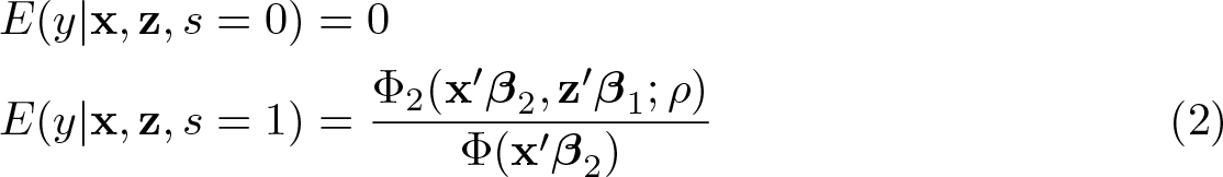
Following Schwiebert and Wagner (2015), we start by specifying the process determining the participation decision, where we assume an FDV, y, with values in the unit interval:

s = 1 (z^{'} β_{1} + u > 0)

where s is an indicator variable that takes the value 1 if the value of the outcome, y, is nonzero; z is a vector of covariates affecting the participation decision; β ₁ is a vector of coefficients; and u is the error term. To model the participation decision in (1), we use a probit model specification,

Pr (s = 1 | z) = Φ (z^{'} β_{1})

where Φ(·) is the standard normal cumulative distribution function. We specify the conditional mean of the magnitude decision as follows:

\begin{array}{l} E (y | x, z, s = 0) = 0 \\ E (y | x, z, s = 1) = \frac{Φ (x^{'} β_{2}, z^{'} β_{1}; ρ)}{Φ (x' β_{2})} \end{array}

x is a vector of covariates affecting the magnitude decision, β ₂ is a coefficient vector with respect to x, and Φ₂(·) denotes the bivariate standard normal distribution with ρ representing the correlation between the participation and magnitude decisions. Equation (2) is the fractional probit specification, which is used to model nonzero values of y. If the two processes in (2) are independent—that is, if ρ = 0—then the GTP-FRM reduces to the simpler TP-FRM, where E(y|x, z , s = 1) = Φ(x ^′ β ₂). However, if ρ > 0, then the TP-FRM is misspecified. The larger the dependence between the two processes, the larger the bias we would expect by using a TP-FRM.

Based on the above formulation, the GTP-FRM is clearly a more complicated model than the TP-FRM. In contrast to the TP-FRM, the GTP-FRM lets both x and z affect the magnitude decision: While x has a direct effect, the effect of z is indirect through s (Schwiebert and Wagner 2015). This extra complexity does not come for free. Indeed, the GTP-FRM needs an exclusion restriction to be identified; that is, it needs a variable affecting the participation decision without directly affecting the amount decision. Though we may be able to fit a GTP-FRM without an exclusion restriction in practice, we should not trust its estimates (Sartori 2003).

2.2 Marginal effects

As for the regular binary probit model, we should abstain from interpreting the model coefficients directly. Instead, we should rely on marginal effects preferably accompanied by graphical illustrations of predicted values of the FDV (Wulff 2015). As shown by Schwiebert and Wagner (2015), the predicted values of the FRM given values of the covariates are given by

E (y | x, z) = E (y | x, z, s = 1) Pr (s = 1 | z)

= Φ_{2} (x^{'} β_{2}, z^{'} β_{1}; ρ)

As for other two-part models, it is possible to obtain other types of predictions based on the GTP-FRM. For instance, we can compute the expected value of y conditional on y > 0, that is, the term E(y|x, z , s = 1).

Based on (4), the marginal effect of x_k in the GTP-FRM is given by

\frac{\partial E (y | x, z)}{\partial x_{k}} = \frac{\partial Φ_{2} (x^{'} β_{2}, z^{'} β_{1}; ρ)}{\partial x_{k}}

As I illustrate later, marginal effects and predicted values of the FDV can be obtained using margins after fitting the model using cmp. We will especially need to use (3) to obtain the predicted values of the FRM and the corresponding marginal effects.

2.3 Model fit measures

When comparing various fractional model specifications, we can rely on the Akaike information criterion (AIC) and Bayesian information criterion (BIC). Comparing measures based on pseudolikelihoods from different models can be tricky. Papke and Wooldridge (1996) argue for defining R ² in terms of the actual and predicted values. Like R ², information criteria can also be defined in terms of the residual sum of squares (RSS). Thus, I suggest using the following definitions of AIC and BIC when comparing FRMs, TP-FRMs, and GTP-FRMs:

AIC = log (\frac{RSS}{n}) + \frac{2 K}{n}

BIC = log (\frac{R S S}{n}) + \frac{K log (n)}{n}

where n is the sample size and K is the total number of parameters from each part of the GTP-FRM. Defining information criteria in this way has two major advantages when working with FDVs. First, they are comparable across any model for the conditional mean and for any estimation method (Papke and Wooldridge 1996). For instance, we can compare our GTP-FRM with its tobit equivalent—the exponential type II tobit model for corner solution responses (Wulff and Villadsen 2018). Second, we do not have to worry about unintentionally comparing information criteria across models with different (pseudo)likelihood functions.

2.4 RESET test

For the GTP-FRM, we can use Ramsey’s (1969) RESET test as a simple functional form diagnostic. Essentially, the test can be used to check for missing nonlinearities in the GTP-FRM or any other index model (Pagan and Vella 1989). For each model part, we obtain the index predictions. These are added in squared and cubic form to the relevant model part, after which we can perform a joint hypothesis test of the coefficients of the two extra terms (Ramalho and Ramalho 2012). For the fractional part, it is important that we use the robust version of the test. However, because robust standard errors are computed by default by fracreg probit, this is of no concern to the user when following the implementation I suggest below.

3 Stata implementation

The FRM, TP-FRM, and GTP-FRM can be fit using QMLE. As noted in the introduction, the fractional probit is already implemented in the fracreg probit routine. This implementation and the regular binary probit model are both available in the cmp framework. Thus, we can use the power of cmp not only to fit GTP-FRMs but also to compute marginal effects and predictions.

3.1 Data example

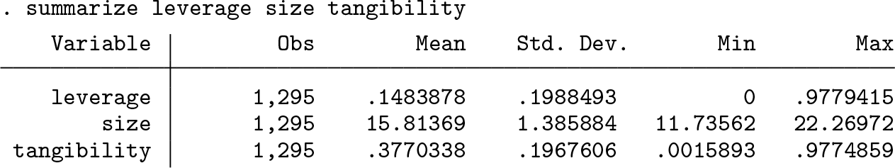
To illustrate the use of cmp, I rely on data from the study on financial leverage decisions by Ramalho and da Silva (2009). The data are available for download in a .txt fileformat at http://home.iscte-iul.pt/∼jjsro/data_code/ER-2015.txt and can be loaded into Stata by using import delimited. The dataset contains information on several firm characteristics. For this example, I will rely on leverage (long-term debt to long-term capital assets), size (natural logarithm of sales), and tangibility (sum of tangible assets and inventories divided by total assets). A complete description of the data is available in Ramalho and da Silva (2009).

First, I generate a nonzero indicator variable indicating the firms that have issued debt. To simplify the syntax, I assign the regressors to a global macro. I exclude the size variable from the list because we are going to use it as an exclusion restriction below. Valid exclusion restrictions are notoriously hard to come by, and this example is not different. By using size as an exclusion restriction, we are assuming that firm size is directly related to the participation decision but only related to the amount decision through the participation decision. In other words, firm size does not directly affect the proportion of debt sought by firms. While this assumption may be questionable, it will do for the purpose of this illustration.

3.2 Model estimation strategy

Some readers might have noticed how the GTP-FRM looks conceptually similar to the Heckman (1976) sample-selection model. In fact, the GTP-FRM is also applicable to fractional missing-data problems (Schwiebert and Wagner 2015). In the current setting, however, we do not have a sample-selection issue. Instead, we have a fractional response where the FDV is always observed yet is generated by two different dependent processes.

Conveniently, we can exploit the similarities to the sample selection model by using the same approach to fit the GTP-FRM. We do this by estimating systems of equations with errors that are jointly normally distributed. If our FDV had been binary, this estimation could have been performed using the heckprobit command. Because cmp allows for QMLE with a probit link, we can use cmp to estimate our parameters from the participation and magnitude equations simultaneously while obtaining an estimate of and accounting for ρ. In this way, cmp allows the participation and decision equations to vary by observation and enables consistent and efficient estimation. Thus, the estimation procedure becomes similar to that of the heckprobit command.

3.3 Syntax

The syntax for cmp is thoroughly described in Roodman (2011) and the cmp help file. Thus, in line with the aim of this article, I focus on its application to GTP-FRMs.

The cmp setup subcommand defines global macros that we use in the command line. In the command line, I specify the two equations, using size as an exclusion restriction in the participation equation. In indicators(), I specify the fractional probit using cmp frac and the regular probit using cmp probit. Note that I multiply cmp frac by the nonzero indicator variable, s. I use quietly to suppress most model output.

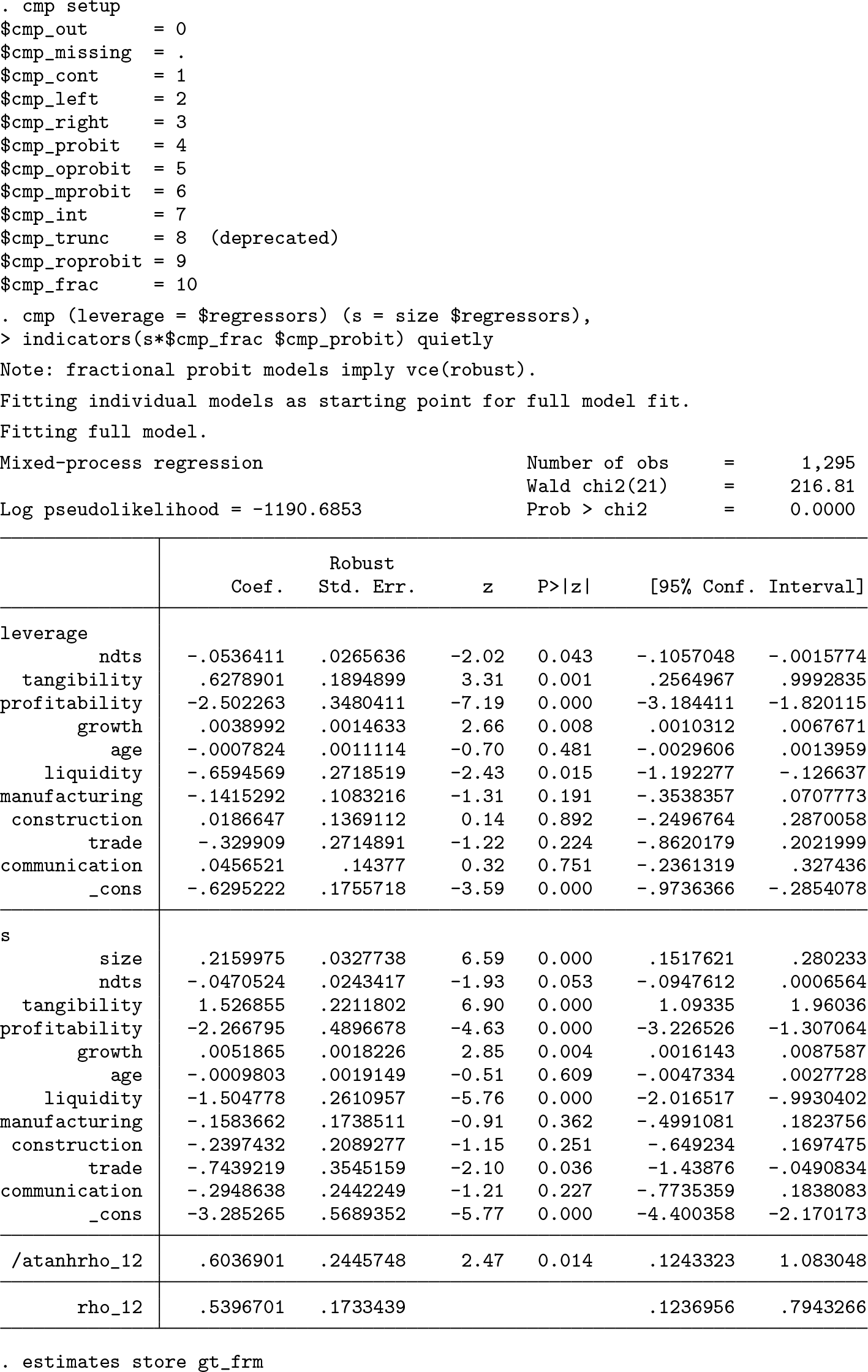
The first part of the output relates to the amount decision (leverage), while the second part of the output refers to the participation decision (s). The chosen estimation strategy provides a direct estimate of arctanh ρ = (1/2) ln{(1 + ρ)/(1 + ρ)}. Automatically, a Wald test is performed rejecting the regular TP-FRM at α = 0.05. Thus, a comparison with the TP-FRM is already incorporated in the procedure. Finally, we observe that the estimate of ρ is around 0.5. Thus, the Heckman-type estimation makes it possible to estimate the magnitude of the dependency between the two processes.

For illustration, we can compare the GTP-FRM estimates with those of the TP-FRM and regular FRM by using esttab (Jann 2005):

In the cmp output, we can observe a positive and significant association between tangibility and the amount decision. However, the corresponding estimate from the TP-FRM is substantially smaller and nonsignificant. In the FRM column, we can observe the impact of ignoring the two-part process. In this model, the estimated coefficient on tangibility is larger than the corresponding estimate in the second part of the two-part models because it “mixes” the coefficients from the two processes.

3.4 Predictions and marginal effects

To substantially interpret the results from the GTP-FRM, we can compute the (average) predicted proportions at selected values of tangibility using margins and plot them using marginsplot. In expression(), we specify the conditional expectation as shown in (3). Here, the first part is the predicted proportion of debt conditional on having debt, and the second part is the predicted probability of issuing debt.

Figure 1 shows the average predicted proportion of debt for various levels of firm profitability. At a tangibility around 0, the GTP-FRM predicts a debt proportion around 0.08. For firms with a higher ratio of tangible to total assets, the model predicts a dramatically higher debt proportion. For instance, for firms with roughly equal parts of tangible and intangible assets, the GTP-FRM predicts an average debt proportion of around 0.16.

Figure 1.

Marginsplot with predicted proportions

For computation of the average marginal effect on the conditional mean of leverage, we can invoke the dydx() option:

We can observe that a one-unit increase in tangibility is associated with an average increase in the proportion of debt by about 0.19. This estimate is significant at conventional alpha levels.

By slightly modifying the syntax above, we can quite easily obtain other types of predictions if we wish. For instance, we can compute the average marginal effect on the predicted probability of issuing debt by specifying only the predict(pr equation(s)) option:

A one-unit increase in tangibility is associated with a 0.54 average increase in the probability of issuing debt.

Finally, we can compute the average marginal effect on the proportion of debt conditional on the firm having issued debt:

The estimated average marginal effect is much smaller than the one on the conditional mean and is nonsignificant. This suggests that for firms that have issued debt, tangibility matters little for how much debt they choose to issue.

3.5 Model fit

While the procedure illustrated above automatically yields a test comparing the GTPFRM with the TP-FRM, we may want to compare the GTP-FRM with other specifications. Using (5) and (6), we can compare the GTP-FRM with any fractional specification we like. For instance, we can compare the GTP-FRM with the much simpler FRM specification:

The AIC and BIC values indicate that the GTP-FRM is not improving its fit enough to make up for its added complexity. Thus, it would seem that the FRM provides a better tradeoff between parsimony and fit than the GTP-FRM. As explained above, we can use this procedure to compare any model for the conditional mean as long as we can obtain RSS on the fractional scale.

3.6 RESET test

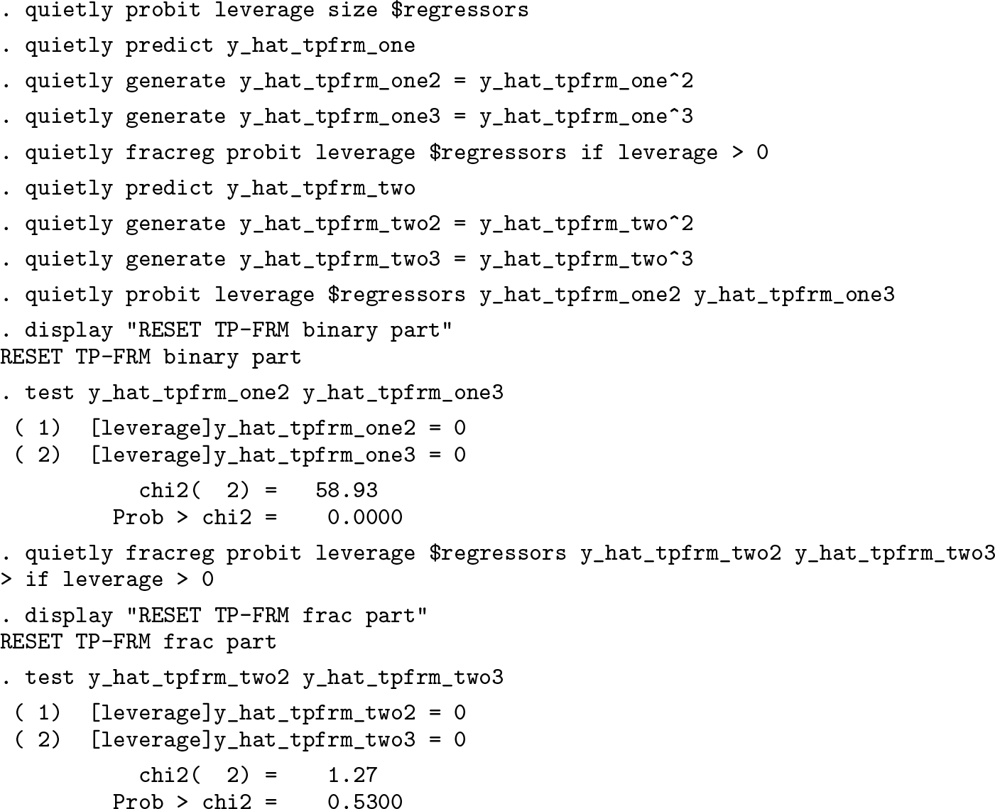
For testing the conditional mean specification, we can implement the RESET test. This can be done for each part separately by using the following procedure:

At an alpha of 1%, neither test rejects the H ₀ that the model specification is correct. In contrast, the RESET test rejects the H ₀ that the first part of the TP-FRM with a probit link is correctly specified:

4 Conclusion

FDVs are often modeled by researchers across many disciplines. When such variables are best described by a two-part process with dependence, researchers should apply the GTP-FRM. Currently, no dedicated Stata command exists to fit the GTP-FRM. In this article, I showed how GTP-FRMs can be fit with the community-contributed cmp command. Using a data example on the financial leverage of firms, I demonstrated how Stata users can fit GTP-FRMs and compute predictions, marginal effects, information criteria, and the RESET test statistic. Thus, the cmp command is useful for fitting fractional responses generated by two dependent processes.

Supplemental Material

Supplemental Material, st0558 - Generalized two-part fractional regression with cmp

Supplemental Material, st0558 for Generalized two-part fractional regression with cmp by Jesper N. Wulff in The Stata Journal

References

Aabo

Eriksen

N. B.

2018. Corporate risk and the humpback of CEO narcissism. Review of Behavioral Finance 10: 252–273.

Belotti

Deb

Manning

W. G.

Norton

E. C.

2015. twopm: Two-part models. Stata Journal 15: 3–20.

Cook

D. O.

Kieschnick

McCullough

B. D.

2008. Regression analysis of proportions in finance with self selection. Journal of Empirical Finance 15: 860–867.

Heckman

J. J.

1976. The common structure of statistical models of truncation, sample selection and limited dependent variables and a simple estimator for such models. Annals of Economic and Social Measurement 5: 475–492.

Jann

2005. Making regression tables from stored estimates. Stata Journal 5: 288–308.

Pagan

Vella

1989. Diagnostic tests for models based on individual data: A survey. Journal of Applied Econometrics 4: S29–S59.

Papke

L. E.

Wooldridge

J. M.

1996. Econometric methods for fractional response variables with an application to 401(K) plan participation rates. Journal of Applied Econometrics 11: 619–632.

Ramalho

E. A.

Ramalho

J. J. S.

2012. Alternative versions of the RESET test for binary response index models: A comparative study. Oxford Bulletin of Economics and Statistics 74: 107–130.

Ramalho

E. A.

Ramalho

J. J. S.

Murteira

J. M. R.

2011. Alternative estimating and testing empirical strategies for fractional regression models. Journal of Economic Surveys 25: 19–68.

10.

Ramalho

J. J. S.

da Silva

J. V.

2009. A two-part fractional regression model for the financial leverage decisions of micro, small, medium and large firms. Quantitative Finance 9: 621–636.

11.

Ramsey

J. B.

1969. Tests for specification errors in classical linear least-squares regression analysis. Journal of the Royal Statistical Society, Series B 31: 350–371.

12.

Roodman

2011. Fitting fully observed recursive mixed-process models with cmp. Stata Journal 11: 159–206.

13.

Sartori

A. E.

2003. An estimator for some binary-outcome selection models without exclusion restrictions. Political Analysis 11: 111–138.

14.

Schwiebert

Wagner

2015. A generalized two-part model for fractional response variables with excess zeros. Beiträge zur Jahrestagung des Vereins für Socialpolitik 2015: Ökonomische Entwicklung B04–V2. https://www.econstor.eu/handle/10419/113059.

15.

Wooldridge

J. M.

2010. Econometric Analysis of Cross Section and Panel Data. 2nd ed. Cambridge, MA: MIT Press.

16.

Wulff

J. N.

2015. Interpreting results from the multinomial logit model: Demonstrated by foreign market entry. Organizational Research Methods 18: 300–325.

17.

Wulff

J. N.

Villadsen

A. R.

2018. The use of tobit regression for modelling proportions and percentages in international business research. Aarhus University Business Statistics, Working Paper.

Supplementary Material

Please find the following supplemental material available below.

For Open Access articles published under a Creative Commons License, all supplemental material carries the same license as the article it is associated with.

For non-Open Access articles published, all supplemental material carries a non-exclusive license, and permission requests for re-use of supplemental material or any part of supplemental material shall be sent directly to the copyright owner as specified in the copyright notice associated with the article.

0.00 MB