qmodel: A command for fitting parametric quantile models

Abstract

In this article, we introduce the qmodel command, which fits parametric models for the conditional quantile function of an outcome variable given covariates. Ordinary quantile regression, implemented in the qreg command, is a popular, simple type of parametric quantile model. It is widely used but known to yield erratic estimates that often lead to uncertain inferences. Parametric quantile models overcome these limitations and extend modeling of conditional quantile functions beyond ordinary quantile regression. These models are flexible and efficient. qmodel can estimate virtually any possible linear or nonlinear parametric model because it allows the user to specify any combination of qmodel-specific built-in functions, standard mathematical and statistical functions, and substitutable expressions. We illustrate the potential of parametric quantile models and the use of the qmodel command and its postestimation commands through realand simulated-data examples that commonly arise in epidemiological and pharmacological research. In addition, this article may give insight into the close connection that exists between quantile functions and the true mathematical laws that generate data.

1 Introduction

The interest in modeling quantiles, such as the median and the 90th percentile, of a variable of interest given a set of covariates has spurred research in many fields of science. Applications and new methods have been increasingly appearing in the literature (among others, Koenker et al. [2018]). Quantile regression is arguably the most popular method for modeling conditional quantiles given covariates. The qreg command was released early on, and related commands such as qreg2, lqreg, and laplacereg have since been developed (Machado, Parente, and Santos Silva 2011; Orsini and Bottai 2011; Bottai and Orsini 2013).

Quantile regression can estimate a conditional quantile at a time, imposing no restrictions on the quantile function but on the assumed functional relationship between quantile and regression coefficients. For example, linear quantile regression assumes that a given quantile (for example, median) is a linear combination of covariates and unknown regression coefficients. While this gives ordinary quantile regression flexibility, it can also cause high variability of its estimator. Erratic estimates occur frequently in applications and often lead to uncertain inferences. For example, the coefficient at one percentile may be significantly different from zero, while those at adjacent percentiles are not; the induced quantile function may be decreasing for some covariate patterns; the estimated interquartile range may be smaller than the 20th-to-80th-percentile range.

In this article, we introduce the qmodel command, which fits parametric quantile models. The latter extend modeling of conditional quantile functions far beyond ordinary quantile regression. By specifying parametric forms, they can improve efficiency and ease interpretation at the possible cost of introducing bias (Frumento and Bottai 2016, 2017; Bottai and Cilluffo 2017). The qmodel command can fit parametric quantile models, allowing for most general specifications of conditional quantile functions given covariates, of which ordinary linear quantile regression and nonlinear quantile regression are special cases.

As a motivating example, we now introduce a simple linear parametric quantile model, on which we further elaborate in section 3. We analyze data from 930 subjects over 20 years old and with body mass index (BMI) over 30 kg/m² from the 2017 U.S. National Health and Nutrition Examination Survey (NHANES). Figure 1 shows the box plots of BMI over age groups. The bottom quantiles (for example, the 10th percentile) do not vary with age, while the top quantiles (for example, the 90th percentile) decline steeply.

Figure 1.

Box plots of BMI over age groups with data from NHANES

We define a model for the conditional quantile function of BMI given age

$Q(p|age) ={\beta }_0(p)+{\beta }_1(p)(age-\text{20})$

For example, Q(0.5|20) represents the conditional median in 20-year-old individuals. qreg can estimate the parameters β ₀(p) and β ₁(p) for any given quantile p ∊ (0, 1). We use it to estimate all the percentiles, Q(0.01|age), … , Q(0.99|age).

Figure 2 displays the regression coefficient estimated with both ordinary quantile regression and a parametric quantile model. The top row shows the estimated intercept, β ₀(p), and coefficient for age, β ₁(p), as functions of p, along with shaded areas indicating their 95% confidence intervals. The inclusion criteria explain the vanishing confidence intervals at the smallest quantiles. The estimates show a markedly erratic behavior, which can be explained only by sampling variability.

Figure 2.

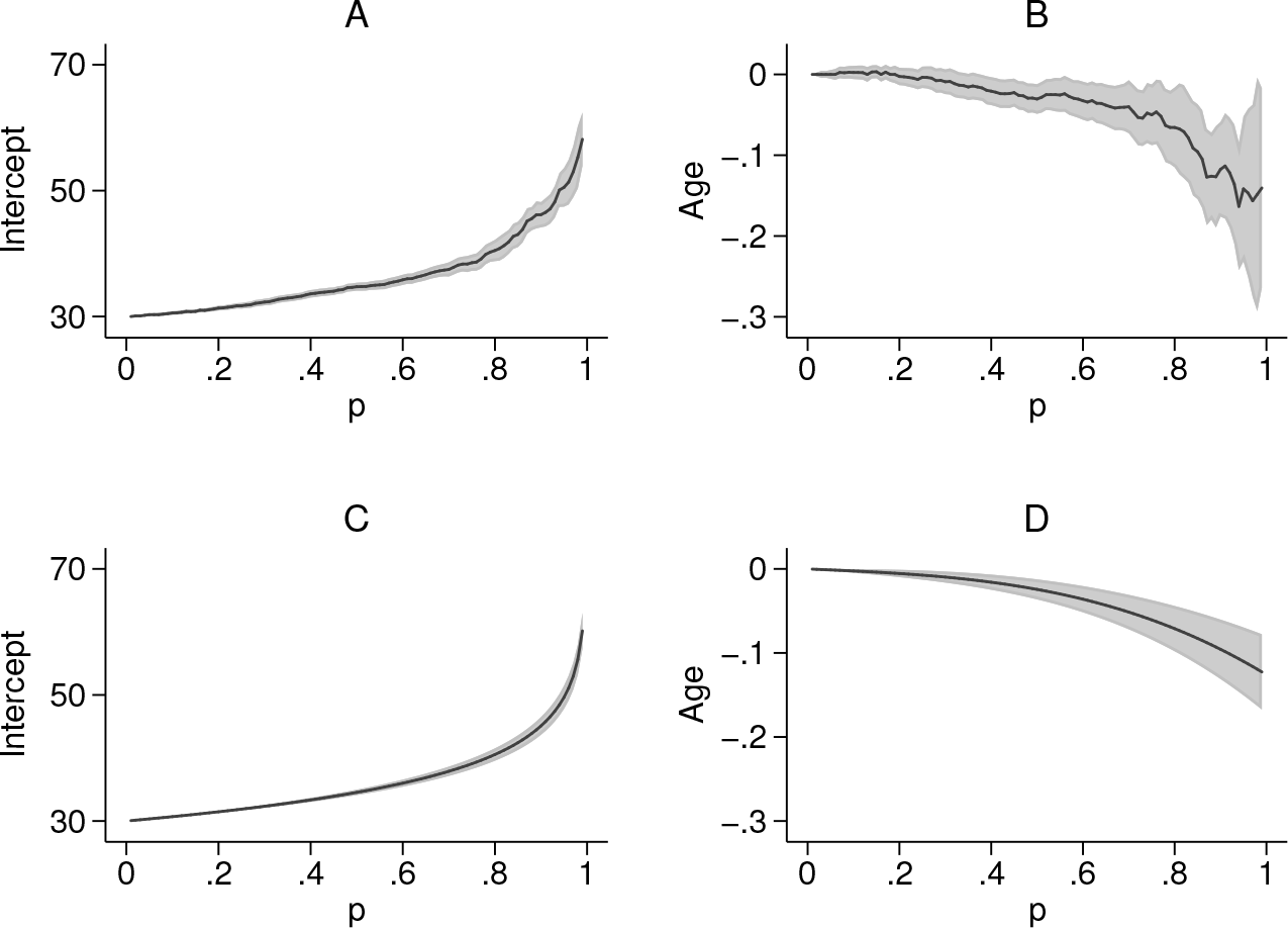
Point estimates (lines) and 95% confidence intervals (shaded areas) for the intercept (first column) and the coefficient for age (second column) from ordinary quantile regression (first row) and from the parametric quantile model (second row) as functions of the order of the quantile, p, with data from NHANES

The bottom row in figure 2 shows the estimates for the intercept and the coefficient associated with age obtained with a parametric quantile model. These can be compared with the 99 percentiles, Q(0.01|age),…, Q(0.99|age), shown in the top row, that were obtained with qreg. Although the overall trends are comparable, the parametric estimates are smoother, and their confidence intervals are narrower than their nonparametric counterparts.

The above is an example of a simple parametric quantile model. In the remainder of this article, we illustrate the potential of parametric quantile models. Section 2 contains the syntax of the qmodel command and its postestimation commands; section 3 expands on the example from the NHANES epidemiological study introduced above; section 4 describes a nonlinear parametric quantile model arising from an example of pharmacological modeling; section 5 provides additional details on parametric quantile models; and section 6 concludes with final remarks.

2 Syntax

This section describes the syntax of the qmodel command and its postestimation commands predict, qmodel plot, and qmodel quantile.

2.1 qmodel

qmodel fits parametric models for conditional quantile functions given covariates by minimizing the definite integral between 0 and 1 of the quantile loss function with respect to the order of the quantile, p.

exp varname is the variable whose quantile function is modeled or an expression of it such as log(varname) and logit(varname).

quantile function is an expression representing the parametric quantile model. It can be any combination of built-in functions, substitutable expressions, and mathematical functions. Its argument is indicated by the letter p. For example, the standard exponential quantile function is -log(1-p).

Options

cluster(varname) specifies the cluster variable used in the cluster–robust sandwich estimator for the standard errors.

npoints(integer) specifies the number of equally spaced internal points for the numerical integration. The default is npoints(99), which results in the following set of points: 0.01, 0.02,…, 0.99.

qpoints(numlist) specifies a list of points for the numerical integration. For example, qpoints(.05 .1(.1).9 .95). If both qpoints() and npoints() are specified, npoints() is ignored.

initial(values) specifies the initial values of the parameters for the optimization algorithm. The values are separated by commas. The default is a vector of zeros. The initial values correspond to the parameters in the order they appear in the quantile model expression quantile function. For example, initial(10, 0, -1).

log shows the iteration log.

Built-in functions

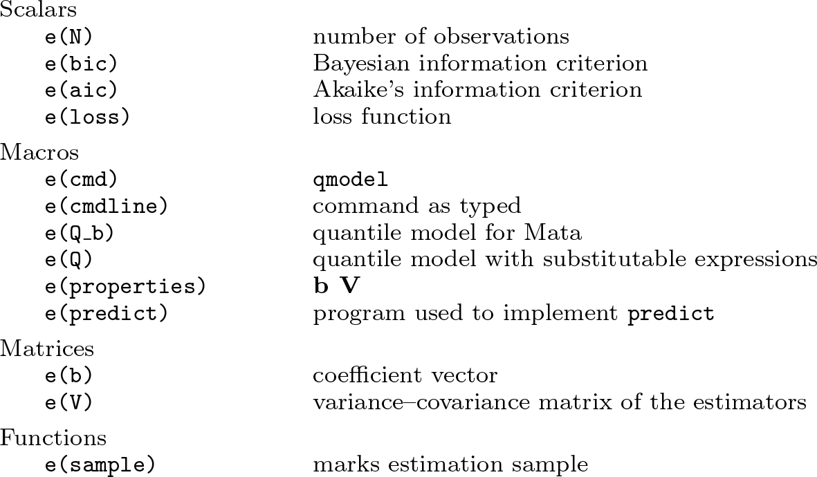
Stored results

qmodel stores the following in e():

2.2 predict

The predict command predicts specified functions of parameters at the proportions stored in the existing variable specified in proportion(varname). The functions of parameters to be predicted are specified in quantile function of qmodel using the special symbols _( and )_ or, equivalently, _[ and ]_. Standard errors of the predicted quantiles can be obtained with the se option.

Options

proportion(varname)specifies the name of an existing variable containing proportions. proportion() is required.

se specifies the standard error of the prediction.

2.3 qmodel plot

The qmodel plot command plots specified functions of the parameters against the proportion. The functions of parameters to be predicted are specified in quantile function of qmodel using the special symbols _( and )_ or, equivalently, _[ and ]_.

Options

ci shows confidence intervals of the quantiles.

replace replaces previous graph.

addplot(string) adds other plots to the generated graph.

twoway options are any of the options documented in [G-3] twoway options .

2.4 qmodel quantile

The qmodel quantile command computes point estimates, standard errors, test statistics, significance levels, and confidence intervals for the quantile of exp varname in qmodel at the proportions specified in numlist. The default is the median.

Options

at(varname = # [varname = # […]]) specifies the values of the covariates at which the quantiles are to be estimated.

nlcom options specifies standard nlcom options; see [R] nlcom.

3 Example 1: Body mass and age

In this section, we describe the use of the qmodel command and its postestimation commands. We expand on the simple linear regression model introduced in section 1. We present an example of nonlinear models in section 4.

The data arise from all the male participants in the 2017 NHANES who were at least 20 years old and had a BMI of at least 30 kg/m². We consider the simple linear regression model introduced in section 1,

$Q(p|age)={\beta }_0(p)+{\beta }_1(p)(age-20)$

The variable age is centered at the value 20, the smallest observed value in our data. The β ₀(p) function therefore represents the quantile function of BMI in 20-year-olds, that is, Q(p|20) = β ₀(p). We generally recommend ensuring that the value zero is within the observed range of all covariates because this eases the interpretation of the intercept function and the numerical stability of the estimation algorithm.

To construct parametric models for the regression coefficients, β ₀(p) and β ₁(p), one can obtain point estimates for a set of proportions with ordinary quantile regression, as shown in the top panels of figure 2, and then find a parametric quantile model that most closely approximates them.

Based on panel A in figure 2, we start by approximating the quantile function β ₀(p) with the quantile function of an exponential distribution with support BMI ≥ 30,

${\beta }_0(p)=30-{\theta }_0\hspace{0.17em}log(1-p)$

with θ ₀ > 0. Because the individuals were included in the study if their BMI was at least 30 kg/m², the smallest BMI value is known to be 30 with no sampling variability. Hence, we do not include a parameter representing a location shift of the baseline value but rather the fixed number 30.

We chose an initial approximating function for β ₀(p) based on the estimates for the intercept of ordinary quantile regression. If these were unavailable, we could consider the quantile function of BMI within a range of small age values. For example, we build the empirical quantile function of BMI in individuals between 20 and 25 years of age shown in figure 3.

Figure 3.

Empirical quantile function of BMI in individuals between 20 and 25 years old with data from NHANES

□ Technical note

The quantile function of a variable is its cumulative distribution function, where the x axis and y axis are swapped. The quantile function maps from the proportion (x axis) to the values of the outcome variable (y axis). □

When no graphical representations are available, one can start with flexible models such as cubic splines or step functions. Understanding the substantive meaning of the outcome variable can help one make sound decisions. For example, in our model, β ₀(p) represents the top tail of the conditional distribution of BMI truncated at 30 kg/m². While the exponential function would not be a reasonable choice for the entire distribution of BMI, which may be expected to be unimodal, it is a sensible initial approximation for its extreme top tail.

We now consider the regression coefficient associated with age, β ₁(p). Based on panel B in figure 2, we start by approximating it with a third-order polynomial with no intercept,

${\beta }_1(p)={\theta }_{1}p+{\theta }_2{p}^2+{\theta }_3{p}^3$

Other flexible functions, such as splines or step functions, could be used instead.

The quantile parametric model resulting from the above specifications is

$Q(p|age)=30-{\theta }_0\text{ log}(1-p)+({\theta }_{1}p+{\theta }_2{p}^2+{\theta }_3{p}^3)(age-20)$

The above model constrains the smallest BMI value to be equal to 30 kg/m², Q(0|age) = 30, at all age values, in accordance with the inclusion criterion BMI ≥ 30 kg/m².

We estimate the parameters of the above model with the qmodel command:

The table reports the estimates for all the model parameters along with their standard errors, z statistics, p-values, and 95% confidence intervals. The level of the confidence intervals can be changed with the set level command. The header above the table shows the value of the loss function, the number of observations used in the estimation, and the values of Akaike’s information criterion and the Bayesian information criterion.

The qmodel command in the above paragraph contains the following built-in functions: _exponential, _p, _p2, and _p3. The complete list of functions, each with a short description and its expanded expression, is given in section 2 and in the help files that open with the help qmodel command.

The built-in functions are internally expanded into standard substitutable expressions. qmodel saves the expanded syntax in the e(Q) macro, which can be retrieved as follows:

Typing the following command would give identical output to the above. For brevity, we suppress the output with the quietly command.

The model parameters are named within curly brackets. The letter p is the symbol that represents the proportion p, the argument of the quantile function Q(p). Any occurrences of the symbol p in the model expression are interpreted as such, so if a covariate named or abbreviated as p is included in the model, it is interpreted as the proportion, not the covariate. Similarly, if a covariate named or abbreviated as one of the built-in functions is included in the model, it is interpreted as the function, not the covariate. To introduce such a covariate, one needs to rename it first.

qmodel allows one to specify any function of parameters, covariates, and the proportion p. Curly bracket syntax, qmodel built-in functions, and Stata standard functions can be used in any combination, as demonstrated in the following sections and in the help documentation.

□ Technical note

The exponential built-in function constrains its mean to be positive by estimating the logarithm of the mean, which can take on any real value. This is a popular method for constraining parameters that must be positive. It ensures positive estimates for the mean and often improves the performance of the estimation algorithm. □

The above qmodel command specifies the qpoints(200) option, which increases the quadrature points in the estimation algorithm to 200. With the default 99 quadrature points, the algorithm fails to converge because the functions p ² and p ³ are nearly collinear over the interval p ∈ (0, 1).

The quadratic term of the coefficient for age is not significant, and we omit it from the model.

After we remove the quadratic term from the model, the near collinearity among covariates vanishes, and specifying the qpoints(200) option becomes unnecessary.

We now check the goodness of the fit of the exponential function by fitting the more flexible Weibull function, of which the exponential is a special case. We use the qmodel command with the built-in Weibull function:

The logarithm of the shape parameter of the Weibull quantile function is not significantly different from zero, which is equivalent to stating that the shape parameter is not significantly different from one. A Weibull distribution with shape equal to one is an exponential distribution. We therefore opt for the exponential quantile function. The values of Akaike’s information criterion and the Bayesian information criterion with the exponential function are smaller than those with the Weibull, further supporting our decision.

□ Technical note

Akaike’s information criterion and the Bayesian information criterion are often used to compare parametric quantile models that are nonnested. Although they are widely accepted, they are not always reliable and should generally be regarded as guidelines (Burnham and Anderson 2004). □

We consider the model with the exponential intercept our final model. It can be written as

$Q(p|age)=30-{\theta }_0\text{ log}(1-p)+({\theta }_{1}p+{\theta }_2{p}^3)(age-20)$

Its estimates for the functions β ₀(p) = 30 − θ ₀ log(1 − p) and β ₁(p) = θ ₁ p + θ ₂ p ³ are displayed on the bottom row of figure 2.

□ Technical note

The above final model sets the conditional distribution of BMI among 20-year-olds to be exponential, Q(p|20) = 30 − θ ₀ log(1 − p), with mean equal to θ ₀ and support over the half line (30, ∞). For increasing values of age, the conditional distribution smoothly morphs into a sequence of different distributions that are progressively farther away from the exponential. Their quantile function is the weighted sum of an exponential function and a cubic function, with weights varying with age. Except at age equal to 20 years, the corresponding conditional cumulative distribution function and conditional probability density function do not have a closed-form expression. Attempting to estimate the model parameters by maximizing the likelihood function would therefore be cumbersome. □

3.1 The qmodel plot command

This and the following two subsections describe the three postestimation commands of qmodel: qmodel plot, predict, and qmodel quantile.

The qmodel plot postestimation command produces plots for any sets of parameters specified in the latest qmodel command. We use qmodel plot to build the two plots on the bottom row of figure 2. To plot the β ₀(p) function, qmodel plot requires identifying the set of parameters that define the function to be plotted. This is accomplished by enclosing the relevant part of the qmodel command within the pair of special brackets _( and )_ . Square brackets _[ and ]_ can be used instead.

If the function to be plotted is specified by the special brackets in the qmodel command, as above, we can use the qmodel plot command to plot it.

Panel C in figure 2 shows the resulting plot. The ci option requires pointwise confidence bands to be laid over the point estimates. The standard two-way plot options, such as ylabel() and ytitle(), are allowed. We refer the reader to the documentation of the twoway command for more details.

The special brackets in the qmodel command are required only for later qmodel plot commands, which need them to identify the functions to plot. The qmodel command itself does not need them, as demonstrated in the examples presented in the first part of section 3.

We now use the qmodel plot command to plot the β ₁(p) function shown in panel D in figure 2 after enclosing this function within special brackets in the qmodel command.

When multiple sets of special brackets are included, the qmodel plot command produces multiple graphs. For example, the following two lines of code produce the above two plots simultaneously (graphs not shown in this article).

When multiple graphs are specified, these are given default names, and the name() option is not allowed. Any options specified in the qmodel plot command would apply to all the graphs.

As noted in section 1, the overall trend of the parametric and nonparametric estimates are similar, the former are smoother, and their confidence intervals narrower than the latter. The confidence intervals vanish as the proportion p tends to 0 because of the inclusion criterion BMI ≥ 30 kg/m².

3.2 The predict command

The predict command predicts specified functions of parameters and their standard errors at values of p stored in an existing variable, specified by the required proportion() option. For example, we estimate the 99 percentiles after generating a new variable named proportion that contains the proportions 0.01 to 0.99 by 0.01 steps. We also estimate the corresponding standard errors by specifying the se option.

The estimates for the quantiles are stored in the newly created variables named beta0 and beta1. The corresponding estimates for the standard errors are stored in the newly created variables named se beta0 and se beta1. Because the above qmodel command contains two sets of enclosed parameters, in the predict command, we specify two new variable names, one for each set of parameters. If only one variable name is provided, predict predicts only the first set of enclosed parameters given in the qmodel command. In general, if there are fewer new variable names listed in the predict command than the number of parameter sets, predict predicts only those specified in the order they appear in the model given in the qmodel command.

We list the estimates for the specified sets of parameters at the median, β ₀(0.5) and β ₁(0.5), with their respective standard errors.

Plotting the newly generated variables, beta0 and beta1, against the newly created variable proportion would produce the same plots as those created by the qmodel plot command, shown on the bottom row of figure 2.

3.3 The qmodel quantile command

The qmodel quantile command can estimate any quantiles at any specified covariate values from the latest qmodel command. For example, we estimate the median BMI in the 30-year-old male and obese NHANES population.

The above table shows the estimated quantile along with its standard error, z statistic, p-value, and 95% confidence intervals. The estimated median is 34.3 kg/m² with a standard error of 0.170 and a 95% confidence interval equal to [34.0, 34.6].

Above, we did not specify any proportion, and the qmodel quantile command defaulted to the median. The proportion can be specified as a numeric list. For example, we estimate the 95th, 96th, and 97th percentiles of BMI in 30-year-old individuals.

In our study population, the 95th percentile is estimated to be 48.5 kg/m² with a standard error of 0.753 and a confidence interval equal to [47.1, 50.0].

The above qmodel quantile command specifies the noheader option. The command is based on the nlcom command and allows all the options of that command. We refer the reader to the documentation of this command for more details.

Thanks to the parametric assumptions, we can obtain estimates for any percentile, however extreme. For example, we estimate the 0.9999 quantile as follows:

Our data contain only 930 individuals. This implies that the above estimate of 89.1 kg/m² is an extrapolation, valid only if the parametric quantile model is true. Ordinary quantile regression would be unable to estimate such an extreme percentile. As with any other statistical method, one should generally be cautious when interpreting extrapolated inferences.

4 Example 2: Nonlinear dose–response relationships

Parametric quantile models extend beyond the ordinary linear quantile regression framework. Some examples of the range of possibilities are described in section 5. This section describes the estimation of a nonlinear parametric quantile model frequently used in pharmacological research.

We analyze the data from a fictitious laboratory experiment in which 200 animals were injected with 5 doses of an agent, and 400 more animals were injected with the same 5 doses but of a different agent. The liver concentration of the agent was measured one hour after injection. Figure 4 shows the data and true conditional median of the liver concentration for the two agents.

Figure 4.

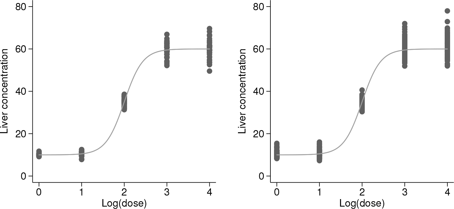
Observed liver concentration (dots) and true median concentration (line) at 5 injected doses of the first agent (left panel) and the second agent (right panel) with simulated data

In our data, the location, spread, and overall shape of the distribution of liver concentration change over dose and between agents. We consider a popular dose–response function, the Hill function,

$\text{concentration}={\theta }_0+\frac{{\theta }_1-{\theta }_0}{1 + {10}^{{\theta }_2}{\hspace{0.17em}}^{({\theta }_3-\text{dose})}}+\epsilon$

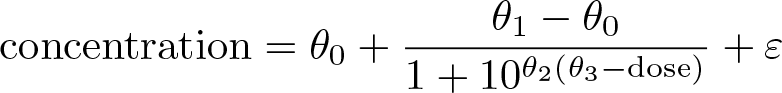
The parameters of the above model can be interpreted as follows: minimal response (θ ₀), maximal response (θ ₁), slope (θ ₂), and dose corresponding to half the maximal response (θ ₃). The error term, ε, is generally assumed to follow a normal distribution.

A possible specification of the Hill quantile function is

$Q(p|\text{dose})={\theta }_0+\frac{{\theta }_1-{\theta }_0}{1 + {10}^{{\theta }_2}{\hspace{0.17em}}^{({\theta }_3-\text{dose})}}+\epsilon (p)$

For the error term, we use the specification

$\epsilon (p)=\text{exp}({\theta }_4+{\theta }_5\text{dose})z(p)$

with the first injected agent and

$\epsilon (p)=\text{exp}({\theta }_4+{\theta }_5\text{dose})z(p) +{\theta }_6\{\text{log}(0.5)-\text{log}(1-p)\}$

with the second injected agent. The term z(p) denotes the standard normal quantile function.

The error term with the first agent follows a heteroskedastic normal distribution. With the second agent, the quantile function of the error term is the sum of a heteroskedastic normal quantile function and an exponential quantile function centered at the median. The two parameters θ ₄ and θ ₅ allow for the observed increasing variability of liver concentration and dose. The exponential function is applied to constrain the standard deviation of the error term to be positive. The parameter θ ₆ models the changing shape of the error distribution between agents.

Because ε(0.5) = 0, the conditional median concentration given dose is

$Q(0.5|\text{dose})={\theta }_0+\frac{{\theta }_1-{\theta }_0}{1 + {10}^{{\theta }_2}{\hspace{0.17em}}^{({\theta }_3-\text{dose})}}$

We generated the data shown in figure 4 with the following code:

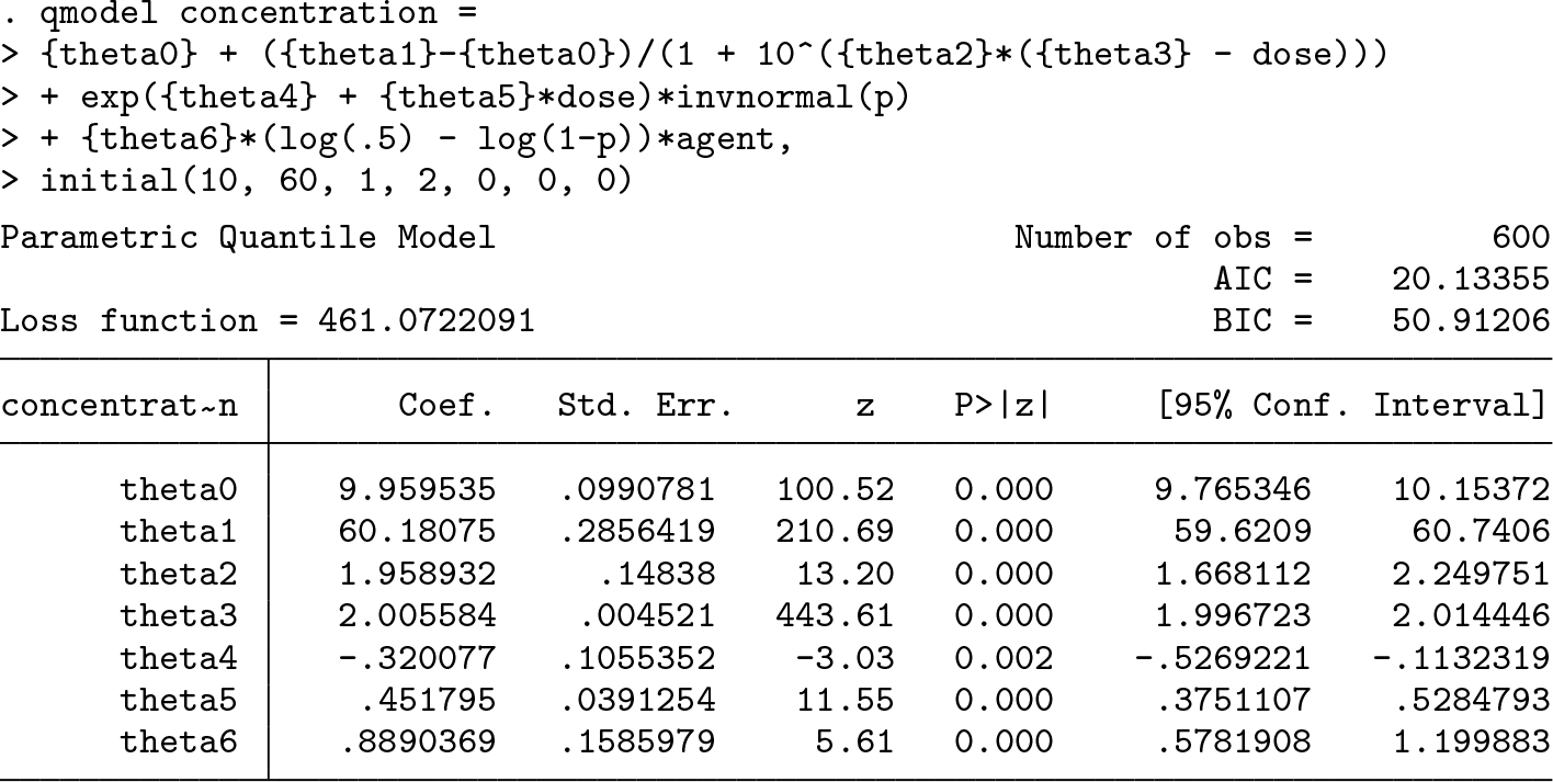
We use the qmodel command to estimate the parameters of the Hill quantile function only for the first agent.

The confidence intervals of all the parameters are approximately centered at the respective true values used in the above data-generating code, θ ₀ = 10, θ ₁ = 60, θ ₂ = 2, θ ₃ = 2, θ ₄ = −0.3, and θ ₅ = 0.4.

□ Technical note

The expression of the quantile function in the above qmodel command is the same as that used in the generate command in the simulation above, except that the parameters are replaced by numeric values in the latter command. This may help one see quantile functions as true data-generating laws. □

To facilitate convergence of the estimation algorithm, we specified the initial values of the parameters with the initial() option. Pretending not to know the true values, we determined the initial values as follows: based on visual inspection of figure 4, we set the minimal response θ ₀ = 10, the maximal response θ ₁ = 60, and the dose corresponding to half the maximal response θ ₃ = 2. The slope was assigned the value θ ₂ = 1, a reasonable positive number, and the variance parameters were assigned the values θ ₄ = 0 and θ ₅ = 0, corresponding to homoskedastic standard normal errors. If the initial values were not specified, the qmodel command would default to the initial value zero for all the parameters and fail to converge.

We now use the qmodel quantile command to estimate the median and 95th percentile of liver concentration at the control dose.

The estimated 95th percentile is equal to 11.2 mg/ml with a standard error of 0.2 and a 95% confidence interval equal to [10.8, 11.6].

Presently, no command can estimate ordinary quantile regression with nonlinear models (Koenker and Park 1996). We therefore compare the above estimates with those from the nl command, which can fit nonlinear models for the conditional mean of the outcome variable. Under the normal errors generated in our fictitious example with the first injected agent, the conditional median is identical to the conditional mean.

The above nl command also requires specifying the initial values of the parameters because not doing so would produce wrong estimates. Owing to the error of heteroskedasticity, we request the robust estimator for the standard errors.

Finally, we model the differences between the two injected agents with the qmodel command. We include the additional parameter θ ₆ to model the different shape of the error distribution between the two agents. We set the initial values for the parameters θ ₀ to θ ₅ as before. We set the initial value for the additional parameter θ ₆ equal to 0, corresponding to the case of equal error distribution with both agents.

The confidence intervals of all the parameters are approximately centered at the respective true values used in the above data-generating code. The true value for the additional parameter is θ ₆ = 1. With the second agent, the conditional median is different from the conditional mean, and the above estimates cannot be compared with those from the nl command.

All the qmodel commands in this section estimate the respective true quantile functions. These are known because we generated the data ourselves. In real-data settings, the true quantile functions obviously are unknown, and good-fitting models should be found. For brevity, however, we do not discuss model-building strategies in this section; some are described in section 3.

5 More details about parametric quantile models

This subsection contains further details about parametric quantile models and their potentials. Parametric quantile models were introduced by Frumento and Bottai (2016, 2017) and Bottai and Cilluffo (2017). See those articles for more information.

The conditional quantile function of an outcome variable of interest y given a k-dimensional vector of covariates x is defined as

$Q(p|x)=\text{inf}\{y:P(Y\le y|x)=p\}$

The symbol p ∊ (0, 1) represents the order of the quantile. For example, p = 0.5 corresponds to the conditional median. The function Q(p|x) is nondecreasing with respect to its argument, the proportion p.

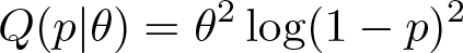
Parametric quantile models assume the quantile function to be known up to a parameter vector θ. For example, the quantile function of a variable uniformly distributed between zero and θ > 0 is

$Q(p|\theta )=\theta p$

and that of an exponential variable with mean equal to θ > 0 is

$Q(p|\theta )=-\theta \hspace{0.17em}\text{log}(1-p)$

Parametric quantile functions provide a flexible framework for modeling shapes of distributions because of their properties. First, they are invariant to monotone transformations of the outcome variable. For example, if Q(p) is the quantile function of a variable y, then

$g\{Q(p)\}$

is the quantile function of g(y) for any monotone function g : ℛ ↦ ℛ. For example, the quantile function of a variable whose square root is exponential with mean equal to θ is

$Q(p|\theta )={\theta }^2\text{log}{(1-p)}^2$

and that of a standard log-normal variable is

$Q(p|\theta )=\text{exp}\{z(p)\}$

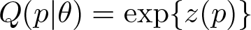
where z(p) indicates the standard normal quantile function.

Second, the modeling potential of parametric quantile models can be expanded by considering that sums, products, and functions of nondecreasing functions are themselves nondecreasing. For example, if two functions g ₁(p) and g ₂(p) are nondecreasing over the interval p ∊ (0, 1), then

$g_1(p)+g_2(p)$

is nondecreasing. If g ₁ is nondecreasing on the entire real line, then

$g_1\{g_2(p)\}$

is nondecreasing. If two functions g ₁(p) and g ₂(p) are nondecreasing and positive over p ∊ (0, 1), then

$g_1(p)g_2(p)$

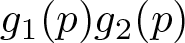
is nondecreasing.

The possible dependence of the quantile function on the covariates can be evaluated by including the covariates in the model. For example,

$Q(p|x_1, x_2)=\text{exp}({\theta }_0+{\theta }_1{x}_1+{\theta }_2{x}_2)p$

defines a uniform distribution with support between zero and a value that depends on the values of the two covariates x ₁ and x ₂;

$Q(p|x_1, x_2)=\text{log}(2p)-\text{exp}({\theta }_0+{\theta }_1{x}_1+{\theta }_2{x}_2)\text{ log}(2-2p)$

defines a unimodal, asymmetric, and zero-median logistic distribution whose variance and skewness depend on the covariate values; and

$Q(p|x_1,x_2) =t\{p|2+exp({\theta }_0+{\theta }_1{x}_1+{\theta }_2{x}_2)\}\sqrt{\frac{\text{exp}({\theta }_0+{\theta }_1{x}_1+{\theta }_2{x}_2)}{2+\text{exp}({\theta }_0+{\theta }_1{x}_1+{\theta }_2{x}_2)}}$

with t(p|ν) representing the quantile function of the Student’s t-distribution with ν degrees of freedom, defines a distribution whose kurtosis changes along with values of covariates, while the mean, variance, and skewness remain unchanged.

Ordinary quantile regression assumes

$Q(p|x_1, x_2)={\beta }_0(p)+{\beta }_1(p)x_1+{\beta }_2(p)x_2$

The above conditional quantile function is the weighted sum of three functions of p, β ₀(p), β ₁(p), and β ₂(p), with weights defined by the covariate values, x ₁ and x ₂.

All the above models can be fit with the qmodel command.

5.1 Transformations of the outcome variable

This subsection illustrates the potentials of transforming the outcome variable. The qmodel command easily allows one to model transformation of the outcome variable of interest. For example, we generate 1,000 random observations from a log-normal distribution and estimate its parameters with three alternative and equivalent syntax specifications.

The first syntax models log(y) with a normal distribution, the second models y with a log-normal distribution using the _lognormal built-in function, and the third models y applying the exponential function to the _normal built-in function. The estimates from the last two specifications are identical to each other. The estimates from the first slightly differ from the other two because of numeric approximations. The loss function of the first is substantially smaller in the first model specification because of the different scale of the outcome variables. The first syntax is often the most stable computationally, especially when the outcome variable takes on large values that cannot be exponentiated at double precision.

As a second example, we generate 1,000 random observations from a logit-normal distribution and estimate its parameters with three alternative and equivalent syntax specifications.

The logit normal is a flexible distribution for outcome variables that are bounded within a known interval, such as visual analogue scales and percentages. It constitutes an alternative to the beta distribution, which is implemented in the beta built-in function.

5.2 Sums of functions for modeling skewness and kurtosis

This subsection briefly introduces the use of sums of quantile functions as a flexible modeling tool. In particular, we discuss sums of functions for modeling skewness and kurtosis. As an example of a model for skewness, we consider a quantile function defined as the sum of a standard normal quantile function and a standard exponential quantile function. The left-hand-side panel shows the right-skewed histogram of the 1,000 generated observations. The quantile function is depicted by the thick line in the right-hand-side panel of figure 5. Its two components are shown as the solid thin line (standard normal) and the dashed thin line (standard exponential).

Figure 5.

Left-hand-side panel: histogram of 1,000 observations generated from a quantile function defined as the sum of a standard normal and standard exponential distribution; right-hand-side panel: the estimated quantile function (thick line) and its constituent parts, standard normal (solid thin line) and standard exponential (dashed thin line).

We generate 1,000 random observations and estimate the parameters with qmodel with the two built-in functions _normal and _exponential.

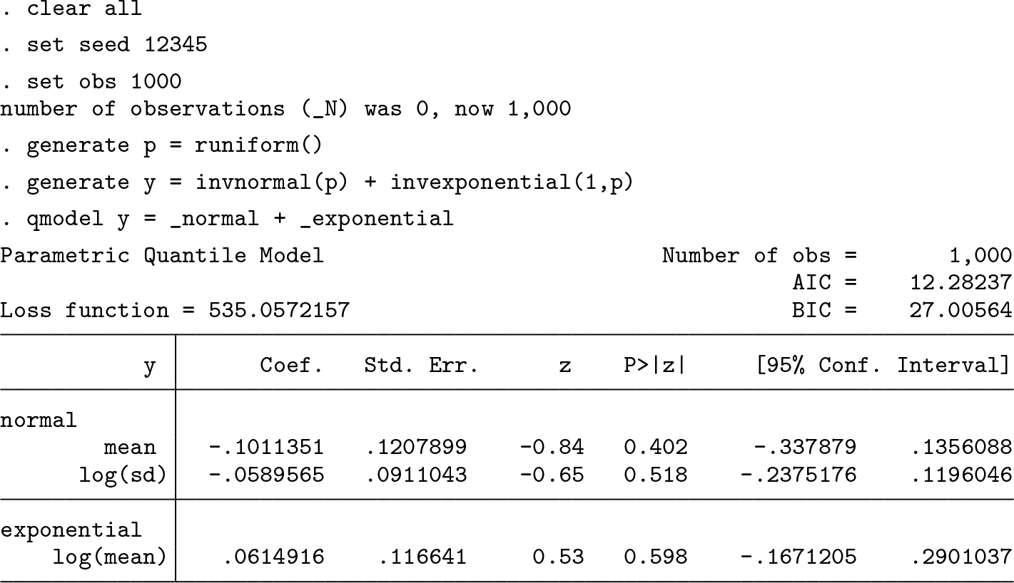
The estimated parameters are not significantly different from zero, which is their true value.

As an example of a model for kurtosis, we consider a quantile function defined as the sum of the standard normal quantile function and another standard normal raised to the third power. The left-hand-side panel shows the thick-tailed histogram of the 1,000 generated observations. The resulting quantile function is depicted as the thick line in the right-hand-side panel of figure 6. Its two components are shown as the solid thin line (standard normal) and the dashed thin line (standard normal cubed).

Figure 6.

Left-hand-side panel: histogram of 1,000 observations generated from a quantile function defined as the sum of the standard normal quantile function and another standard normal raised to the third power; right-hand-side panel: the estimated quantile function (thick line) and its constituent parts, standard normal (solid thin line) and the standard normal cubed (dashed thin line).

We generate 1,000 random observations and estimate the parameters with qmodel with the two built-in functions _normal and _cnormal:

All the confidence intervals contain their respective true values. With the same thick-tailed yet symmetric data as above, we fit a model with the three built-in functions _normal, _cnormal, and _clog:

The _clog built-in function is similar to _exponential except it does not constrain its parameter to be strictly positive. It therefore can model distributions skewed either to the left or to the right. Its estimated parameter is not significantly different from zero, which is its true value. The estimates of the other parameters in the model are close to those of the previous model, which did not allow for skewness.

5.3 Modeling conditional parametric quantile functions

This section illustrates the use of qmodel and its postestimation commands when the quantile function depends on a set of covariates. We generate 1,000 random observations from a quantile function defined as

$Q(p|x)=z(p)-x_1+x_2$

where z(p) represents the standard normal quantile function, x ₁ is a binary covariate with 0.5 probability, and x ₂ is a standard normal covariate. The above conditional distribution is normal with unit standard deviation and mean that depends on a linear combination of the two covariates.

We estimate the parameters with the two built-in functions _normal and _flat. The latter represents a flat or constant function of the proportion p. When the same built-in function is specified multiple times, qmodel enumerates them in the order they appear in the model.

All the estimates are close to the true values with which the data were generated. The estimates are similar to those from linear regression.

The data were generated with a homoskedastic error with standard deviation equal to 1. Hence, the true value of the logarithm of the standard deviation of the normal function in the quantile model is zero. The estimate from qmodel, −0.0063547, can be compared with that from regress.

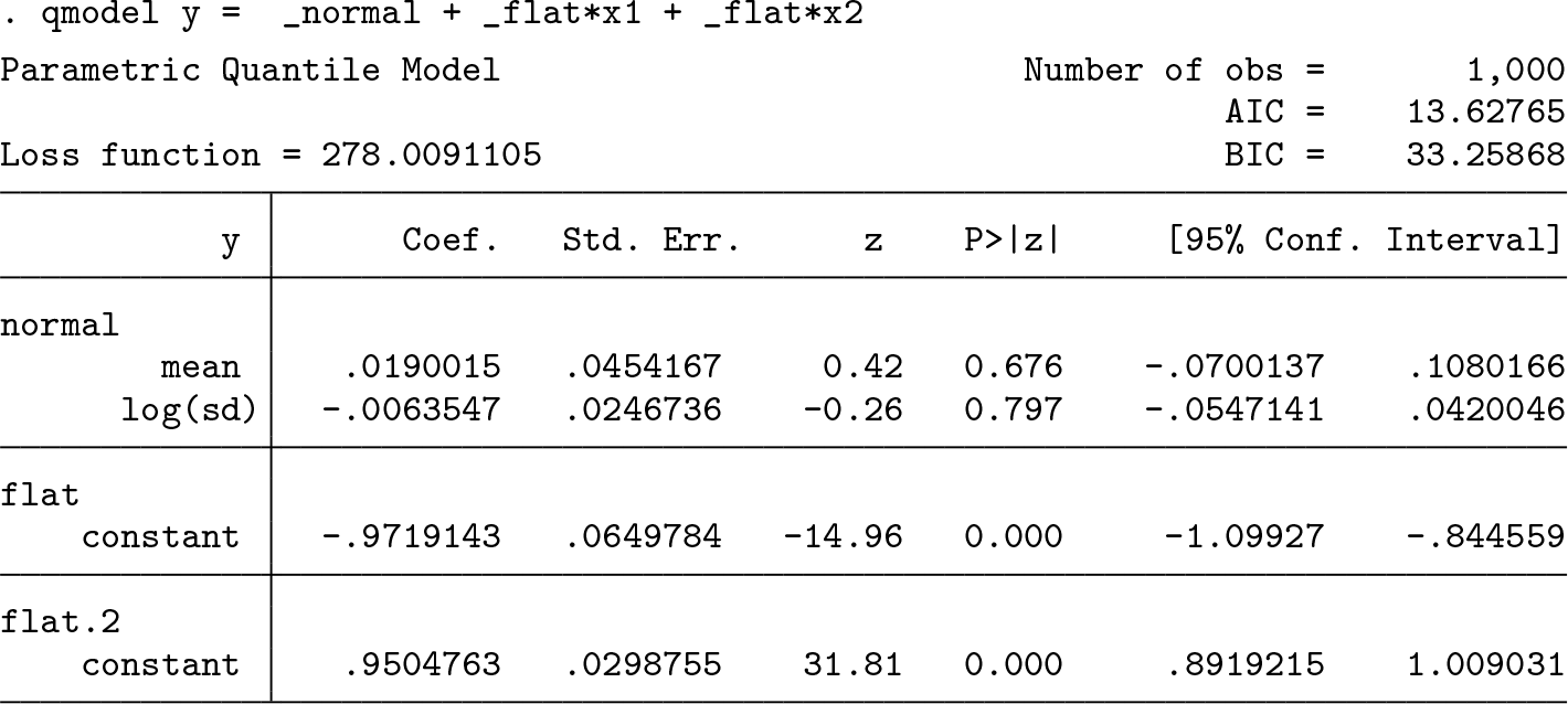
To help explain parametric quantile models and the qmodel command, we now fit a misspecified model in which the flat function for the covariate x ₂ is replaced by a normal quantile function.

The estimated mean of the normal for the coefficient of x ₂, 0.95, is close to the estimate for the flat function in the previous model, and its estimated standard deviation, exp(−14.5226) = 0.0000004931, is nearly 0. Therefore, the resulting function for the coefficient of x ₂ is essentially flat, which is the true shape under which the data were generated. The estimates of all the other parameters are nearly unchanged from the previous model, where the coefficient of x ₂ was correctly specified as a flat function.

5.4 Ordinary quantile regression as a special case of quantile models

Ordinary quantile regression can be seen as a special case of the more general parametric quantile models. For example, we estimate the conditional median of a variable y given a covariate x.

The above estimates are similar to those that can be obtained with the qreg command.

When the interest is only in the median and not in the entire quantile function, a computationally faster alternative is to specify only one quadrature point at 0.5 with the qpoints() option.

Any quantile can be estimated by specifying the corresponding proportion in the qpoints() option.

6 Final remarks

Parametric quantile models define the entire conditional distribution of the outcome variable of interest. If of interest, they can be used to generate simulated data, plot quantile functions and cumulative distribution functions by simply swapping the axes, plot probability density functions by differentiating the cumulative distribution function with the dydx command, and estimate treatment effects (Frölich and Melly 2010; Cattaneo, Drukker, and Holland 2013). The large- and small-sample behavior of the estimator of parametric quantile models is described by Frumento and Bottai (2016) for linear models, by Frumento and Bottai (2017) for linear models with censored and truncated data, and by Bottai and Cilluffo (2017) for nonlinear models. The qmodel command can provide estimates for conditional quantiles that are generally more efficient than those obtained by ordinary quantile regression. However, misspecified parametric models may yield biased estimates. Using the qmodel command requires careful model building. As illustrated in sections 3 and 4, one can avail oneself of visual representations and comparison of nested and nonnested parametric models with varying degrees of complexity. Frumento and Bottai (2016) presented an overall goodness-of-fit test based on the Kolomogorov–Smirnov’s test statistic.

Supplemental Material

Supplemental Material, st0555 - qmodel: A command for fitting parametric quantile models

Supplemental Material, st0555 for qmodel: A command for fitting parametric quantile models by Matteo Bottai and Nicola Orsini in The Stata Journal