Updates to the ipfraking ecosystem

Abstract

Kolenikov (2014, Stata Journal 14: 22–59) introduced the package ipfraking for iterative proportional fitting (raking) weight-calibration procedures for complex survey designs. In this article, I briefly describe the original package and updates to the core program and document additional programs that are used to support the process of creating survey weights in the author’s production code.

1 Introduction and background

Large-scale social, behavioral, and health data are often collected via complex survey designs that may involve stratification, multiple stages of selection, unequal probabilities of selection (Korn and Graubard 1995, 1999), or any combination thereof. In an ideal setting, one accounts for varying probabilities of selection by using the Horvitz– Thompson estimator of the totals (Horvitz and Thompson 1952; Thompson 1997), and the remaining sampling fluctuations can be further ironed out by poststratification (Holt and Smith 1979). However, on top of the planned differences in probabilities of obtaining a response from a sampled unit, nonresponse is a practical problem that has been growing more acute in recent years (Groves et al. 2002; Pew Research Center 2012). The analysis weights provided along with the public use microdata by datacollecting agencies are designed to account for unequal probabilities of selection, nonresponse, and other factors affecting imbalance between the population and the sample, thus making the analyses conducted on such microdata generalizable to the target population.

Earlier work (Kolenikov 2014) introduced the package ipfraking, which implements calibration of survey weights to known control totals to ensure that the resulting weighted data are representative of the population of interest. The process of calibration is aimed at aligning the sample totals of the key variables with those known for the population as a whole. The remainder of this section provides a condensed treatment of estimation with survey data using calibrated weights; I provided a full description in the previous article.

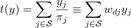
For a given finite population u of units indexed i = 1,…, N, the interests of survey statisticians often lie in estimating the population total of a variable Y :

$T(Y) ={\displaystyle \sum _{i\in \hspace{0.17em}u}{Y}_i}$

1

A sample S of n units indexed by j = 1,…, n is taken from u. If the probability to select the ith unit is known to be π_i , then the probability weights, or design weights, are given by the inverse probability of selection,

$w_{di}={\pi }_i^{-1}$

where subscript d stands for design probabilities of selection. With these weights, an unbiased (design-based, nonparametric) estimator of the total of (1), according to Horvitz and Thompson (1952), is

$t(y) ={\displaystyle \sum _{j\in \text{S}}\frac{y_j}{{\pi }_j}}\equiv {\displaystyle \sum _{j\in \text{S}}w{d}_j{y}_j}$

Probability weights protect the end user from potentially informative sampling designs in which the probabilities of selection are correlated with outcomes and relieve the user from the need to fully account for the sampling design variables in their analysis. This is required in methods such as multilevel regression with poststratification (Park, Gelman, and Bafumi 2004). Design-based methods generally ensure that inference can be generalized to the finite population even when the statistical models used by analysts and researchers are not specified correctly (Pfeffermann 1993; Binder and Roberts 2003).

Survey statisticians often have auxiliary information on the units in the frame, and such information can be included at the sampling stage to create more efficient designs. Unequal probabilities of selection are then controlled with probability weights, implemented as [pw= varname ] in Stata (and can be permanently affixed to the dataset with the svyset command; see [SVY] svyset).

In many situations, however, usable information is not available beforehand and may appear only in the collected data. For example, the census totals of the age and gender distribution of the population may exist, but age and gender of the sampled units are unknown until they are measured in the survey. One can still capitalize on this additional data by adjusting the weights in such a way that the reweighted data conform to these known figures. The procedures to perform these reweighting steps are generally known as weight calibration (Deville and Särndal 1992; Deville, Särndal, and Sautory 1993; Kott 2006, 2009; Särndal 2007).

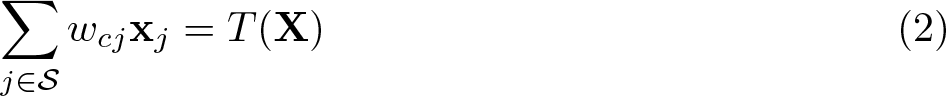
Suppose there are several variables, referred to as control variables, that are available for both the population and the sample (age groups, race, gender, educational attainment, etc.). Categorical variables are represented by the 0/1 category indicators, although Kolenikov and Hammer (2015) provide an illustrative example of how the counts of persons in each demographic category within a household (that is, variables taking values 0, 1, 2,…) can be used to create person-level weights that are constant within households. Weight calibration aims to adjust the weights via an iterative optimization so that the control totals for the control variables x _j = (x _{1 j},…, x_pj ), obtained with the calibrated weights w_cj , align with the known population totals:

${\displaystyle \sum _{j\in \text{S}}{w}_{cj}{x}_j}=T(X)$

2

The population totals of the control variables in the right-hand side of (2) are assumed to be known from a census or a higher quality survey. Deville and Särndal (1992) framed the problem of finding a suitable set of weights as that of constrained optimization with the control equations (2) serving as constraints. Optimization is targeted at making the discrepancy between the design weights w_dj and calibrated weights w_cj as close as suitably possible.

The package ipfraking (Kolenikov 2014) implements a popular calibration algorithm known as iterative proportional fitting, or raking, that consists of iterative updating (poststratification) of each of the margins. For an in-depth discussion of distinctions between raking and poststratification, see Kolenikov (2016). Since 2014, the continuing code development resulted in additional features that this update documents.

2 Updates to ipfraking program and package

Listed below is the full syntax of ipfraking. For a description of its options, see Kolenikov (2014).

2.1 Syntax for ipfraking

ipfraking [if] [in] [pw= varname ], ctotal( matrix_name [matrix_name…])

{ generate( newvar ) | replace} [ tolerance( # ) iterate( # ) nodivergence ctrltolerance( # ) trace alpha( # ) trimhiabs( # ) trimhirel( # ) trimloabs( # ) trimlorel( # ) trimfrequency(once| sometimes| often) double meta nograph loglevel( # ) linear]

2.2 New features of ipfraking

The new features of ipfraking concern reporting and diagnostics, an alternative functional form specification, and richer metadata stored in the characteristics of the weight variable.

Reporting of results and errors by ipfraking was improved in several ways. It now reports the discrepancy for the worst-fitting category and the number of trimmed observations.

Using example 3 from Kolenikov (2014) with trimming options, we have

If ipfraking determines that the categories do not match in the control totals received from ctotal()and those found in the data, it provides a full listing of categories and explicitly shows the categories not found in one or the other. Using example 2 of Kolenikov (2014), let us modify one of the variables to a nonsensical value:

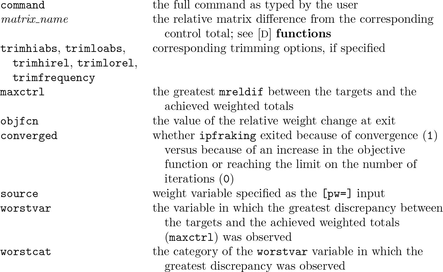
Option meta saves more information in characteristics of the calibrated weight variables that can be used in production diagnostics. The following characteristics are stored with the newly created weight variable (see [P] char).

command	the full command as typed by the user
matrix_name	the relative matrix difference from the corresponding control total; see [D] functions
trimhiabs, trimloabs, trimhirel, trimlorel, trimfrequency	corresponding trimming options, if specified
maxctrl	the greatest mreldif between the targets and the achieved weighted totals
objfcn	the value of the relative weight change at exit
converged	whether ipfraking exited because of convergence (1) versus because of an increase in the objective function or reaching the limit on the number of iterations (0)
source	weight variable specified as the [pw=] input
worstvar	the variable in which the greatest discrepancy between the targets and the achieved weighted totals (maxctrl) was observed
worstcat	the category of the worstvar variable in which the greatest discrepancy was observed

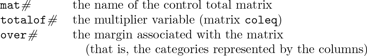
For the control total matrices #= 1, 2,…, the following meta information is stored.

mat #	the name of the control total matrix
totalof #	the multiplier variable (matrix coleq)
over #	the margin associated with the matrix (that is, the categories represented by the columns)

Also, ipfraking stores the notes regarding the control matrices used and which of the margins did not match the control totals, if any. See [D] notes.

The linear option provides linear calibration (case 1 of Deville and Särndal [1992]). The weights are calculated analytically:

$w_{j,\text{lin}}=w_{dj}(\text{1 }+x_j^{\prime }\lambda ),\hspace{0.17em}\lambda = {\left({\displaystyle \sum _{j\in \text{S}}{w}_{dj}{x}_j{x^{\prime }}_j}\right)}^{-1}\left\{T(X)-t(X)\right\}$

Because no iterative optimization is required, linear calibration works quickly. However, it undesirably may potentially produce negative weights because the range of weights is not controlled. Because raking works by multiplying the current weights by positive factors, if the input weights are all positive, the output weights will also be positive. Negative weights are not allowed by the official svy commands or commands that work with [pweight]. In many tasks, running linear weights first, pulling up the negative and small positive weights (replace weight = 1 if weight <= 1), and reraking using the “proper” iterative proportional fitting runs faster than raking from scratch. An example of linearly calibrated weights is given below in section 6.

2.3 Utility commands

The original package ipfraking provided additional utility commands: mat2do and xls2row. One of these utility commands, mat2do, was updated to provide the option notimestamp to omit the time stamps (which tend to unnecessarily throw off the project building and revision control systems).

This update provides two more utility commands, whatsdeff and totalmatrices.

Design effects

A new utility command, whatsdeff, was added to compute the unequal weighting (UWE) design effects (DEFFs) and margins of error. These are common tasks associated with describing survey weights. Specifically, the Transparency Initiative of the American Association for Public Opinion Research (AAPOR 2017) requires that

For probability samples, the estimates of sampling error will be reported, and the discussion will state whether or not the reported margins of sampling error or statistical analyses have been adjusted for the DEFF due to weighting, clustering, or other factors.

whatsdeff weight_variable [if] [in] [, by( varlist )]

The utility command whatsdeff calculates the apparent DEFF due to UWE,

${\text{DEFF}}_{\text{UWE}}=\text{ 1 }+{\text{CV}}_w^2=\text{1+r(Var)/(r(mean)})^2$

using the returned values from summarize weight_variable (see help return). Additionally, it reports the effective sample size, n/DEFF_UWE, and returns the margins of error for the sample proportions that estimate the population proportions of 10% and 50%.

DEFF can also be broken down by a categorical variable:

The estimates of UWE DEFFs that whatsdeff produces should be considered a typical magnitude of a DEFF. As pointed out by a referee, in many situations when survey variables are correlated with weights or with the variables that weight calibration is based on, the actual DEFFs reported by postestimation command estat effect should be expected to be lower, provided that variance estimation methods account for calibration properly, for example, via replicate variance estimation as described in Kolenikov (2010) or via the svy, vce(calibrate) functionality of the official Stata svy suite available in Stata 15.1+ (Valliant and Dever 2018). In other words, for most situations these estimates could be considered an upper bound on this DEFF because this calculation assumes that the weights are independent of the survey variable of descriptive interest.

Conversion of the matrices

A new command, totalmatrices, converts the control totals matrices between the formats expected by ipfraking and svycal (Valliant and Dever 2018).

totalmatrices matrix_list , stub( name ) [svycal ipfraking replace convert]

stub( name ) provides the naming convention for the converted control total matrices. If the conversion is from ipfraking to svycal, one matrix whose name is supplied in the stub() option will be created. If the conversion is from svycal to ipfraking, matrices corresponding to each variable will be created and have their names set to concatenation of the stub and the variable name. stub() is required.

svycal checks that the supplied matrix or matrices are compatible with svycal specification of totals as a matrix.

ipfraking checks that the supplied matrix or matrices are compatible with ipfraking. replace specifies that the matrices with the required names can be overwritten if they already exist in memory.

convert is used to request the conversion; otherwise, totalmatrices will check only that the format of the inputs seems to be correct.

If you want to convert several matrices from ipfraking format to a single matrix in svycal format, type

If you want to convert a single matrix compatible with svycal requirements for its totals( matrix_name ) format into a list of matrices compatible with ipfraking, type

Note that at the moment, totalmatricesdoes not handle conversion of interactions, which is arguably one of the greatest strengths of svycal. As noted in section 7, for interactions to work out with ipfraking, standalone variables need to be created, and totalmatrices would rather have the user do that.

2.4 New commands in the package

I added two new commands to the package, ipfraking_report and wgtcellcollapse, and I document them in the subsequent sections of this article. The former provides reports on the raked weights, including summaries of the unweighted data, data with the input weights, and data with the calibrated weights. The latter creates a mostly automated flow of collapsing weighting cells that are too detailed (and hence have low sample sizes).

3 Excel reports on raked weights: ipfraking_report

ipfraking_report using filename , raked_weight( weight_variable )

[matrices( matrix list ) by( varlist ) xls replace force]

The utility command ipfraking_report produces a detailed report describing the raked weights and places it into filename .dta (or, if the xls option is specified, both filename .dta and filename .xls).

Along the way, ipfraking_report runs a regression of the log raking adjustment ratio on the calibration variables. This regression is expected to have R ² equal to or close to 1 and residual variance equal to or close to 0. This naturally produces high t test values, but the purpose of this regression is not in establishing “significance” of any variable in explaining the outcome (which we know to be predicted with near certainty). Instead, the regression coefficients provide insights regarding which categories received greater versus smaller adjustments (which in turn indicate lower response or coverage rates for the corresponding population subgroups). Conversely, control variables that are associated with relatively similar adjustment factors may be contributing relatively little to the weight adjustment and may be candidates for removal from the list of control totals.

The regression output, using example 3 from Kolenikov (2014), is as follows:

We can see that ipfraking had to make greater adjustments to the weights of older females (sex_age==23, that is, sex==2 & age==3; the adjustment factor for this category was 3.732 versus the low of 1.798 for young women) and especially of individuals of other races (the adjustment factor was 9.023, versus 1.798 for the whites). The diagnostic value is in the differences in the adjustment factors with the same variable. Because no attempt is being made to average across the population or the sample or to assign the “base” variable, the absolute reported values of the adjustment factors may not be meaningful. In the example above, 1.798 figures both as the greatest adjustment factor of the region variable and as the lowest adjustment factor for the race and sex-by-age interaction. As is easily seen from regression output, this value is the exponent of the intercept 1.798=exp(0.586). Because all the “estimates” of the region-specific coefficients are negative, the lowest reported value is less than this baseline value. Because all the “estimates” of the race and sex-by-age indicators are positive, all the categoryspecific adjustment factors are greater than this baseline value. This is an interplay of the base categories and the differences in the demographic composition within each category of a control total variable vis-a-vis other weighting variables.

3.1 Options for ipfraking_report

raked_weight( weight_variable ) specifies the name of the raked weight variable to create the report for. raked_weight() is required.

matrices( matrix_list [matrix_list …] ) provides a list of known control totals. The ipfraking_report command will pick up the raking variables and their categories. Each matrix is expected to be compatible with the matrices consumed by ipfraking as control totals, the ctotal() option. While the functionality of producing results by different variables is provided with the by() option, passing the known control totals with matrices()allows comparing the required versus achieved control totals.

by( varlist ) specifies a list of additional variables for which the weights are to be tabulated in the raking weights report. The difference with the matrices() option is that the control totals for these variables may not be known (or may not be relevant). In particular, by(_one), where one is identically 1, will produce the overall report.

xls requests exporting the report to an Excel file.

replace specifies that the files produced by ipfraking_report (that is, the .dta and the .xls file if xls option is specified) should be overwritten.

force requests that ipfraking_report provide summaries of weights for a given variable each time it is encountered. The multiple opportunities include being one of the raking margins picked up from the control totals saved by ipfraking, meta; being supplied with the by() option; and being supplied with the matrices() option. The reasons to include a variable multiple times in these options is to see how the weights perform depending on whether a variable with known control totals is included as a raking margin.

3.2 Variables in the raking report

The raking report file contains the following variables.

Variable name	Definition
Weight_Variable	the name of the weight variable, generate()
C_Total_Margin_Variable _Name	the name of the control margin, rowname of the corresponding ctotal() matrix
C_Total_Margin_Variable _Label	the label of the control margin variable Variable_Class the role of the variable in the report: Raking margin: a variable used as a calibration margin (picked up automatically from the ctotal() matrix, provided the meta option was specified); Other known target: supplied with the matrices() option of ipfraking_report; Auxiliary variable: additional variable supplied with the by() option of ipfraking_report
C_Total_Arg_Variable _Name	the name of the multiplier variable
C_Total_Arg_Variable _Label	the label of the multiplier variable
C_Total_Margin_Category _Number	numeric value of the control total category
C_Total_Margin_Category _Label	label of the control total category
C_Total_Margin_Category _Cell	an indicator of whether a weighting cell was produced by collapsing categories using wgtcellcollapse
Category_Total_Target	the control total to be calibrated to (the specific entry in the ctotal() matrix)
Category_Total_Prop	control total proportion (the ratio of the specific entry in the ctotal() matrix to the matrix total)
Unweighted_Count	number of sample observations in the category
Unweighted_Prop	unweighted proportion
Unweighted_Prop_Discrep	difference Unweighted _Prop− Category _Total_Prop
Category_Total_SRCWGT	weighted category total with input weight
Category_Prop_SRCWGT	weighted category proportion with input weight
Category_Total_Discrep _SRCWGT	difference Category _Total_SRCWGT− Category_Total_Target
Category_Prop_Discrep_SRCWGT	difference Category _Prop_SRCWGT− Category_Total_Prop
Category_RelDiff_SRCWGT	reldif(Category_Total_SRCWGT, Category_Total_Target)
Overall_Total_SRCWGT	sum of source weights
Source	the name of the matrix from which the totals were obtained
Comment	placeholder for comments, to be entered during manual review

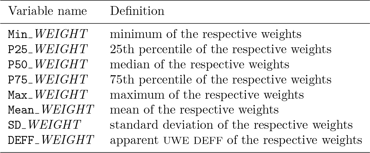
For each of the input weights (SRCWGT suffix), raked weights (RKDWGT suffix), and raking ratio (the ratio of raked and input weights, RKDRATIO suffix), the following summaries are provided.

Variable name	Definition
Min_WEIGHT	minimum of the respective weights
P25_WEIGHT	25th percentile of the respective weights
P50_WEIGHT	median of the respective weights
P75_WEIGHT	75th percentile of the respective weights
Max_WEIGHT	maximum of the respective weights
Mean_WEIGHT	mean of the respective weights
SD_WEIGHT	standard deviation of the respective weights
DEFF_WEIGHT	apparent UWE DEFF of the respective weights

3.3 Example

Continuing with the example of calibration by region, race, and sex-by-age interaction, we find that a glimpse of the raking report looks as follows:

The last line, corresponding to the auxiliary variable one identically equal to 1 (this variable was present in the dataset because it was used by ipfraking as a multiplier), contains summaries for the sample as a whole. I recommend to always include it (note the use of ipfraking_report,…by(_one) in the syntax in the previous section).

The functionality of ipfraking_report is aimed at manual quality control, which typically involves i) review of variables and categories with raking factors that differ the most (in the output such as that shown on page 152) and ii) review of the resulting report file in Excel (for example, for DEFFs and discrepancies between targets and achieved totals).

4 Collapsing weighting cells: wgtcellcollapse

An additional new component of the ipfraking package is a tool to semiautomatically collapse weighting cells to achieve a required minimal size of the weighting cell. A typical recommendation is to have cells of size at least 30 to 50.

wgtcellcollapse task [if] [in] [, task_options]

where task is one of the following:

report lists the currently defined collapsing rules.

define defines collapsing rules explicitly.

sequence creates collapsing rules for a sequence of categories.

candidate finds rules applicable to a given category.

label labels collapsed cells using the original labels after wgtcellcollapse collapse. collapse performs cell collapsing.

4.1 wgtcellcollapse report

Syntax

wgtcellcollapse report, variables( varlist ) [break]

Options

variables( varlist ) specifies the list of variables for which to report the collapsing rules. variables() is required.

break makes wgtcellcollapse report exit with an error when technical inconsistencies are encountered.

4.2 wgtcellcollapse define

Syntax

wgtcellcollapse define, variables( varlist ) [from( numlist ) to( # ) label( string ) max( # ) clear]

Options

variables( varlist ) specifies the list of variables for which the collapsing rule can be used. variables() is required.

from( numlist ) specifies the list of categories that can be collapsed according to this rule.

to( # ) specifies the numeric value of the new collapsed category.

label( string ) provides the value label to be attached to the new collapsed category.

max( # ) overrides the automatically determined max value of the collapsed variable.

clear clears all the rules currently defined.

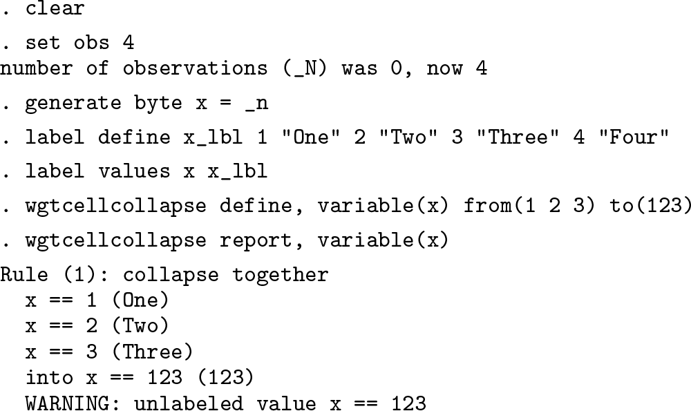
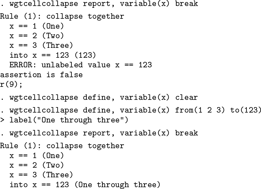
Example

Let us demonstrate the two subcommands introduced so far with the following toy example.

For automated quality control purposes, the break option of wgtcellcollapse report can be used to abort the execution when encountering technical deficiencies in the rules or in the data. In the above example, the label of the new category 123 was not defined. Should the break option be specified, an absence of the category label would be considered a serious enough deficiency to stop with an error:

4.3 wgtcellcollapse sequence

Syntax

wgtcellcollapse sequence, variables( varlist ) from( numlist ) depth( # )

Options

variables( varlist ) specifies the list of variables for which the collapsing rule can be used. variables() is required.

from( numlist ) specifies the sequence of values from which the plausible subsequences can be constructed. from() is required.

depth( # ) specifies the maximum number of the original categories that can be collapsed. depth() is required.

Example

Continuing with the toy example introduced above, let us see an example of moderatelength sequences to collapse categories:

Note how wgtcellcollapse sequenceautomatically created labels for the collapsed cells.

When creating sequential collapses, wgtcellcollapse sequence uses the following conventions in assigning the values for the new collapsed categories:

First comes the length of the collapsed subsequence (up to depth( # )).

Then comes the starting value of the category in the subsequence (padded by zeros as needed).

Then comes the ending value of the category in the subsequence (padded by zeros as needed).

In the example above, rules 7 through 9 lead to collapsing into the new category 324, which stands for “the subsequence of length 3 that starts with category 2 and ends with category 4”. A numeric value of the collapsed category that reads like 50412 means “the subsequence of length 5 that starts with category 4 and ends with category 12”. In that second example, wgtcellcollapse sequence padded the value of 4 with an additional 0, so the length of resulting collapsed category value is always (number of digits of the sequence length) +twice (number of digits of the greatest source category).

Note that wgtcellcollapse sequence respects the order in which the categories are supplied in the from() option and does not sort them. If the categories are supplied in the order 2, 4, 1, and 3, then wgtcellcollapse sequence would collapse 2 with 4, 4 with 1, and 1 with 3:

4.4 wgtcellcollapse candidate

Syntax

wgtcellcollapse candidate, variable( varname ) category( # ) [maxcategory( # )]

Options

variable( varname ) specifies the variable to be collapsed. variable() is required.

category( # ) specifies the category to be collapsed. category() is required.

maxcategory( # ) specifies the maximum value of the categories in the candidate rules to be returned.

Example

The rules found are quietly returned through the mechanism of sreturn (see [P] return) because they are intended to stay in memory sufficiently long for wgtcellcollapse collapse to evaluate each rule. Going back to the example from the previous section with sequential collapses of depth 3, we can identify the following candidates for categories 2 and 212 (collapsed values of 1 and 2) and a nonexistent category of 55:

In the second call to the option, we used max(9) to restrict the returned rules to the rules that deal only with the original categories (so rule 8 that involved a collapsed category 234 was omitted). It relies on the naming conventions described in the previous section: any of the collapsed cells would have three-digit values. In the third call, we requested a list of rules that involve a collapsed category cat(212). Requests for nonexisting categories are not considered errors but simply produce empty lists of “good rules”.

4.5 wgtcellcollapse label

Syntax

wgtcellcollapse label, variable( varname ) [ verbose force]

Options

variable( varname ) specifies the collapsed variable to be labeled. variable() is required.

verbose outputs the labeling results. There may be a lot of output.

force instructs wgtcellcollapse label to use only categories present in the data.

Example

An example is given in section 5.2 below.

4.6 wgtcellcollapse collapse

Syntax

wgtcellcollapse collapse [ if] [in] , variables( varlist ) mincellsize( # ) saving( dofile_name ) [generate( newvar ) replace append feed( varname ) strict sort( varlist ) run maxpass( # ) maxcategory( # ) zeroes( numlist ) greedy]

Options

variables( varlist ) provides the list of variables whose cells are to be collapsed. When more than one variable is specified, wgtcellcollapse collapseproceeds from right to left, that is, first attempts to collapse the rightmost variable. variables() is required.

mincellsize( # ) specifies the minimum cell size for the collapsed cells. For most weighting purposes, values of 30 to 50 can be recommended. mincellsize() is required.

saving( dofile_name )specifies the name of the do-file that will contain the cell-collapsing code. saving() is required.

generate( newvar ) specifies the name of the collapsed variable to be created.

replace overwrites the do-file if one exists.

append appends the code to the existing do-file.

feed( varname ) provides the name of an already existing collapsed variable.

strict modifies the behavior of wgtcellcollapse collapse to use only collapsing rules for which all participating categories have nonzero counts.

sort( varlist ) sorts the dataset before proceeding to collapse the cell. The default sort order is in terms of the values of the collapsed variable. A different sort order may produce a different set of collapsed cells when cells are tied on size.

run specifies that the do-file created is run upon completion. This option is typically specified with most runs.

maxpass( # ) specifies the maximum number of passes through the dataset. The default is maxpass(10000).

maxcategory( # ) specifies the maximum category value of the variable being collapsed. It is passed to the internal calls to wgtcellcollapse candidate; see above.

zeroes( numlist )provides a list of the categories of the collapsed variable that may have zero counts in the data.

greedy modifies the behavior of wgtcellcollapse collapse to prefer the rules that collapse the maximum number of categories.

Remarks

The primary intent of wgtcellcollapse collapse is to create the code that can be used in both a survey data file and a population targets data file that are assumed to have identically named variables. Thus, it not only manipulates the data in memory and collapses the cells but also produces the do-file code that can be recycled in automated weight production. To that effect, when a do-file is created with the replace and saving() options, the user must specify the generate() option to provide the name of the collapsed variable; and when the said do-file is appended with the append and saving() options, the name of that variable is provided with the feed() option.

The algorithm wgtcellcollapse collapse uses to identify the cells to be collapsed uses a variation of greedy search. It first identifies the cells with the lowest (positive) counts; finds the candidate rules for the variable or variables to be collapsed; evaluates the counts of the collapsed cells across all of these candidate rules; and uses the rule that produces the smallest size of the collapsed cell across all applicable rules. So when it finds several rules that are applicable to the cell being currently processed that has a size of 5, and the candidate rules produce cells of sizes 7, 10, and 15, wgtcellcollapse collapse will use the rule that produces the cell of size 7. The algorithm runs until all cells have sizes of at least mincellsize( # ) or until maxpass( # ) passes through the data are executed. In real-world situations with messy data, this basic algorithm often produces inconsistent results generally because it fails to identify empty cells or fully track the cells that have already been collapsed. For that reason, I provide some hints to modify its behavior. Section 5 demonstrates a worked-out example.

Hint 1. Because wgtcellcollapse collapse works with the sample data, it will not be able to identify categories that are not observed in the sample (for example, rare categories missing because of unit nonresponse) but may be present in the population. This will lead to errors at the raking stage, when the control total matrices have more categories than the data, forcing ipfraking to stop with errors. (See page 147 for the output ipfraking provides in this situation.) To help with that, the option zeroes() allows the user to pass the categories of the variables that are known to exist in the population but not in the sample.

Hint 2. The behavior of wgtcellcollapse collapse, zeroes() leads to undesirable artifacts when collapsing long streaks of sequential zeros. While the edge zero cells would be collapsed with their nonzero neighbors, the zero cell in between may end up being collapsed with some faraway cells, creating collapsing rules with breaks in the sequences. To improve upon that behavior, the option greedy makes wgtcellcollapse collapse look for a rule that combines as many cells as possible, thus collapsing as many categories with zero counts in one pass as it can.

Hint 3. Other than for dealing with zero cells, the option strict should be specified most of the time. It ensures that each cell in a candidate rule being evaluated has some data in it.

Hint 4. If you want to guarantee some specific combination of cells to be collapsed by wgtcellcollapse collapse, the most reliable way is to explicitly identify them with the if qualifier and specify a very large cell size like mincellsize(10000) so that wgtcellcollapse collapse makes every possible effort to collapse those cells. Because the resulting cell or cells will fall short of that size, the program will exit with a complaint that this size could not be achieved, but hopefully the cells will be collapsed as needed.

Hint 5. If any of the cells fail to reach the required sizes, the problematic values are returned to the user in the r(failed) macro as a space-delimited list and in the r(cfailed) as a comma-delimited list. The content of the r(failed) macro can be used in code that could read

while the content of the r(cfailed) macro can be used in code that could read

list…if inlist( collapsed_variable ,`r(cfailed)´)

Also, these returned values should be used in production code by using the assert command (Gould 2003) to ascertain that these macros are empty (that is, no errors were encountered):

assert "`r(failed)´" == ""

A referee noted that wgtcellcollapse could also have utility in preparing for hotdeck imputation procedures. The textbook versions of hotdeck procedures impute missing data by assuming a missing at random model (Rubin 1976) with conditioning on a set of categorical variables, that is, cells of a multivariate table. Akin to weighting procedures, hotdeck procedures are more stable with larger cells, so cell collapsing is often recommended to achieve minimal cell sizes (with an understanding of the bias-versusvariance tradeoff built into these collapsing decisions). For a review of the hotdeck and related imputation methods, see Andridge and Little (2010).

5 Extended motivating example

The primary purpose of developing wgtcellcollapse and adding it to the ipfraking suite was to address the need to collapse cells of the margin variables so that each cell has a minimum sample size in a way that can be easily made consistent between a sample data and the population targets data. The problem arises when some of the target variables have dozens of categories, most of which have small counts. Example where such needs arise include

transportation surveys, where many stations will have low counts of boardings, alightings, or both;

country of origin variables in household surveys, where most countries will have very low counts; and

continuous age variables that can be collapsed into age groups differently for different values of race or sex.

The workflow of wgtcellcollapse is demonstrated with the following simulated transportation dataset of trips along a commuter metro line composed of 21 stations:

Suppose turnstile counts were collected at entrances (board_id) and exits (alight_id) of these stations, producing the following population figures:

Most people ride the train to the last station, with much smaller traffic at other population centers.

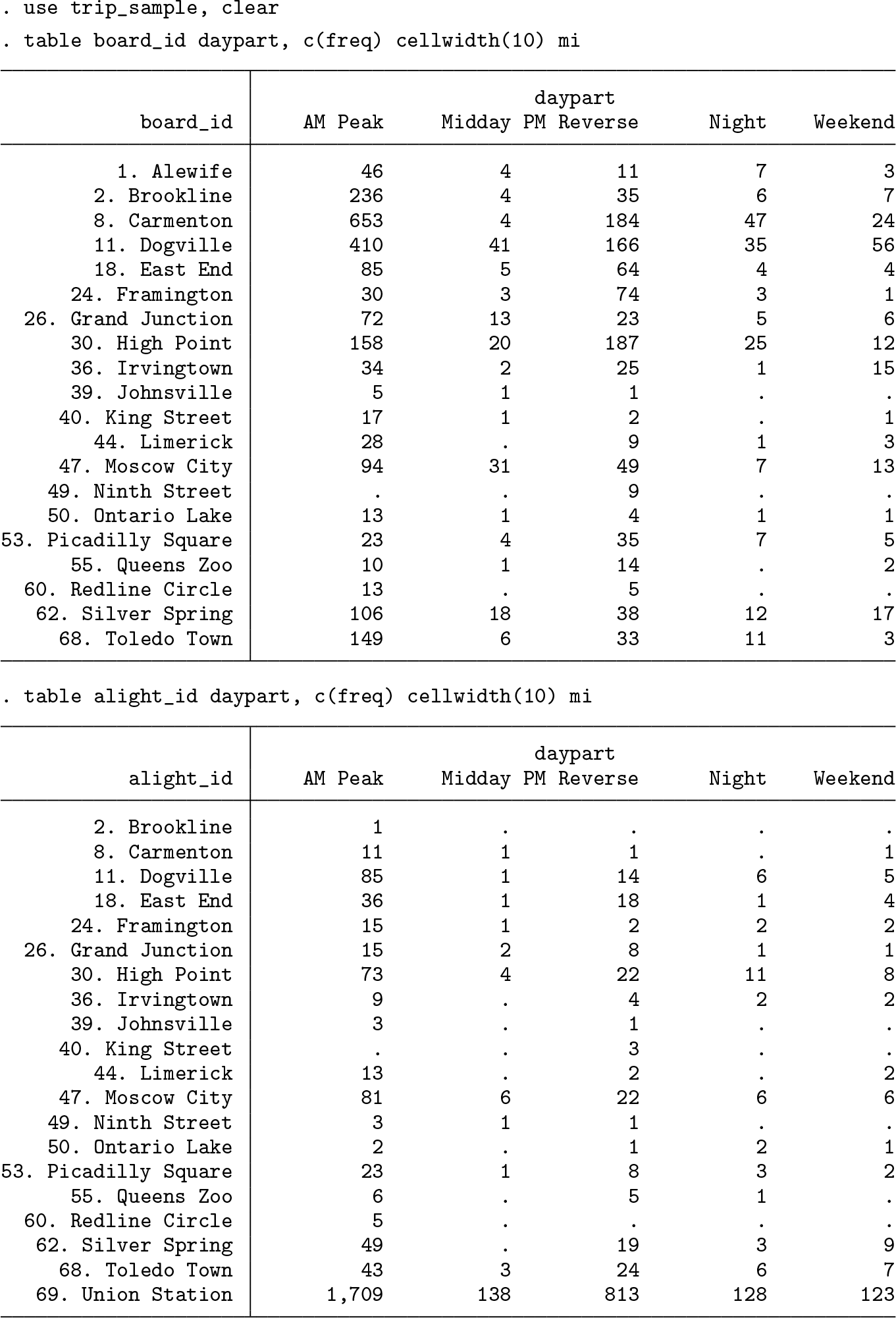
Suppose a survey was administered to a sample of the metro line users, with the following counts of cases collected.

Because only 3,654 surveys were collected from a total of 96,783 riders, we would reasonably expect that there is a need for weighting and nonresponse adjustment. The data available for calibration include the population turnstile counts listed above. We will produce interactions of the day part and the station that will serve as two weighting margins (one for the stations where the metro users boarded and one for the stations where they got off).

First, we need to define the weighting rules. In this case, the stations are numbered sequentially, with the northernmost station Alewife being number 1 and the southernmost station, Union Station, where everybody gets off to rush to their city jobs or attractions, being number 69. Below, we create a list of stations and provide it to wgtcellcollapse sequence. We would be collapsing stations along the line with the expectation that travelers boarding or leaving at adjacent stations within the same day part are more similar to one another than the travelers boarding or leaving a particular station at different times of the day. Collapsing rules need to be defined for the daypart variable as well—mostly because wgtcellcollapse collapse expects all variables to have collapsing rules defined.

The syntax above relies on the stations being in the sequential order, which is how the output of levelsof is organized. Otherwise, the internal numeric identifiers of the stations would need to be supplied in the order in which the trains run through them.

The number of collapsing rules for variables board_id and alight_id created by wgtcellcollapse sequence is 2,961 each.

Below, we present the final syntax to produce the collapsed cells. A more detailed version of this article, available upon request from the author, describes the process of building the syntax through trial and (mostly) error. A reader who plans to thoroughly use wgtcellcollapse should read the full description.

Each pass identified the smallest cell count, the cell where this low count is found, the rule that can be used to collapse this cell with some other cell (see more on determination of what wgtcellcollapse believes to be the best rule below), and Stata code that can be used to apply this collapsing rule.

The collapsed values of dpston (daypart-station-on) and dpstoff (daypart-stationoff) combine the values of the parent variables. The value of dpston==1000003 indicates the combination of categories daypart==1 and station number 3. The value of dpston==1023940 indicates daypart==1 and sequence of two stations from 39 to 40. The value of dpston==2053044 indicates daypart==2 and sequence of five stations from 30 to 44.

The first call to wgtcellcollapse uses the options generate() and replace to create a new variable and a new do-file, while subsequent calls feed() this variable back and append additional cell-collapsing code to the existing do-file.

The zeroes() option specified in calls 1, 3, and 4 notified wgtcellcollapse that there are values of alight_id that are never observed. (Riders get on the train on these stations and exit in small numbers, but no completed surveys were obtained.) The mincellsize(1) option effectively instructed wgtcellcollapse to exit once all of these zero cells are identified and merged with nonzero cells. The maxcategory(99) option restricts collapsing rules only to those that involve individual stations. It relies on the convention that all the individual station IDs are less than 99 and all the collapsed values are at least 20102 (that is, the first two stations merged together, forming a cell of size 2 that stretched from 01 to 02). Without these options, wgtcellcollapse would be allowed to pick up one of the previously collapsed cells. However, it seems safer to collapse stations with zero count to only one station.

Using the subsampling conditions like if daypart==5 & inrange(alight_id,1,36) in calls 5 and 6 effectively specifies one specific collapsing cell that the algorithm could not otherwise identify. A higher target value, mincellsize(50), is used in conjunction to ensure that the algorithm does not exit prematurely. The special missing value .i that appears in the smallest count report, as opposed to the actual counts in other runs, is used internally to stop wgtcellcollapse after all the relevant cases selected by the if qualifier have been processed.

Using the greedy option in call 3 made it possible to collapse the streak of zero counts in the midday part from 36. Irvington to 44. Limerick. Without it, each individual zero count station would be paired with a nonmissing station, which leads to cells that overlap in space.

After all zero counts stations are processed, the strict option should almost always be specified, as is done in runs 2, 5, 6, and 7. It prevents wgtcellcollapse from picking up rules that may have skipped categories in them. In other words, it ensures that the collapsed cells are contiguous.

The resulting cells satisfy the sample size requirements of at least 20 cases per cell:

. by dpston5, sort: assert _N >= 20

by dpstoff5, sort: assert _N >= 20

5.1 Pipeline to raking

As its output, wgtcellcollapse produced two files, one for each weighting margin, called dpston.do and dpstoff.do. An interested reader is welcome to type them; they contain long sequences of replace commands to perform the cell collapsing. These do-files are intended to be run on both the sample and the population data to create identical collapsed categories and produce consistent matrices of the population control totals for ipfraking.

5.2 Informative labels

Once the collapsing rules are finalized, several types of category labels can be attached to the resulting collapsed cells. Using the mechanics of labels in multiple languages (see [D] label language), wgtcellcollapse label defines three “languages” to describe the cells. The language numbered_ccells may be convenient for debugging purposes in fine-tuning the collapsing algorithms, while the language texted_ccells would prove useful for ipfraking_report in creating human-readable labels. In Stata Markup and Control Language output, the label language instructions are clickable, so the user can click the command rather than copying and pasting it.

6 Linear calibrated weights

Using the final set of collapsed categories in the simulated transportation data example, let us demonstrate the linear calibration option of ipfraking, added since Kolenikov (2014). In mathematical terms, linear weights explicitly solve the minimization problem of finding a set of weights $\left\{w_{li}, i=\text{ 1}, . . . , n\right\}$ , where the subscript l stands for linear calibration, such that

${\displaystyle \sum _{ i=1}^n\frac{{(w_{li}-w_{di})}^2}{w_{di}}}\to \text{min}$

Deville and Särndal (1992) and Särndal, Swensson, and Wretman (1992) provide explicit treatment of the problem and the resulting analytical expressions that are coded in ipfraking, linear. The main advantage of linear weight calibration is a much faster computing time. To demonstrate it, we will time the output by using the immediate timing results, set rmsg on (see [R] set).

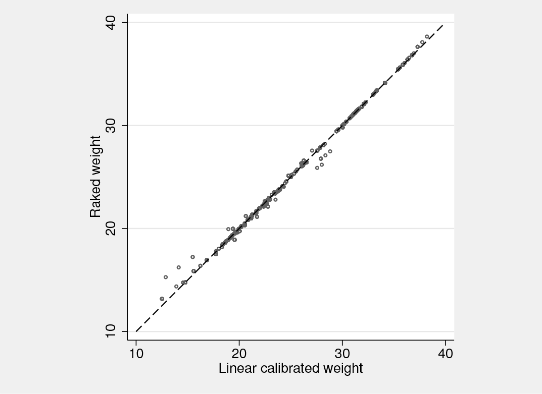
The speed advantages of linear calibration are quite clear (0.43 seconds versus 0.99 seconds), although raking convergence in 8 iterations is quite fast in my experience. It is not unusual to see dozens of iterations, and when higher order interactions are being used as raking margins, subtle correlations between the cells arise, slowing down convergence and requiring hundreds of iterations. Linear calibrated and raked weights are similar, as figure 1 demonstrates. However, the lowest of the linearly calibrated weights are slightly smaller than comparable raked weights. The weights produced by linear and raking calibration methods should be expected to agree in general, but the match along the diagonal line of the plot should not be expected to be ideal.

Figure 1.

Linear and raked weights

As mentioned before, in extreme situations, linearly calibrated weights may become negative, which creates additional issues. First, Stata’s svy commands or estimation commands with pweight specifications do not accept negative weights and produce error messages when such weights are encountered. This is not a bug but indeed a welcome behavior. Second, negative weights are typically difficult to interpret; within a common, although not technically accurate interpretation of sampling weights as the number of population units that a sampled unit represents, it is puzzling to find a negative number of such population units. The way I use the linear calibration functionality of ipfraking is to produce “preliminary” sets of weights. If the weights at the low end satisfy the natural range restriction (greater than 0, to prevent input data check errors with estimation commands; or in some applications, greater than 1, to satisfy the “number of population units” interpretation that is often desirable), these weights can be “accepted” as final. If they do not, ipfraking can be called with trimming syntax such as trimloabs(1). The linear weights can then be used as a starting point to accelerate convergence using the from() option.

While the general theory of calibrated estimation (Deville and Särndal 1992) ensures that linear calibrated weights (analyzed as case 1 in that article) and raked weights (case 2) are asymptotically equivalent, this equivalence implicitly requires that the scales of the population control matrices are identical. In practice, different control total variables may come from different sources, and some sources may either have different populations to which they can technically be generalized or come at different scales such as proportions versus population totals. Nearly every dual-frame random-digit dialing survey of the general U.S. population that I dealt with would use the American Community Survey data for demographic variables (which would come with the desirable population scaling) and National Health Interview Survey data for phone use variables (cell phone only, landline only, both, or none), which would come in the form of proportions. While the raking version of ipfraking would not have any difficulty incorporating both (with the caveat that the final scale of weights will be determined by the last variable in the ctotal() list), the linear version of weights would try to find a middle point between the population totals that are on the scale of millions and proportions that are on the scale of about 1. The results would likely be quite strange.

7 Other packages with similar functionality

Other packages provide similar basic functionality (that is, raked weights, with or without trimming). Kolenikov (2014) provided comparisons with survwgt (Winter 2002), ipfweight (Bergmann 2011) and maxentropy (Wittenberg 2010) and reported that the weights produced by these packages were identical within numeric accuracy.

Concurrently with Kolenikov (2014), another weight calibration package, sreweight (Pacifico 2014), was published in the Stata Journal. It implements a full range of objective functions from Deville and Särndal (1992) and does so faster than ipfraking because the core iterative functionality is implemented in Mata. Finally, Stata 15.1 now provides the svycal command, undocumented at the time of the writing of this article, although described and exemplified in detail in Valliant and Dever (2018). Compared with svycal, the core functionality of ipfraking provides a richer set of trimming specifications. I compared the weights produced by ipfraking with those produced by sreweight and svycal in the case of the basic raking procedure without trimming, and they agree within numeric accuracy:

Weights produced by ipfraking also agree with those produced by the R package survey( Lumley 2010, 2018), namely, the survey::calibrate(…,calfun="raking") function, and those produced by SAS raking macro RAKE_AND_TRIM()(Izrael et al. 2017). When trimming options are specified, the results from different packages diverge because trimming operations appear to be implemented differently in each package.

It is unfortunate that so much effort has gone into replicating the functionality by the different authors. The primary distinction of the current ipfraking package is the rich ecosystem that goes along with it, aimed at producing survey weights by a survey organization in a way that is efficient, robust, and flexible codewise.

As a practicing survey statistician who needs to experiment with the weights a lot, I believe that ipfraking is easier to experiment with than svycal or sreweight for several reasons. First, ipfraking relies on the control totals being carried over from svy: total with minimal modifications such as renaming row and column names; passing control totals is more cumbersome with other packages. Second, ipfraking produces detailed diagnostics of problems and oddities it encounters along the way, assisting the survey statistician in assessing whether the resulting weights are satisfactory.

For relatively simpler tasks of producing replicate weights and calibrating them at the same time, survwgt provides easier syntax. Coding the task with ipfraking or any other package would require explicit cycles.

From a code development perspective, I believe that relying on matching the order of control totals and variables, as required by all other community-contributed packages, creates a potential for errors that are easy to make and difficult to catch. If you supplied 20 control totals and 19 variables, at which position in the list should the 20th missing variable be? With ipfraking and the official svycal, the risk that a control total figure would be associated with a wrong category of the control total variable is much lower because they pair the values and the categories in a single object (via the names attached to the control total matrices) or explicit syntax value.variable = # specification of svycal. However, the matrix naming is different between ipfraking and svycal, so I provide a conversion tool, totalmatrices, in this update.

Additionally, ipfraking can incorporate variables that sum up to different totals, for example, totals from different sources or years, or totals and proportions if unified data are not available, with the side effect of producing weights whose totals agree with the last control total variable. Without trimming, doing so ensures that proportions for each calibration variable are satisfied. Because maxentropy, sreweight, and svycal produce weights by optimization with the goal of satisfying all totals simultaneously, it is unclear what the properties of the resulting weight would be when the scales of control totals differ between variables and whether the resulting weights would produce marginal proportions that agree between the control totals and calibrated weights.

Compared with ipfraking, the official svycal command handles interactions far more graciously and consistently with the Stata user experience of using factor variables in regression models (see [U] 11.4.3 Factor variables). It creates the necessary interactions internally on the fly, while ipfraking requires explicit generation of interaction variables.

Finally, of all the Stata weight calibration packages, ipfraking is unique in offering the possibility of using multipliers other than 0 and 1 (that is, category dummies).

Ultimately, the choice of the package is a matter of personal preference, package familiarity, and coding style.

Supplemental Material

Supplemental Material, st0323_1 - Updates to the ipfraking ecosystem

Supplemental Material, st0323_1 for Updates to the ipfraking ecosystem by Stanislav Kolenikov in The Stata Journal