
Abstract
Spatial microsimulation encompasses a range of alternative methodological approaches for the small area estimation (SAE) of target population parameters from sample survey data down to target small areas in contexts where such data are desired but not otherwise available. Although widely used, an enduring limitation of spatial microsimulation SAE approaches is their current inability to deliver reliable measures of uncertainty—and hence confidence intervals—around the small area estimates produced. In this article, we overcome this key limitation via the development of a measure of uncertainty that takes into account both variance and bias, that is, the mean squared error. This new approach is evaluated via a simulation study and demonstrated in a practical application using European Union Statistics on Income and Living Conditions data to explore income levels across Italian municipalities. Evaluations show that the approach proposed delivers accurate estimates of uncertainty and is robust to nonnormal distributions. The approach provides a significant development to widely used spatial microsimulation SAE techniques.
Large-scale surveys are designed to obtain reliable estimates at national level or, in some instances, for large subnational scales such as regions. These can be considered to be the planned domains of the survey sampling design (Benavent and Morales 2016). However, there is a growing demand from both research and policy communities for various local estimates at more detailed spatial resolutions such as municipalities or neighborhoods due to the absence of data at such small area scales from existing census or administrative sources. However, this small area desire frequently encounters a problem of unplanned domains, given that for cost reasons such small areas typically have small or zero sample sizes in the survey sampling design. In these circumstances, commonly used direct estimators such as the Horvitz–Thompson estimator (Horvitz and Thompson 1952) that only use sample survey information either cannot be used (in the case of zero sample size domains) or provide unacceptably large variability in the estimates to be practically useful (in the case of small sample size domains).
In such scenarios, indirect small area estimation (SAE) of target population parameters has become a relatively widely used and increasingly demanded methodological technique via a range of SAE approaches. We refer to Rao and Molina (2015), Whitworth (2013), Rahman and Hardin (2017), and Marshall (2010) for useful methodological reviews on both regression-based and microsimulation-based SAE methods. Spatial microsimulation approaches, sometimes referred to as survey calibration approaches (Espuny-Pujol, Morrissey, and Williamson 2018), represent a family of reweighting approaches to SAE in which the challenge is to reweight the survey units such that they optimally fit the demographic and socioeconomic profile of each small area according to a selected set of benchmark constraints. Part of the appeal of spatial microsimulation approaches to SAE for both researchers and policy users is their intuitive and accessible appeal without much of the complex statistical expertise required within many regression-based SAE methods, particularly as assumptions fail or more complex outcomes are desired. In those circumstances, one advantage of spatial microsimulation approaches over regression-based SAE estimators is that they tend to be more robust to failures in model assumptions, given that as model-assisted estimators it is only necessary that the population be reasonably well described by an assumed model for that model to be valid (Särndal, Swensson, and Wretman 1992).
Spatial microsimulation SAE approaches have been used to produce small area estimates across a range of policy areas including child malnutrition (Johnson et al. 2012), obesity (Edwards et al. 2010), fuel poverty (Office for National Statistics 2019), income and poverty (Bell, Basel, and Maples 2016; Pratesi 2016; World Bank 2018), regional planning (Clarke and Holm 1987), participation in sport (Ipsos MORI 2018), and transport (Lovelace, 2016; Ravulaparthy and Goulias 2011; Tribby and Zandbergen 2012). Spatial microsimulation SAE approaches have been well validated against known external data and against alternative regression-based SAE techniques (Moretti and Whitworth 2019; Tanton, Williamson, and Harding 2014; Whitworth and Carter 2015). Spatial microsimulation SAE has also been used effectively to assess the spatial impacts of differing “what if” policy scenarios (Chin and Harding 2006; Cullinan, Hynes, and O’Donoghue 2006; Tanton and Edwards 2013; Williamson, Birkin, and Rees 1998). For example, Campbell and Ballas (2013) introduce the SimAlba spatial microsimulation model Scotland in order to estimate the simulated impact of various policy scenarios on individual’s health outcomes. In an Australian context, Tanton and Edwards (2013) use spatial microsimulation SAE to assess the geographical impacts on expected elderly poverty levels from changes to the state pension (Tanton et al. 2009).
However, despite these widespread applications and contributions, an important long-standing limitation of spatial microsimulation SAE approaches is their continued inability to deliver estimates of uncertainty around central point estimates at small area level. More specifically, one faces something of a trade-off with any SAE approach in seeking via the indirect SAE estimates to reduce variance compared to the direct estimates while acknowledging that those direct estimates are unbiased compared to the indirect SAE estimates that are inherently biased. As such, it is essential when calculating the uncertainty of any SAE estimator that the mean squared error (MSE) is used, given that this takes into account both variance and bias. However, calculating MSE is often challenging in an SAE content and particularly so in spatial microsimulation approaches. In the case of design-based estimators, the design weights are known before the sample selection and are therefore nonrandom meaning that analytical approximations of MSE are available (Särndal et al. 1992). However, this is no longer the case in spatial microsimulation approaches to SAE when reweighing algorithms are used as the weights become random variables themselves. In these scenarios, analytical approximation of MSE becomes highly challenging, given that bias and variance cannot be computed in closed form such that empirically based resampling techniques are instead required to estimate their uncertainty (Chen and Shen 2015). Some analytical approximations have been suggested in the literature (D’Arrigo and Skinner 2010; Deville and Särndal 1992), but Chen and Shen (2015) highlight important practical challenges around the requirement for joint selection probabilities that are rarely computed or known in practice.
Empirical attempts to estimate the uncertainty around spatial microsimulation SAE estimates have been proposed in recent years (Chen and Shen 2015; Nagle et al. 2014; Whitworth et al. 2017), though none entirely successful. In response, this article develops a novel modified parametric bootstrap technique in order to estimate the uncertainty of spatial microsimulation small area estimates based on the MSE such that it captures both bias and variance components in the uncertainty estimate, unlike previous attempts. Our approach benefits from clear statistical properties under a linear model and can be used flexibly across alternative spatial microsimulation SAE techniques.
The remainder of this article is structured as follows. In the second section, the general problem of SAE of the population mean using iterative proportional fitting (IPF) is outlined. In the third section, the challenge of uncertainty estimation in SAE contexts is further described, and our approach to MSE estimation via bootstrap is detailed. In the fourth section, the bootstrap approach is evaluated via a simulation study, and in the fifth section, a practical data application focusing on Italian Statistics on Income and Living Conditions (SILC) data is presented to illustrate the approach. The sixth section provides a concluding discussion focusing on wider implications for spatial microsimulation SAE and potential next steps for research.
SAE With IPF
This section sets out the SAE problem of the population mean and formally introducing the IPF spatial microsimulation approach used in the later development of our proposed uncertainty estimator.
The General SAE Problem for a Small Area Mean
Let us consider a sample
Due to the unplanned domain problem, nd
may be too small (even zero) for many small areas in the survey data to compute reliable direct estimates of
Reweighing Using the IPF Algorithm
IPF is one of three main spatial microsimulation approaches to SAE—IPF, generalized regression reweighting and combinatorial optimization. To demonstrate our approach to the estimation of uncertainty in spatial microsimulation SAE, we focus on the IPF algorithm, given that this is both widely used and a constructively challenging test of our MSE estimator, given that its iterative nature renders the survey weights random variables themselves (Chen and Shen 2015; Rahman et al. 2013; Simpson and Tranmer 2005).
Like all spatial microsimulation SAE approaches, IPF can be understood as a reweighting optimization problem where the aim is to reweight the survey units (e.g., individuals or households) such that they optimally fit the demographic and socioeconomic profile of each small area according to a selected set of benchmark constraints (e.g., age-sex, employment status, ethnicity, health, education). Deville and Särndal (1992) provide a statistical theory of these reweighting techniques and alternative approaches. For each local area, the result is a tailored set of reweighted survey cases that fit to the benchmark characteristics of that small area in terms both of total population and the profile of that population across the benchmark constraints. A key data set created during IPF is a weights matrix giving new weights for each survey unit in each separate small area. For each small area, those final IPF weights show how representative each survey unit is of each area given their respective characteristics across the benchmarks. Across all survey individuals, these reweighted units sum to the small area population total and map onto its population profile across the benchmarks. As such, these reweighted data provide a valuable synthetic micropopulation for each small area that can be employed in further local analyses (e.g., “what if” policy simulations) as desired (Anderson 2013; Lovelace and Dumont 2016).
Formally, IPF can be understood as follows. Let wi
be the initial weight (usually the survey design weight) for
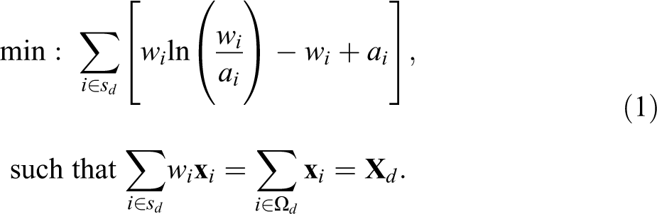
As noted above, (1) unfortunately does not have a closed-form solution such that solution via analytical approximation is required. This is however highly challenging. The IPF algorithm is therefore employed iteratively across the benchmark constraints in order to estimate the final weights for each survey unit in order to derive a solution empirically. To describe the IPF method more fully, the terminology and notation used by Kolenikov (2014) is followed: Initialize the iteration counter Increment the iteration counter Update the weights through each of the benchmark constraint variables in turn, If the discrepancies between The weights
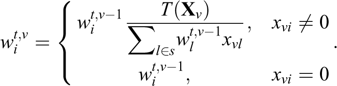
The benchmark constraints used for the survey reweighting are usually categorical variables in real applications. Therefore,

where
The IPF estimator can therefore be defined as follows:
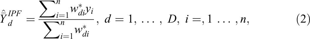
where
Measuring the Uncertainty: the MSE Estimator of
The quality of an estimate is assessed with reference both to its accuracy (bias) and to its precision (variability). It is therefore important to capture both aspects in any measure of uncertainty (Dodge and Commenges 2006; Statistics Canada 2009). The bias of an estimate can be defined as its degree to which it describes the measured phenomena correctly, in other words its difference from the true (though often unobserved) population value. In contrast, the variability of an estimate relates to how closely repeated observations confirm themselves (e.g., under random sampling). Figure 1 reproduces a visual summary of these two considerations from Ferrante and Cameriere (2009).
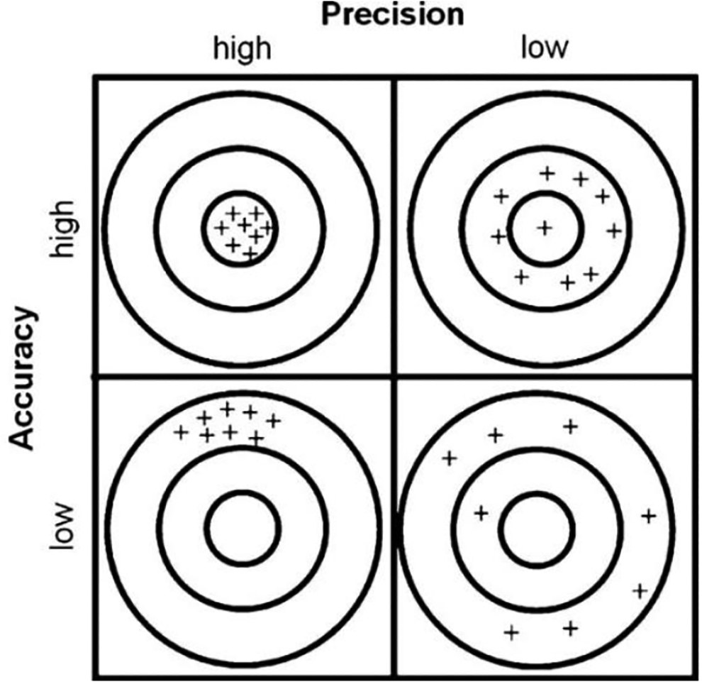
Precision and accuracy in estimates.
The MSE is the second moment about the origin of the error and thus takes into account both bias and variance. It is therefore an appropriate measure for our proposed estimation of uncertainty around spatial microsimulation SAE estimator. For the design unbiased direct survey estimates, the MSE is equal to the variance, while for the indirect SAE estimator, the MSE is equal to the bias squared plus the variance. As such, the attractiveness of any indirect SAE estimator compared to the unbiased direct estimator is dependent upon the reductions in variance in any SAE approach exceeding its increases to bias such that the MSE of the indirect SAE estimator is smaller than the MSE of the direct estimator. This is possible in SAE contexts where small areas have low or no survey sample sizes such that direct small area estimates are either nonviable or come with large variance.
Capturing the MSE via resampling techniques such as the bootstrap is common within regression-based SAE approaches (González-Manteiga et al. 2008b; Marchetti et al. 2018; Moretti, Shlomo, and Sakshaug 2018). Indeed, González-Manteiga et al. (2008b) point out that even when analytical approximations are available, bootstrap resampling might provide more accurate estimates due to its second-order accuracy, a property discussed further in Efron and Tibshirani (1993). However, no similar MSE measures have yet been considered in the spatial microsimulation SAE context where MSE expressions are not available in closed form and where empirical approaches are therefore necessary to explore (Chen and Shen 2015; D’Arrigo and Skinner 2010). This is particularly relevant since the estimation of bias in particular has proven elusive in previous attempts (Chen and Shen 2015; Nagle et al. 2014; Whitworth et al. 2017).
This article responds to this gap through its modification of bootstrap ideas for regression-based small area estimators set out in González-Manteiga et al. (2008b), so that they become suited to the differing technical processes and requirements of spatial microsimulation approaches. The use of models in the estimation of MSE of model-assisted estimators can be found in the regression estimator context where a model unbiased conditional MSE estimator is proposed (Kott 2009). This provides initial motivation for this article to develop and adapt such an approach in the context of spatial microsimulation in order to estimate the MSE of
In order to provide an estimator of the MSE of


where ud
and
Under model (3), our proposed estimator of Fit model (3) to the observed sample data, denoted by s, and estimate the model parameters. The estimates are denoted by Generate the bootstrap area effects Generate the bootstrap residual error term Calculate the true population means for each small area of the bootstrap population as follows:

where
5. Generate the bootstrap data as follows

noting that (5) follows model (3).
6. Compute the IPF estimator defined in (2) on
7. Repeat steps (2) through (6) for
An estimator of

Simulation Study
This section presents the findings from a simulation study to examine the performance of our proposed MSE bootstrap estimator for spatial microsimulation SAE. For a classificatory work on simulation studies in SAE and further theoretical details, we refer to Münnich (2014). In this model-based simulation,
The parameters for the simulation are selected from the LANDSAT data that are widely used in SAE simulation settings. These are survey and satellite data for corn and soybeans in 12 Iowa counties obtained from the 1978 June survey of the U.S. Department of Agriculture and from land observatory satellites (see Battese et al. 1988; Datta, Day, and Basawa 1999; Moretti et al. 2018). The small area problem arises in these data since small area sample sizes are small. The simulations are computationally intensive in large population dimensions and are therefore controlled for the purposes of this simulation. All analyses are conducted in R, and details on the code and functions used for the bootstrap are provided in the Online Appendix (which can be found at http://smr.sagepub.com/supplemental/).
Generating the Population
The population is generated using the following parameters:


where
The auxiliary variables are defined as follows:

and the regression coefficients are given by the following vector:
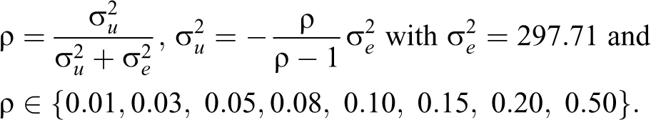
As noted above, since the data are assumed to take a multilevel structure (units inside areas), the ICC will have relevance and requires sensitivity testing. The ICC varies across applications dependent upon the extent to which the variability in the data observes a hierarchal structure with, for example, values ranging across 0.005, 0.05, and 0.2 with respect to mortality (Ambugo and Hegn, 2015), fear of crime (Whitworth 2012), and well-being (Moretti et al. 2019), respectively. Given that the ICC plays a role in the performance of the model-based MSE estimator, it is important that sensitivity tests are performed around its value within the simulation (Molina, Nandram, and Rao 2014; Moretti et al. 2018). We use the following relationships to explore the role of the ICC in the case of the Normal distribution:
Due to space constraints, in the cases of the Gumbel and Logistic distributions, the ICC is set at a realistic value of 0.05 only (see, e.g., Moretti et al. 2019).
In order to produce the small area IPF estimates, we create the following classes identifying the benchmark constraints related to the covariates x 1 and x 2:


Simulation Steps
The simulation consists of the following steps: Population generation: Generate the responses Draw a stratified random sample with simple random sample without replacement selection in each area d from each simulated population, Estimate Estimate Estimate the MSE of
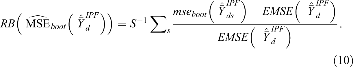
In order to evaluate the performance of the proposed bootstrap MSE estimator, the following quality measures are calculated:
Empirical MSE of

Empirical MSE of

Relative bias of
Relative bias of
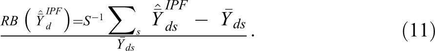
Relative bias of
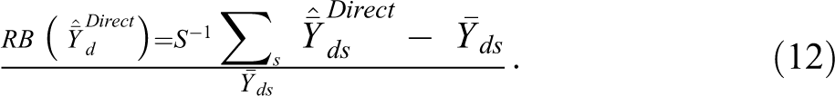
where
In the following section,
Results
Performance of the bootstrap MSE estimator under different distributional assumptions of
(
)
Figure 2 presents the empirical root MSE (ERMSE) of the IPF estimator and the direct estimator. Since the performance is very similar across all three distributions, Figure 2 presents the findings for the Normal case only, ordered by increasing small area sample size.
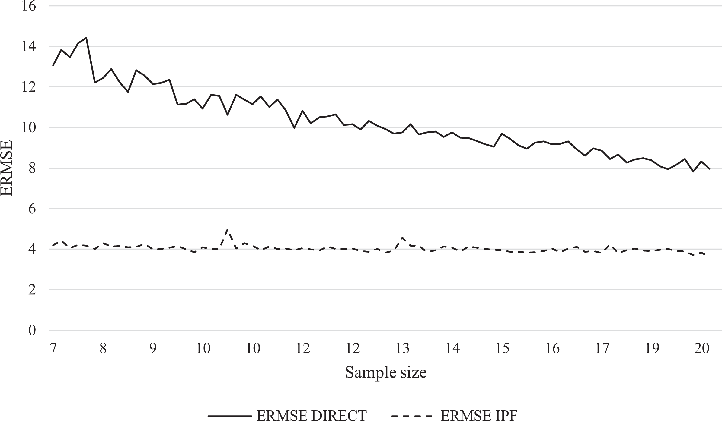
Empirical root mean squared error comparisons: Direct versus iterative proportional fitting estimator for the Normal case.
It can be seen that the IPF synthetic estimator provides estimates with lower MSE than the direct estimator due to the use of related auxiliary variables in reducing variance. This is particularly true for small areas with smaller survey sample sizes where the performance gains of IPF are large relative to direct estimator. This occurs because the ERMSE of the direct estimator naturally depends on the survey sample size: When the survey sample size in the small area d is smaller, the ERMSE tends to increase due to the larger variance around such estimates. As the small area survey sample size increases, the performance gains of the synthetic IPF estimator decline relative to the direct estimator until a point where its performance converges with that of the direct estimator. For reference, Figure 2 looks identical when ordered by sampling fraction rather than sample size.
For each distribution, Figure 3 shows the IPF point estimates across the small areas plotted against the true values observed in the population.
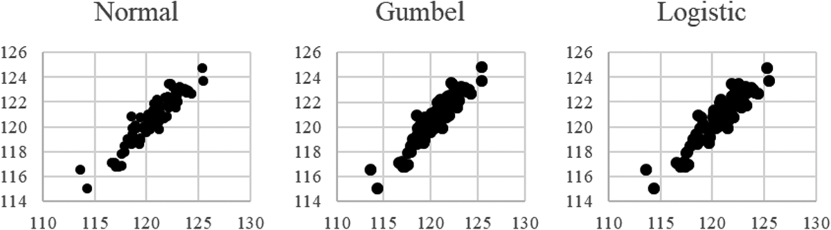
Comparisons of iterative proportional fitting estimates versus true means.
Table 1 shows the median estimate comparisons obtained using
Point Estimates Comparisons and Relative Biases Across the Small Area, Median Values Where Intraclass Correlation = 0.05.
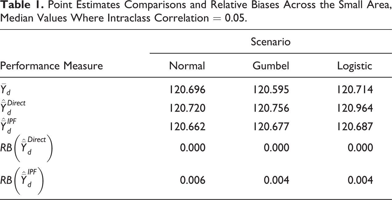
Figure 4 moves on to focus on the performance of the bootstrap MSE estimator to calculate the uncertainty around those central small area point estimates in the three Normal, Gumbel, and Logistic distributions, respectively. It can be seen that our proposed bootstrap approach provides nearly unbiased estimates of the true MSE with relative bias centered on and close to zero across the small areas. No association is found between estimate bias and sampling fraction across Figure 4.
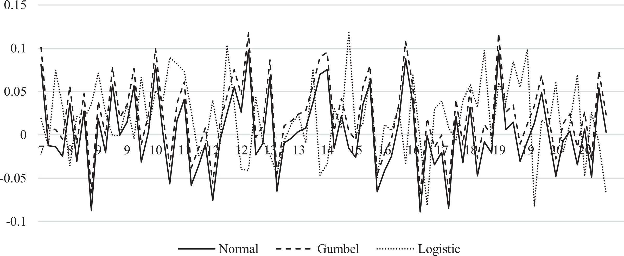
Table 2 provides further details of the performance of the bootstrap MSE estimator across the three distributions. In particular, the true MSE (i.e., empirical MSE) in each distribution is compared to our bootstrap MSE estimate and coverage rates (of 95 percent confidence intervals) are also presented. It can be seen that the relative bias values are close to zero and that the MSE bootstrap estimator is nearly unbiased across the small areas in each of the three distributions.
Performance Measures of the Bootstrap MSE Estimates.
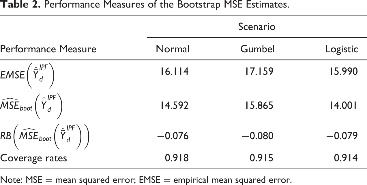
Note: MSE = mean squared error; EMSE = empirical mean squared error.
On the role of the ICC in the case of the Normal distribution
On the basis of these analyses, the performance of our proposed MSE estimator is encouraging in terms both of the small relative bias of the MSE estimates and the quality of the coverage. However, as noted above, it may be that the magnitude of the ICC affects the performance of the MSE estimator.
Table 3 shows the findings of ICC sensitivity analyses with a focus on the Normal distribution where the ICC is varied at several points from 0.01 to 0.50. The results for
Performance Measures of Our Bootstrap MSE Estimator at Varying Levels of Intraclass Correlation in the Normal Distribution.
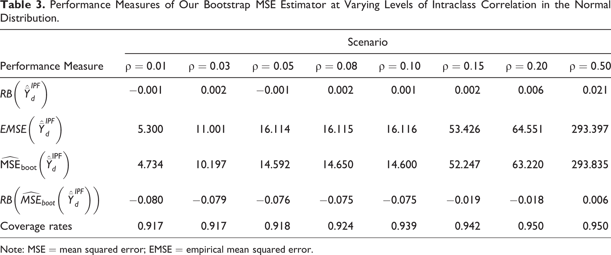
Note: MSE = mean squared error; EMSE = empirical mean squared error.
Application to Small Area Income Estimation in Italian Municipalities
This section provides a real-world application of an IPF small area estimator and, more centrally for this article, of our proposed bootstrap estimator of its MSE. The application used is the estimation of mean equivalized annual household disposable income (in Euros) for the municipalities of Tuscany region (
Model Fitting and Internal Validation
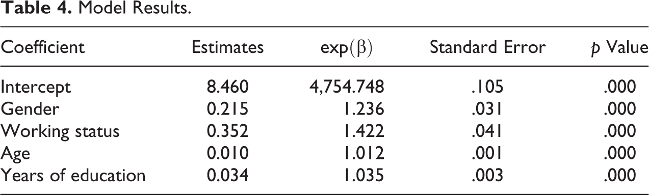
The explanatory variables used in this application are working status, years of education, gender, and age of the survey identified head of household. These have been informed by preliminary model investigations and findings from previous studies (Giusti et al. 2013). Model diagnostics identified some skewness and outliers in the distribution of the income outcome variable, as is common with such distributions, and this variable was therefore log transformed. No evidence of leverage was found. Table 4 presents the results from the log-linear linear model in EU-SILC based on (3).
Model Results.
Validation is an important step in any SAE study. SAE models can be validated internally in terms of the underlying model and externally against some known other external data of the target outcome variable. In terms of the internal validation, Figure 5 shows the fitted values versus the residuals as well as the Q–Q plots of the residuals from the log-linear model used to produce the MSE of the IPF estimates. These show good behavior with respect to the normality assumption. External validation is discussed below.
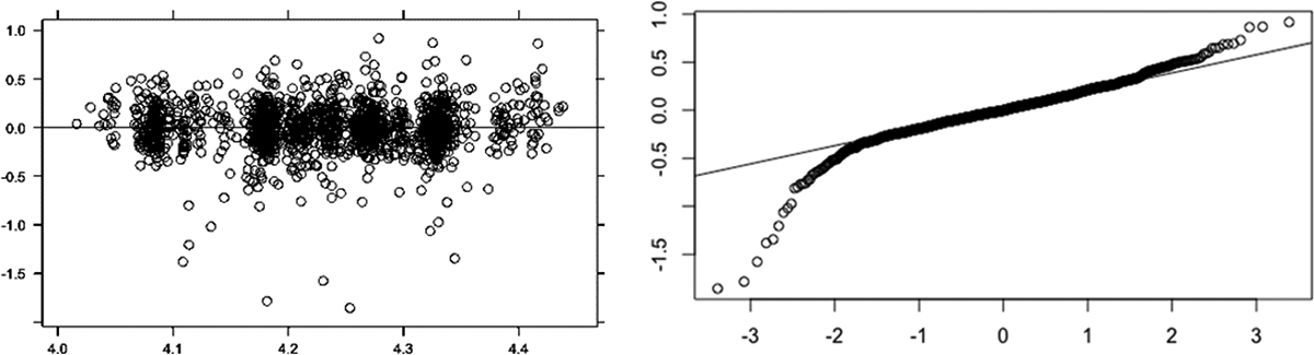
Fitted values versus residuals (left) and Q–Q plot of the residuals from the model used to produce the mean squared error of the iterative proportional fitting estimates.
Estimating Municipality Income in Tuscany
This section discusses the results of the IPF SAE of the mean equivalized annual household disposable income across Tuscan municipalities along with their uncertainty estimates. Figure 6 maps the mean IPF estimates across the 287 Tuscan municipalities. The map displays municipalities in four quartiles and shows a range in 2009 municipal income estimates from a low of just over 16,000 Euros per annum to a high of just under 20,000 Euros per annum. Municipalities located in the provinces of Massa Carrara (North West), Grosseto (South), and Prato and Pistoia (North) show the lowest estimated municipal income levels. On the contrary, municipalities around Florence, Arezzo, Pisa, and Livorno show the highest estimated municipal income levels.
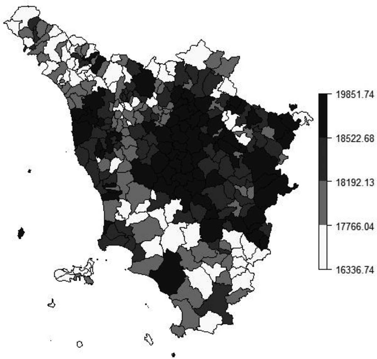
Iterative proportional fitting income estimates for Tuscan municipalities.
In terms of external validation of these IPF estimates, a frequent inherent challenge, as here, is the typical lack of any such existing small area data against which to validate (hence the motivation for the SAE). External validation of these IPF estimates is provided in two ways. Firstly, the spatial patterns in Figure 6 are in line with known geographical patterns of similar indicators across Tuscany seen in previously published research (Giusti et al. 2015; Moretti et al. 2019). Secondly, no identical income indicators exist at this municipality scale, and no direct survey estimates to municipality level are viable from the EU-SILC survey data. However, it is viable to produce direct survey estimates from the EU-SILC survey data to Tuscany’s 10 larger provinces and to compare these with indirect IPF estimates also to province level. The Spearman’s rank correlation between these two sets of estimates is.93, and this is statistically significant at below the 1 percent level, although acknowledging the limited sample size involved.
Table 5 presents summary statistics of the uncertainty of the direct survey estimates compared with the IPF estimates. In particular, it shows the root mean squared error (column 1) and, expressed as a percentage of the estimates, the relative root mean squared error (RRMSE%; column three) of the small area estimates. Given that the direct estimates are unbiased, the standard deviation (SD; column 2) and coefficient of variation (CV%; column 4) of the direct estimates enable a comparison of uncertainty of the direct estimates with the bootstrap MSE estimates of the IPF estimator. The coefficient of variation (CV) is a standardized measure of the dispersion of a distribution and is calculated as a ratio of its SD to its mean. In the present analyses, it is obtained as the ratio between the SD of the direct survey estimate and the direct survey estimate for every area. Since direct estimates are unbiased, their CVs represent measures of uncertainty (Rao and Molina 2015). RRMSE and CV are standard measures of uncertainty that are required in many official statistics institutes (see Schirripa-Spagnolo, D’Agostino, and Salvati 2018; Statistics Canada 2009).
Summary Statistics of the Performance Gains from the Synthetic IPF Estimator Compared to the Direct Estimator for Small Area Income Estimates Across Tuscan Municipalities.
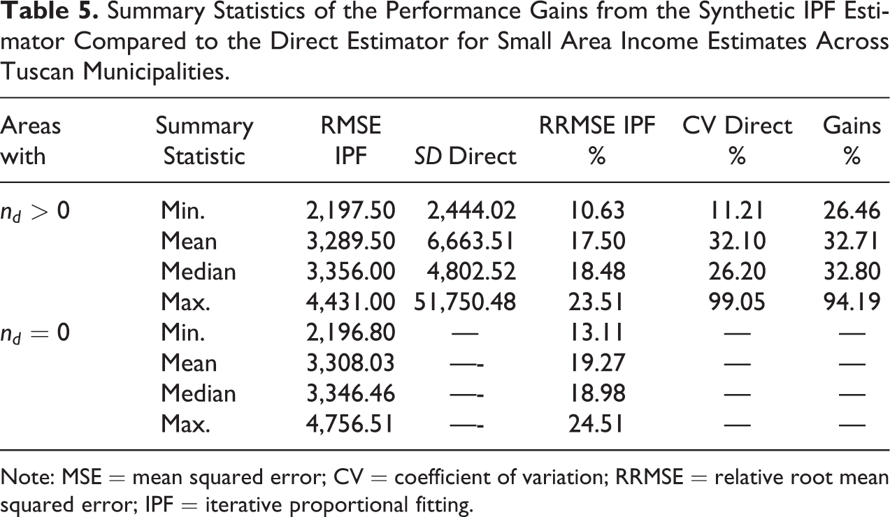
Note: MSE = mean squared error; CV = coefficient of variation; RRMSE = relative root mean squared error; IPF = iterative proportional fitting.
Table 5 shows that the IPF estimates are more reliable than the direct estimates across all points of the income distribution, as depicted by the lower values of the RRMSE IPF (column 1) and RRMSE IPF (column 3) compared to SD direct (column 2) and CV direct (column 4), respectively. The IPF small area estimates can also be considered reliable in absolute terms. Values of RRMSE below a threshold of 20 percent are often taken by statistical agencies as acceptable (Commonwealth Department of Social Services 2015), and almost all of this municipality distribution of small area estimates is below this level. The final column of Table 5 summarizes the gains in efficiency of the IPF estimates over the direct survey estimates by comparing the MSE for the IPF estimator with the variance of the unbiased direct estimator. Technically, these are calculated by
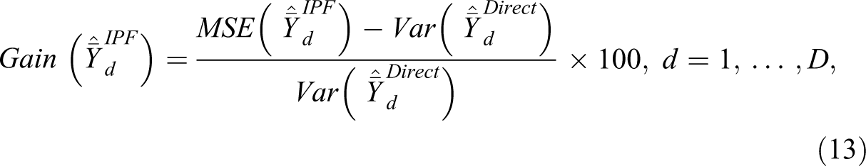
where
Figure 7 drills down to focus on the extent to which these performance gains vary according to the size of the municipality sample size in the EU-SILC survey, a key driver of the variance of the direct estimator and key limiter of the viability of using the direct estimator to produce reliable survey estimates for small areas. To aid comparison, Figure 7 is ordered from left to right by municipality survey sample size in the EU-SILC. RRMSE is shown for the IPF estimates, while CV is shown for the direct estimates. Figure 7 illustrates that the RRMSE of the indirect IPF estimates does not depend on the sample size in contrast to the direct estimator. As such, Figure 7 highlights that while performance gains from the IPF estimator are seen across the whole distribution, they increase as the municipality sample size in the survey decreases. Among those municipalities with the smallest survey sample sizes, there is a marked increase in the performance gains available from the IPF estimator compared to the direct survey estimator. Figure 7 is naturally only able to display comparative results for municipalities with nonzero sample sizes, given that direct estimates cannot be produced for small areas with zero sample size. Estimates for these municipalities do of course become viable with synthetic IPF estimator. For reference, Figure 7 looks identical when ordered by sampling fraction rather than sample size.
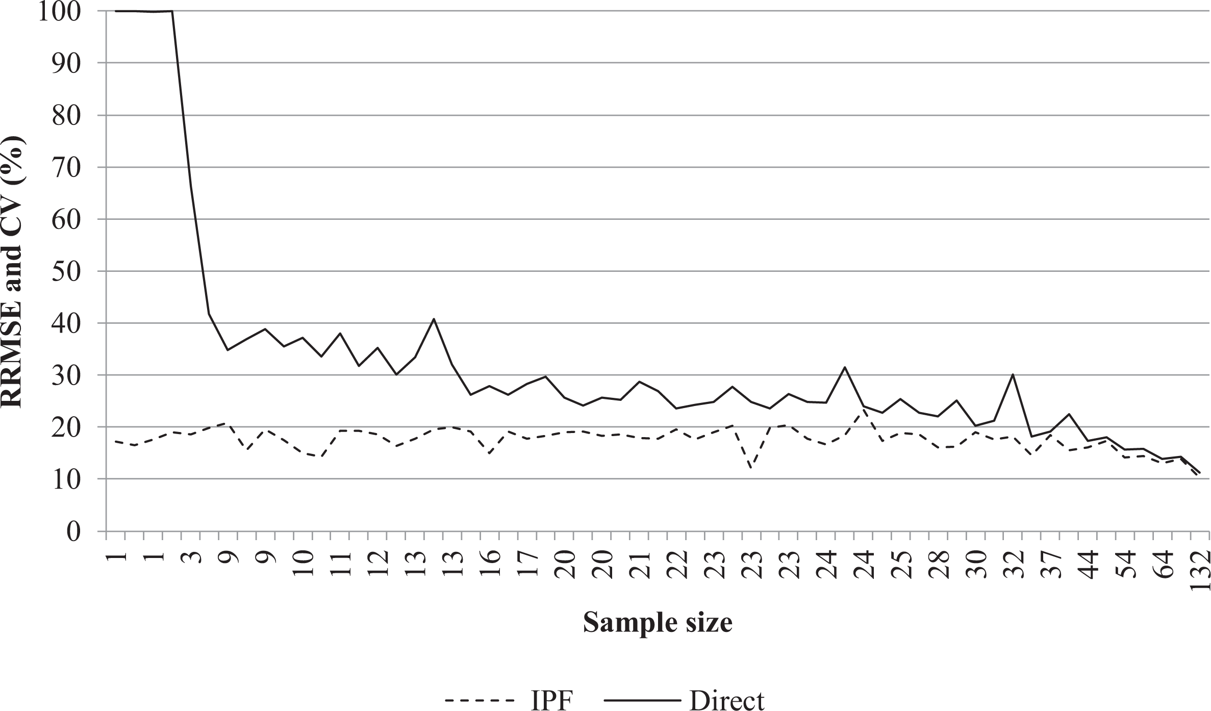
Performance comparison sorted by small area sample size.
Discussion
The combination of high costs of survey data collection and increasing demands for ever more spatially detailed data from policy makers and scholars alike mean growing demands for SAE techniques. Spatial microsimulation approaches to SAE continue to be widely used across diverse domains including transport, health, physical activity, and income. However, their continuing inability to produce reliable estimates of uncertainty alongside their central point estimates remains a pressing limitation to their utility for practitioners and scholars alike. This is understandable in part given that the estimation of MSE is difficult in a spatial microsimulation context since it cannot be estimated in a closed form and analytical approximations are highly challenging.
Widely discussed in the SAE literature is the importance of providing measures of uncertainty such as MSE or confidence intervals alongside the central point estimates in order to assess the reliability of the small area estimates (Pratesi 2016). This is particularly important where policy decisions are taken on the basis of the small area estimates since the consequences of real-world decision making without a clear sense of the uncertainty around the point estimates can be misleading and potentially harmful (Goedemé et al. 2013). Klevmarken (2002:264) argues that “[T]he credibility of [microsimulation models] with the research community as well as with users will in the long run depend on the application of sound principles of inference in the estimation, testing and validation of these models.”
This article provides a significant development in this context by presenting a novel parametric bootstrap approach for the estimation of uncertainty in spatial microsimulation SAE techniques. Importantly, the measure of uncertainty estimated is the MSE that contains both the variance and bias of the estimate. Simulation results demonstrate that under model assumptions, our proposed MSE estimator is relatively unbiased and displays good coverage properties against known true population values. The approach delivers substantial performance gains compared to the direct estimator across all portions of the distribution. In doing so, our approach enables researchers and policy makers alike to quantify both the performance gains potentially available through the use of spatial microsimulation approaches to SAE compared to direct survey estimates and to quantify the extent of uncertainty around those small area estimates. The simulation results show that those performance gains exist irrespective of the target small area sample size but are especially large at low sample sizes (below 10 in this simulation) and, naturally, when small areas have zero sample size such that direct estimates are nonviable but synthetic small area estimates are possible. Sensitivity tests confirm that these performance gains are maintained both across nonnormal Gumbel and Logistic distributions as well as across differing values of ICC, though coverage performance falls slightly at very low levels of the ICC in our simulation. A practical data application using EU-SILC data to municipality income across Tuscany is presented and validated in order to demonstrate the applicability and similar performance of the MSE bootstrap estimator in a real-world setting.
While the performance and sensitivity analyses confirm that our proposed approach evaluates well and marks a significant contribution to the field, it serves also to open up opportunities for further more advanced enquiry as a result. First, we focus here only on a linear model. Future work will need to explore the performance of other nonlinear models in this context. However, the bootstrap approach in these scenarios will follow the same steps as those proposed in our approach. Second, a clear next step is to extend the framework to different types of outcome variables beyond the scalar target variable assessed here. Third, in this study, the common case of nonnormal error terms is assessed, and our simulation study shows good performance of the MSE estimator in distributions with mild skew and heavy tails as well as in the normal case. However, future work could take into account more fully the implications of and potential responses to failures in model assumptions and of model failure. Our hope therefore is that this article’s contributions will not only make a significant advance to research and policy practice in spatial microsimulation SAE, but that it will also stimulate further scholarly attention to these and other areas.
Supplemental Material
Supplemental Material, sj-docx-1-smr-10.1177_0049124120986199 - Estimating the Uncertainty of a Small Area Estimator Based on a Microsimulation Approach
Supplemental Material, sj-docx-1-smr-10.1177_0049124120986199 for Estimating the Uncertainty of a Small Area Estimator Based on a Microsimulation Approach by Angelo Moretti and Adam Whitworth in Sociological Methods & Research
Footnotes
Declaration of Conflicting Interests
The author(s) declared no potential conflicts of interest with respect to the research, authorship, and/or publication of this article.
Funding
The author(s) disclosed receipt of the following financial support for the research, authorship, and/or publication of this article: This work was supported by the UK Economic and Social Research Council National Centre for Research Methods (grant number ES/N011619/1).
Supplemental Material
Supplemental material for this article is available online.
References
Supplementary Material
Please find the following supplemental material available below.
For Open Access articles published under a Creative Commons License, all supplemental material carries the same license as the article it is associated with.
For non-Open Access articles published, all supplemental material carries a non-exclusive license, and permission requests for re-use of supplemental material or any part of supplemental material shall be sent directly to the copyright owner as specified in the copyright notice associated with the article.