Sage Journals: Discover world-class research

Abstract

American cities and neighborhoods vary in their residents’ typical levels of mental health. Despite scholarship emphasizing that we cannot thoroughly understand city and neighborhood problems without investigating how they are intertwined, limited research examines how city and neighborhood effects interact as they impact health. I investigate these interactions through a study of the effects of the Great Recession of 2007–2009. Using Waves 1 (2005–2006) and 2 (2010–2011) of the National Social Life, Health, and Aging Project survey (N = 1,341) and in accordance with the compound disadvantage model, I find through fixed-effects linear regression models that city- and neighborhood-level economic declines combine multiplicatively as they impact older Americans’ depressive symptoms. I furthermore find that this effect is only partly based on personal socioeconomic changes, suggesting contextual channels of effect. My results show that we cannot fully understand the effects of city-level changes without also considering neighborhood-level changes.

Keywords

depressive symptoms economic decline city neighborhood socioeconomic status aging

Introduction

American cities and their neighborhoods vary substantially in the typical levels of mental health of their residents. In 2005, Midland–Odessa, TX’s average citizen experienced 2.2 days of depression per month. The corresponding amount was 3.4 in Bloomington, IN, and 4.5 in Santa Rosa-Petaluma, CA (Sperling and Sander 2007). This points to how social, cultural, demographic, economic, and political features of cities impact their residents’ well-being (Galea, Freudenberg, and Vlahov 2005). Features of neighborhoods also impact the health and life satisfaction of their residents; these include social cohesiveness (Cramm, van Dijk, and Nieboer 2013; Feldman and Oberlink 2003); prevalent health practices (Dragano et al. 2007); extent of urbanization; degree of segregation based on marital status, age, and ethnicity (van Hooijdonk et al. 2007); and the extent of disadvantage, disorder, and disorganization (Bursik 1988; Sampson and Groves 1989). Scholarship shows that neighborhoods within the same city can vary extensively in their physical, demographic, social, economic, and political features (e.g., Pearce, Witten, and Bartie 2006; Rundle et al. 2007).

This research encourages study of how both city and neighborhood contexts impact residents. While much research has studied cities and neighborhoods as independent influences on health and well-being, scholars have argued that in addressing population health and social issues, research must build bridges between the numerous levels of analysis (Kaplan, Everson, and Lynch 2000; van Kempen, Bolt, and van Ham 2016). Accordingly, van Kempen et al. (2016) emphasized that neighborhood problems and their solutions can only be understood by examining how neighborhoods are intricately linked with their cities’ policies, processes, and circumstances, all of which strongly impact neighborhoods’ social and economic conditions (Kaplan et al. 2000; van Kempen et al. 2016). Nonetheless, relatively few scholars have investigated how city- and neighborhood-level variables interact as they affect residents’ health (e.g., Acevedo-Garcia et al. 2003; Diez Roux 2001; Galea et al. 2005; Pemberton and Humphris 2016). This study is unique as it examines how city-level economic declines through an economic shock, the Great Recession of 2007–2009, interact with declining neighborhood conditions in influencing the depressive symptoms of older residents.

Present-day demographic trends motivate the study of how cities and their neighborhoods impact older persons. Caused by declining rates of fertility and rising life expectancies, population aging is an important demographic trend across the industrialized world (Brown 2011; Cooke 2006; McDaniel and Rozanova 2011; McDonald and Donahue 2011; Turcotte and Schellenberg 2007). Furthermore, these aging populations are increasingly living within cities, making aging an important urban phenomenon. The numerical significance of older adults has thus increased. Accordingly, older adults’ engagements in paid work, community activities, and social life more generally have acquired greater importance. As healthier and happier older adults are more involved in paid employment (e.g., Austen and Ong 2009; van den Berg, Elders, and Burdorf 2010; van Rijn et al. 2014) and in community groups and activities (Cornwell, Laumann, and Schumm 2008; Kohli, Hank, and Kunemund 2009; Young, Russell, and Powers 2004), there is an increasing need to comprehend how cities and their neighborhoods affect older adults’ mental health.

Furthermore, the physical and cognitive declines that often co-occur with aging might increase older persons’ susceptibility to negative features of their environments (Lawton and Nahemow 1973). This vulnerability might be intensified by older adults’ higher spatial confinement, caused by retirement, functional health problems, or other life course events, transitions, and circumstances (Choi et al. 2015; Glass and Balfour 2003; Krantz-Kent and Stewart 2007). The physical and social circumstances of neighborhoods might therefore have a stronger influence on older residents (Lawton and Nahemow 1973). These aging processes provide additional reasons for why it is particularly important to understand how cities and their neighborhoods affect the health and well-being of their older residents.

The Great Recession was a difficult experience for many older Americans (Boen and Yang 2016; Cagney et al. 2014). Between 2007 and 2011, more than 1.5 million older Americans underwent home foreclosure (Trawinski 2012). While any individual older person’s absolute risk of home foreclosure might have remained relatively low, apprehension caused by increased risk of home foreclosure within one’s immediate environment can be consequential for well-being (Cagney et al. 2014). Between 2007 and 2010, the median family net worth of heads of households from 55 to 64 years of age dropped by almost one third, whereas that of those from 65 to 74 years of age dropped by about 18 percent (Ackerman, Fries, and Windle 2012). Almost one out of every four adults above the age of 50 stated that they had depleted their savings to endure the difficulties of the recession (Rix 2011).

Background

Theoretical Perspectives

I use the compound disadvantage model as an orienting framework. In its most abstract formulation, this model proposes that “The effects of separate sources of disadvantage of the same type combine multiplicatively . . .” (Wheaton and Clarke 2003:695). While this model has mostly been applied to disadvantaged people within disadvantaged neighborhoods (Gilster 2014; Wheaton and Clarke 2003; Wodtke, Elwert, and Harding 2016), the concept of multiplicative effects of diverse sources of the same type of disadvantage is applicable to neighborhood conditions within cities. I examine interactions between measures of economic health and stability at the city and neighborhood levels, thereby presenting an ecological compound disadvantage model.

Disadvantaged city and neighborhood conditions can affect residents’ depressive symptoms through numerous pathways. Declining cities often show higher rates of home foreclosures, producing externalities at the neighborhood level that decrease the upkeep, maintenance, and values of homes while increasing levels of crime and disorder (Leonard and Murdoch 2009). Urban neighborhoods in decline show high extents of vandalism, delinquent activity, and unrestrained young persons, all of which are stressful and cause fear. These stressors lead residents to avoid leaving their homes and becoming involved in community activities and to restrict their interactions to close family members and friends (Aneshensel 2010; Aneshensel et al. 2011). These constraints are damaging to mental health (Aneshensel 2010). Moreover, city- and neighborhood-level economic declines lead to the erosion of personal wealth and income (Boen and Yang 2016; Meltzer, Steven, and Langley 2013), creating financial strains and stressors that damage health (Boen and Yang 2016; Hajat et al. 2010, 2011; Pool et al. 2017; Robert and House 1996). These financial difficulties are partly based on rising rates of unemployment in American cities and neighborhoods undergoing socioeconomic declines (Chatterjee and Eyigungor 2015; Katz, Wallace, and Hedberg 2013; Zivin, Paczkowski, and Galea 2011). As such, worsening circumstances within cities and their neighborhoods might affect depressive symptoms in an additive fashion; each one might impact mental health net of the other. Furthermore, their effects might occur through losses in personal socioeconomic status and through contextual channels.

Beyond additive effects, an ecological compound disadvantage model postulates that city- and neighborhood-level economic declines will combine multiplicatively as they impact residents’ mental health. A possible mechanism for a multiplicative combination of city- and neighborhood-level effects is presented by Baumer, Wolff, and Arnio (2012), who discussed disadvantaged neighborhoods within “vulnerable” cities marked by extensive socioeconomic difficulties. In their analysis of the Great Recession, they stated that declining neighborhoods embedded within larger political contexts in which resources are sparse are less able to obtain needed resources, such as for foreclosure mitigation and for the maintenance and repurchasing of abandoned buildings. Similarly, Allen (2013) discussed how declining property values and incomes through the recession reduced cities’ tax revenues, impairing cities’ provision of services to their neighborhoods, including for the upkeep of streets and abandoned buildings.

These multiplicative effects on older residents’ depressive symptoms likely come about through both negative changes in features of contexts and personal financial problems. Increased home foreclosures and detriments to the quality of streets and properties create neighborhood-level externalities that reduce the values of homes and raise extents of disorder and criminal activity (Leonard and Murdoch 2009). As housing prices form large proportions of Americans’ total net worth (De Nardi, French, and Benson 2012), these negative externalities impact Americans’ total household assets. Furthermore, availability of financial resources is key to the stimulus packages enacted at the federal, state, city, and municipal levels to counteract the effects of the Great Recession (Dethier and Morrill 2012; Miller and Hokenstad 2014). Stimulus spending can invigorate declining neighborhoods through improving employment circumstances, raising spending, and increasing residents’ incomes. These effects are pertinent to older residents’ households’ financial circumstances as the economic challenges of the Great Recession forced many older Americans to delay their retirement plans (Munnell and Rutledge 2013). Furthermore, older Americans commonly co-reside with younger family members (see Russell 2009; Ulker 2008) who are likely to work for pay. Accordingly, the negative effects of residing within a city with weakening resources might be accentuated within neighborhoods undergoing increasing disadvantage and need for additional resources.

In examining these contextual effects, I focus on depressive symptoms. Depression is a central psychological outcome of stressful circumstances, as well as an all-round indicator of stress (Pearlin 1989; Pearlin, Aneshensel, and LeBlanc 1997; Pearlin et al. 1981). Among older adults, depression might be the most prevalent form of emotional suffering (Blazer 2003). In later life, depression is a strong predictor of suicide (Blazer 2003; Fiske, Wetherell, and Gatz 2009; Vanderhorst and McLaren 2005) and is linked to higher morbidity, detriments to cognitive, social, and physical functioning, and self-neglect, all of which are associated with mortality (Blazer 2003; Fiske et al. 2009).

The Great Recession of 2007–2009

I study the interactive effects of declining city and neighborhood conditions within the context of the Great Recession of 2007–2009, which was the most extensive global economic crisis since the 1930s’ Great Depression (Meltzer et al. 2013). This economic shock involved the collapse of the property market, leading to immense losses within the financial sector and culminating in a pronounced recession during which the typical American family lost approximately 40 percent of its net worth. Furthermore, the United States underwent its greatest declines in gross domestic product and levels of employment since the Great Depression (Meltzer et al. 2013). Economic challenges through this recession, including increased rates of home foreclosures, have been associated with lower well-being (Cagney et al. 2014; Houle 2014) and higher rates of suicide (Houle and Light 2014). Similarly, declining incomes (Burgard, Seefeldt, and Zelner 2012) and rising levels of unemployment (Phillips and Nugent 2014) through this recession harmed physical and mental health. In addition, those who lost substantial amounts of their housing wealth through this recession underwent high levels of stress (Yilmazer, Babiarz, and Liu 2015).

Despite the scope of the recession, American cities varied extensively in how hard they were hit. While some cities achieved a rapid and successful recovery (e.g., San Jose and San Francisco), other cities remain in troubled circumstances (e.g., Tampa and Orlando) (Arias, Gascon, and Rapach 2016; Davidson 2014; Dill 2014; Gray and Scardamalia 2014). Traits of cities that fared better through the recession include the possession of larger and more educated populations as well as economies less dependent on real estate (Arias et al. 2016; Florida 2016; Gray and Scardamalia 2014). While cities within the South and West census regions fared the worst economically through the recession, those in the Midwest underwent less potent economic declines, and those in the Northeast fared the best (Hacker et al. 2012). These regional variations are linked with differences in racial/ethnic composition, percentages of heads of households who hold high school diplomas and college degrees, and employment rates (Hacker et al. 2012).

Cities most impacted by the recession underwent substantial decreases in the prices of homes (Arias et al. 2016; Chatterjee and Eyigungor 2015; Gray and Scardamalia 2014) and overall levels of income (Chatterjee and Eyigungor 2015; Katz et al. 2013; Zivin et al. 2011). Both median home prices (see Chatterjee and Eyigungor 2015; Diamond 2017; Kahn 2017; Lutz 2008) and median household incomes (see Brasier et al. 2011; Chatterjee and Eyigungor 2015; Jha 2017; Maher and Deller 2011) are central determinants of tax revenues, affecting the resources that a city can channel into needy neighborhoods and dedicate to citywide public goods and services. As such, city-level median home prices and median household incomes are highly pertinent to this study.

There is also substantial evidence of the recession having affected people’s well-being through their neighborhoods. Neighborhood-level home foreclosure rates were linked with significant depressive symptoms (Cagney et al. 2014). Neighborhoods undergoing housing instability showed high levels of stress, homelessness, and residential crowding, as well as higher risks of illness due to abandoned buildings that accumulated insects and other disease carriers (Burgard and Kalousova 2015).

While most American urban neighborhoods were economically affected by the recession (Owens and Sampson 2013; van Kempen et al. 2016; Zwiers et al. 2016), there was considerable variability within cities. Neighborhoods that were disadvantaged pre-recession tended to be more heavily impacted (Grusky, Western, and Wimer 2011; Owens and Sampson 2013; van Kempen et al. 2016; Williams, Galster, and Verma 2013), as were communities in which minority racial groups and immigrants were concentrated (Downing 2016; Owens and Sampson 2013; Williams et al. 2013). Larger cities contain neighborhoods that are more economically and racially segregated (David 2018; Florida 2015; Florida and Mellander 2015; Kent and Frohlich 2015; Nodjimbadem 2017; Wilson 2017). As such, their neighborhoods showed higher variability in how they fared through the recession. Cities of higher affluence and with more high-tech and knowledge-based economies also show greater neighborhood economic segregation (Florida 2015; Florida and Mellander 2015). This increased intra-city variability in their neighborhoods’ economic fortunes during and after the recession.

Accordingly, neighborhood disadvantage shifted systematically through the Great Recession, in varied ways across cities, supporting the study of disadvantage across neighborhoods and cities. Each city neighborhood potentially presents a unique configuration of city- and neighborhood-level economic changes, yielding a unique effect on residents’ well-being. This presents the possibility that there are multiplicative effects between city- and neighborhood-level economic changes that would be obscured by a merely additive analysis.

Research Question and Hypothesis

In this study, I investigate whether increased neighborhood-level need accentuated the impact of declining city-level resources through the Great Recession on residents. I also test whether this effect is mostly based on personal financial changes or whether changes to features of contexts are also important channels of effect. Based on an ecological compound disadvantage model, I hypothesize that declining resources at the city level interact with worsening neighborhood conditions in influencing older residents’ depressive symptoms. I further hypothesize that only a portion of this effect is based on personal socioeconomic declines; changing socioeconomic features of contexts in themselves affect depressive symptoms.

Data and Method

Data Set and Sample

I use the National Social Life, Health, and Aging Project (NSHAP) survey (Wave 1: Waite et al. 2014-b; Wave 2: Waite et al. 2014-a) as a source of individual-level variables. The NSHAP follows a representative sample of older Americans through time, and its variables focus on social relationships, health, and well-being. This data set is developed through a complex multistage area probability sampling design that comprises 58 cities (specifically, metropolitan statistical areas [MSAs]) that substantially vary in how they fared during and after the Great Recession. I tied respondents with their MSAs and neighborhoods (specifically, census tracts) using protected geodata I procured via special contractual arrangements from the National Opinion Research Center. I analyze the subsample of NSHAP respondents who remained within the same MSA between Waves 1 and 2 (further explained below). Suzman (2009) and O’Muircheartaigh, Eckman, and Smith (2009) provided further details concerning the sampling design employed in the NSHAP. At Wave 1 (2005–2006), 3,005 respondents between the ages of 57 and 85 years were interviewed. The Wave 1 response rate was 75.5 percent, and 75.2 percent of Wave 1 respondents were reinterviewed at Wave 2 (2010–2011). The rate of retention between Waves 1 and 2 (76.0 percent) was comparable for those NSHAP respondents dwelling within MSAs at the time of the first wave. This data set is particularly useful as the timing of Waves 1 and 2 allows me to study the effects of the Great Recession of 2007–2009.

I study only those NSHAP respondents who remained within the same MSA between Waves 1 and 2. This is because I am investigating how economic changes within cities through the recession interacted with worsening neighborhood circumstances in affecting older residents’ depressive symptoms. Of the 3,005 NSHAP respondents at Wave 1, 2,073 dwelled within MSAs. By Wave 2, 731 respondents (of the 2,073 MSA residents at Wave 1) had either dropped out of the NSHAP sample (n = 397) or moved to a new MSA (n = 334). The number of respondents per MSA ranges from 1 to 61, the average being 23.14. The analytical sample includes 1,342 respondents.

In some regards, respondents living in MSAs at Wave 1 (n = 2,073) were similar to those not initially residing within MSAs (n = 932). These two groups did not differ statistically according to gender and mental health. However, those initially dwelling within MSAs were younger, more racially/ethnically diverse, of better physical health, wealthier, and more educated and were more likely to be married or living with a partner, to be employed, to view themselves as being of higher social status, and to be residing within a neighborhood of lower concentrated disadvantage.

Among Wave 1 MSA-dwelling respondents (n = 2,073), those who remained within the analytical sample at Wave 2 (n = 1,342) did not differ in some respects from those who did not (n = 731). These two groups did not differ according to gender, race/ethnicity, total household assets, and self-assessment of social class. However, those who remained in the sample (n = 1,342) tended to be younger, more educated, and healthier and were more likely to be married or living with a partner, as well as to be working for pay. Respondents who remained within the analytical sample (n = 1,342) also tended to reside within MSAs that at Wave 1 had lower median household incomes, median home prices, and rates of foreclosed homes. Furthermore, retained respondents (n = 1,342) tended to reside at Wave 1 within census tracts with higher initial concentrated disadvantage.

As regards education, health, relationship status, and employment status, Wave 1 respondents who did not remain within the analytical sample show disadvantages compared with those who did. Accordingly, if those more susceptible to depressive symptoms had lower likelihoods of remaining within the analytical sample, attrition between Waves 1 and 2 might lead to conservative assessments of how contexts undergoing economic declines affect their residents’ depressive symptoms.

Dependent Variable

I study depressive symptoms through an index that combines 11 symptoms of depression with an assessment of general happiness. The former are based on an 11-item short-form version of the 20-item Center for Epidemiologic Studies Depression Scale (CES-D). Respondents reported on the extent to which they felt everything was an effort, they felt depressed, their sleep was restless, they felt lonely, they enjoyed life, and so on over the past week. They responded to each question on an ordinal scale spanning from (1) rarely or none of the time to (4) most of the time. I reverse-coded two of these 11 measures so that all items indicate increasing levels of depressive symptoms. I assess general happiness through the question, “If you were to consider your life in general these days, how happy or unhappy would you say you are, on the whole?” Respondents answered on an ordinal scale spanning from (1) unhappy usually to (5) extremely happy. I reverse-coded this measure to fit with the direction of the other 11 measures.

In a study using the NSHAP, Payne et al. (2014) showed how, among older adults, these 12 items constitute a single cluster of mental health, and thus may be part of the same dimension of mental health. Congruently, I found through exploratory factor analyses (EFAs) that these 12 measures fit into one factor at both waves (according to the Kaiser criterion). This suggests that they are all indicative of the same aspect of mental health. To create this factor, I averaged standardized scores on all 12 measures, separately at Waves 1 and 2 (see Payne et al. 2014). At both waves, this index of depressive symptoms has high internal reliability (Cronbach’s alpha scores >.70). The standardized measure of general happiness I use is highly correlated at both waves with the 11 standardized measures of depressive symptoms from the CES-D. Results were substantively the same when I used an index of depressive symptoms based only on the 11 CES-D measures.

Independent Variables

MSA level

At the city level, I study MSAs. This is effective because MSAs approximate housing markets (Houle and Light 2017; Iceland, Weinberg, and Steinmetz 2002). Furthermore, their social and economic integration (U.S. Census Bureau 2016) implies that they approximate labor markets. An MSA is defined as

the county or counties (or equivalent entities) associated with at least one urbanized area of at least 50,000 population, plus adjacent counties having a high degree of social and economic integration with the core as measured through commuting ties. (U.S. Census Bureau 2016)

I focus on an index of resources based on median home prices and median household incomes. I obtained data for these two measures from the U.S. Census Bureau—American FactFinder (2017), which accumulated this information through the American Community Survey (ACS) (Wave 1: 2005 ACS; Wave 2: 2010 ACS). I adjusted both measures at Wave 1 for inflation to ensure the accuracy of comparisons with amounts at Wave 2. Based on the U.S. Bureau of Labor Statistics—CPI Inflation Calculator (Consumer Price Index Inflation Calculator 2017), I multiplied 2005 monetary amounts by 1.11652. To correct the right skew of both variables, I log-transformed them at both waves. Beyond normalizing their distributions, log-transforming these variables allowed me to study nonlinear associations with depressive symptoms; the natural logarithm of a continuous variable allows that variable to be analyzed in terms of ratios rather than absolute differences. These two logged variables were then standardized and averaged, producing the index of MSA-level resources. The Cronbach’s alpha for this index is over .80 at both waves. I also analyze logged MSA-level median home prices and logged MSA-level median household incomes separately to assess whether one of these two measures is the central driver of the results found for the index of MSA-level resources.

I study two additional measures of MSA-level economic circumstances: percentage unemployed and percentage of homes foreclosed. Increases in rates of unemployment (Meltzer et al. 2013; Zivin et al. 2011) and rising rates of home foreclosures (Chatterjee and Eyigungor 2015; NBC News 2012; Wang and Immergluck 2018) are two other important dimensions of economic decline through the Great Recession. I obtained unemployment data from the U.S. Bureau of Labor Statistics—Local Area Unemployment Statistics (2017). I procured foreclosure data pertaining to 57 of the 58 MSAs I investigate from ATTOM Data Solutions (N.d.). It was not possible to obtain foreclosure information for one of these 58 MSAs. For this reason, analyses involving rates of home foreclosures are based on 19 fewer respondents. Percentages of homes foreclosed include homes in any phases of the foreclosure process (pre-foreclosure, auction, and bank-owned [or real estate owned]). Because these two variables are less direct measures of MSA-level resources, I appended them to my main focus. I include them to address the question of whether my results are based on changes in MSA-level resources specifically or MSA-level economic declines more broadly.

Census tract level

At the neighborhood level, I study census tracts, which are defined as

small, relatively permanent statistical subdivisions of a county or equivalent entity . . . . Census tracts generally have a population size between 1,200 and 8,000 people, with an optimum size of 4,000 people. A census tract usually covers a contiguous area; however, the spatial size of census tracts varies widely depending on the density of settlement . . . . Census tract boundaries generally follow visible and identifiable features. (U.S. Census Bureau 2012)

Census tracts have often been employed as effective approximations of neighborhoods (e.g., Estabrooks, Lee, and Gyurcsik 2003; LaVeist and Wallace 2000; Morland et al. 2002). For Wave 1, I used data from the 2000 Decennial Census. For Wave 2, I used data from the 2006–2010 ACS. Concerning the latter, data for each year from 2006 to 2010 were averaged because there were not enough respondents per census tract in each individual year. I accessed both sources of data through the U.S. Census Bureau—American FactFinder (2017).

I study an index of census tract-level concentrated disadvantage, developed by Sampson, Raudenbush, and Earls (1997). I use this index to operationalize neighborhood-level need for resources, and it is based on the percentage of the population below the poverty line, of households on public assistance, of female-headed households, of individuals unemployed, of individuals less than 18 years of age, and of individuals who are nonwhite. EFAs revealed that at both waves, these six items were best combined into one factor (according to the Kaiser criterion) and further provided factor loadings for each of these six items at each wave. Factor loadings indicate the strength of the association between each item and the underlying factor, and I employed them in developing the index of census tract-level concentrated disadvantage (explained below). A confirmatory factor analysis revealed that the factor structure of these six items significantly differed across the two waves; a factor structure refers to the set of correlations that exist among a set of variables used to construct an underlying factor. However, results were substantively the same when I employed the first or second wave factor loadings. For this reason, I only report results based on the Wave 1 factor loadings. I created this index by standardizing each of the six variables, multiplying each of the six standardized variables by its factor loading from Wave 1, and then averaging these six scores, separately at each wave. At Wave 1, this index had a Cronbach’s alpha of .91, whereas at Wave 2, the Cronbach’s alpha was .84.

Because I operationalize neighborhood-level need for resources through this index of concentrated disadvantage, my analyses employ this variable at the census tract level. I use different measures at the city and neighborhood levels because at the city level, I am interested in the extent of monetary resources, whereas at the neighborhood level, I am interested in overall disadvantage and need for resources and investment.

Control Variables

I also test whether the effects of the MSA-level and census tract-level variables occur mainly through personal financial changes or whether changes to contextual characteristics in themselves are also important pathways of effect. Therefore, some of this study’s models control for household income in the previous year (including all family members and significant others living in the same home) and total household assets (all forms of wealth subtracted by all forms of debt). Both variables are based on self-reported dollar amounts. Respondents who did not provide answers were presented with sets of ranges of dollar amounts from which to select. I accorded these respondents an approximate dollar amount or a midpoint between two dollar amounts. As with MSA-level median home prices and median household incomes, I adjusted Wave 1 amounts for inflation by multiplying them by 1.11652 (U.S. Bureau of Labor Statistics—CPI Inflation Calculator 2017). They were then log-transformed to reduce their right skew. Since both variables are developed through single overall assessments, measurement error might lead to larger standard errors as changes in these two variables are assessed for their associations with changes in depressive symptoms.

Analysis

I use fixed-effects linear regression models to study how changes in census tract-level concentrated disadvantage moderate how changes in MSA-level resources affect older residents’ depressive symptoms. Since my analysis is restricted to NSHAP respondents who did not change MSAs between the two waves, the individual-level fixed-effects include the time-constant features of respondents’ MSAs (including health care and educational infrastructure, climatic characteristics, general culture, and population composition). Therefore, the fixed-effects modeling strategy allows me to study the effects of this interaction net of all time-invariant features of MSAs and individuals. This is important because cities’ differing population compositions could affect their vulnerability to the Great Recession (Arias et al. 2016; Florida 2016; Gray and Scardamalia 2014).

Furthermore, individual-level characteristics might confound the central relationship I investigate, as they can affect one’s placement in cities and one’s vulnerability to depressive symptoms. However, it is likely that these potentially confounding characteristics are stable features of older individuals, such as their levels of education and race/ethnicity. My fixed-effects modeling strategy automatically controls for these stable individual-level potential confounders. The ability of my fixed-effects models to simultaneously control for all stable features of MSAs and individuals strengthens causal interpretations of my results (see Strumpf, Harper, and Kaufman 2017).

It is worth noting that because there are two waves of data, my fixed-effects modeling strategy is algebraically equivalent to first-difference modeling. The difference across the two waves in any modeled variable vis-à-vis its mean over the two waves (i.e., fixed-effects modeling) is the same as the absolute difference in this variable over the two waves (i.e., first-difference modeling). As such, with two waves of data, the results obtained with fixed-effects and first-difference models are identical (see Johnson 2005; McManus 2015).

My first analysis is based on my index of MSA-level resources. It includes four models aimed at achieving a thorough understanding of how MSA-level resources and census tract-level concentrated disadvantage, both additively and in interaction, affect depressive symptoms. The first model studies the main effects of MSA-level resources and census tract-level concentrated disadvantage. The second model further includes individual-level household income and total household assets. The third model assessed how the interaction between MSA-level resources and census tract-level concentrated disadvantage affects depressive symptoms. The fourth model adds individual-level household income and total household assets to the third model.

This analysis of the index of MSA-level resources leaves open the question of whether MSA-level median home prices or median household incomes are the main drivers of the results. It also leaves uncertain whether changes in MSA-level resources specifically, or MSA-level economic declines more generally, interact with changes in census tract-level concentrated disadvantage in affecting older residents’ depressive symptoms. Accordingly, my second through fifth analyses closely mirror my first analysis, focused instead on MSA-level logged median home prices, logged median household incomes, unemployment rates (%), and foreclosure rates (%), respectively, each as the sole MSA-level measure, instead of the index of MSA-level resources.

I used the inverse probability weighting technique recommended by Hawkley et al. (2014) to minimize bias based on the characteristics of respondents dwelling in MSAs at Wave 1 who were more likely to have remained in the NSHAP sample between Waves 1 and 2 while remaining within the same MSA. The sources of attrition between Waves 1 and 2 include death, institutionalization, inability to locate a respondent, and relocation to a new MSA. I employed a host of health and demographic variables from the first wave to predict inclusion in my analytical sample at the second wave. Furthermore, I studied Wave 1 MSA-level logged median home prices, logged median household incomes, unemployment rates (%), and foreclosure rates (%), as well as Wave 1 census tract-level concentrated disadvantage, as predictors of inclusion in my analytical sample at Wave 2. I computed the inverse of the predicted probability scores developed through a logistic regression model (predicting inclusion (1) vs. non-inclusion (0) in my analytical sample at Wave 2) based on all NSHAP respondents who were dwelling in MSAs at Wave 1. I then multiplied these inverse predicted probability scores by the NSHAP’s standard weights before incorporating them in the fixed-effects linear regression analyses. Through this technique, I accorded those respondents who had the lowest likelihood of being part of the analytical sample a higher weight. As explained above, despite the use of this weighting strategy, attrition between Waves 1 and 2 could result in underestimation of how contextual economic declines impact depressive symptoms, especially if those at the greatest risk of developing depressive symptoms were the least likely to remain a part of the analytical sample.

I dealt with missing data through multiple imputation using chained equations. While my index of depressive symptoms has a missing datum for only one respondent, individual-level household income has 8.46 percent missing data, and individual-level total household assets have 13.71 percent of respondents missing data. I used all variables employed in this study, including those studied in the robustness check (see below), in the multiple imputation process. However, I excluded the case originally missing a datum for the dependent variable, depressive symptoms, from the final analyses (see Von Hippel 2007).

I adjusted standard errors for clustering at the level of the MSA. I performed all analyses with Stata 15 statistical software package.

Robustness check

I employ fixed-effects models because of the advantages they hold for causal inferences (see Strumpf et al. 2017). As a robustness check, I repeated all the above analyses with hierarchical linear modeling (HLM), which is another option for this study. I developed random intercepts for NSHAP respondents and for their MSAs. Because HLM models do not simultaneously net out all stable features of respondents and their environments, I controlled a number of individual- and contextual-level variables. These include the respondent-level socioeconomic variables of level of education, household income, and total household assets. I present the full set of variables included and results of these supplementary analyses in the appendix. I employed these supplementary analyses only as a robustness check because the inability of HLM models to simultaneously control for all stable characteristics across all levels of analysis poses challenges for causal interpretations of results (see Oakes 2004).

Results

Table 1 presents descriptive statistics at both waves for all variables in the main analyses of this study. As I built my index of depressive symptoms from component variables that I standardized within each wave, its mean is zero at both Waves 1 and 2. MSA-level median home prices, median household incomes, and overall resources are higher at Wave 1 than at Wave 2. MSA-level unemployment rates increase substantially between Waves 1 (mean: 5.28 percent) and 2 (mean: 9.77 percent), as do home foreclosure rates (mean at Wave 1: 0.07 percent; mean at Wave 2: 0.24 percent). For the same reason as with the index of depressive symptoms, census tract-level concentrated disadvantage has a mean of zero at both waves. It is also notable that individual-level total household assets and household incomes decrease from Wave 1 to Wave 2.

Table 1.

Descriptive Statistics (N = 1,341).

Variables	Wave 1		Wave 2
Dependent variable	M	SD	M	SD
Index of Depressive Symptoms	0.00	0.56	0.00	0.57
MSA-Level Independent Variables
Logged Median Home Price^a	12.24	0.52	12.18	0.42
Median Home Price^a	237,331.4	134,471.1	213,701.9	100,278.7
Logged Median Household Income^a	10.86	0.20	10.83	0.18
Median Household Income^a	53,122.01	9,781.12	51,288.38	9,242.58
Index of Resources^a	0.07	1.01	−0.07	0.87
Unemployment Rate (%)	5.28	1.30	9.77	2.18
Home foreclosure Rate (%)	0.07	0.05	0.24	0.18
Census Tract-Level Independent Variable
Index of Concentrated Disadvantage	0.00	0.66	0.00	0.62
Individual-Level Control Variables
Logged Total Household Assets^a	11.97	2.30	11.38	3.63
Total Household Assets^a	614,678	1,735,755	508,102.4	1,231,377
Logged Household Income^a	10.58	1.09	10.47	1.12
Household Income^a	59,443.27	68,202.69	55,420.31	88,741.5

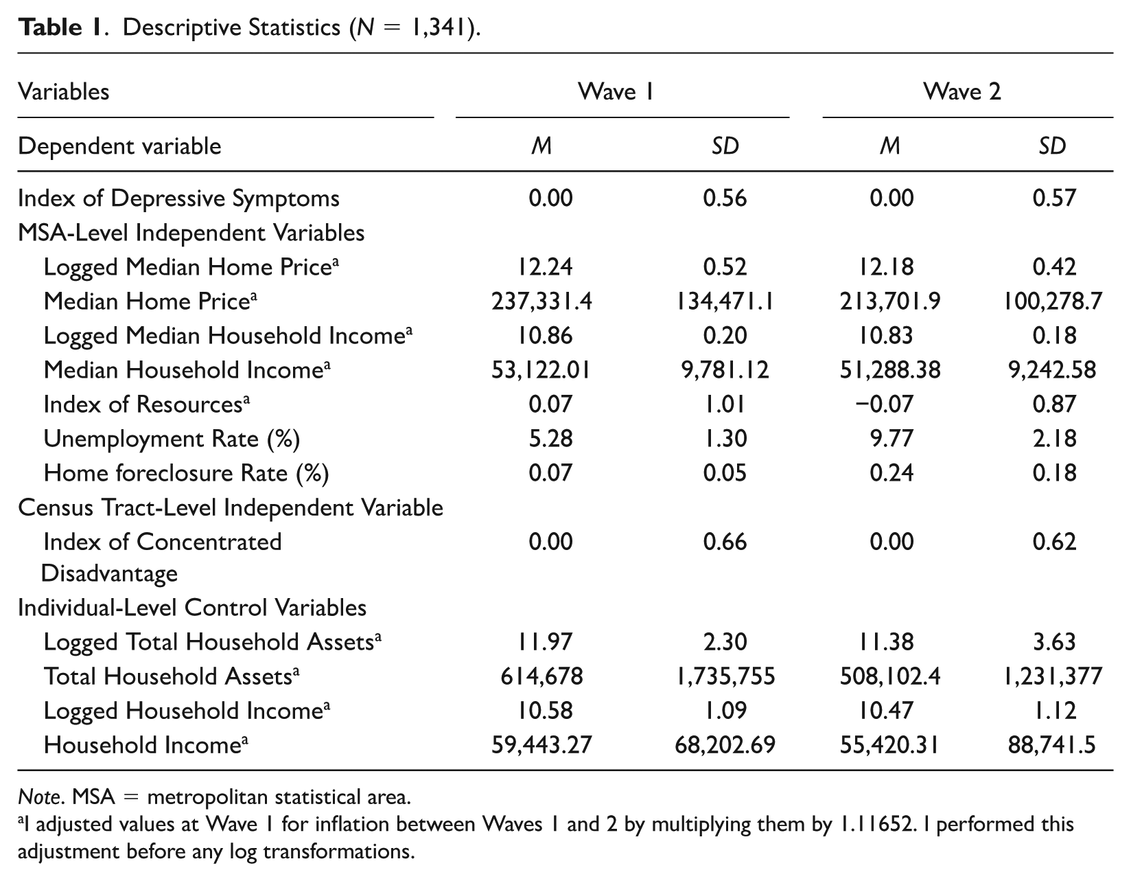
Note. MSA = metropolitan statistical area.

I adjusted values at Wave 1 for inflation between Waves 1 and 2 by multiplying them by 1.11652. I performed this adjustment before any log transformations.

Models 1 and 2 of Table 2 show that when the index of MSA-level resources is included along with the index of census tract-level concentrated disadvantage, MSA-level resources are significantly associated with fewer depressive symptoms (Model 1: coeff.: −0.222, p < .01; Model 2: coeff.: −0.214, p < .01), whereas the coefficient of census tract-level concentrated disadvantage does not reach statistical significance.

Table 2.

Fixed-Effects Linear Regression Analyses of the Impact of an Index of City-Level Resources on Depressive Symptoms.

Variables	Model 1	Model 2	Model 3	Model 4
Index of MSA-Level Resources	−0.222** (0.073)	−0.214** (0.073)	−0.210** (0.073)	−0.203** (0.072)
Index of Census Tract-Level Concentrated Disadvantage	−0.010 (0.060)	−0.016 (0.059)	−0.002 (0.060)	−0.007 (0.059)
Index of MSA-Level Resources × Index of Census Tract-Level Concentrated Disadvantage			−0.067* (0.033)	−0.064(0.034)
Logged Total Household Assets		−0.006(0.006)		−0.006(0.007)
Logged Household Income		−0.006(0.013)		−0.005(0.012)
Constant	0.010(0.007)	0.146(0.139)	0.007(0.006)	0.129(0.141)
Observations	2,681	2,681	2,681	2,681
df(Model/Residual)	2/57	4/57	3/57	5/57
R ²	.019	.021	.022	.024
Number of Respondents	1,341	1,341	1,341	1,341

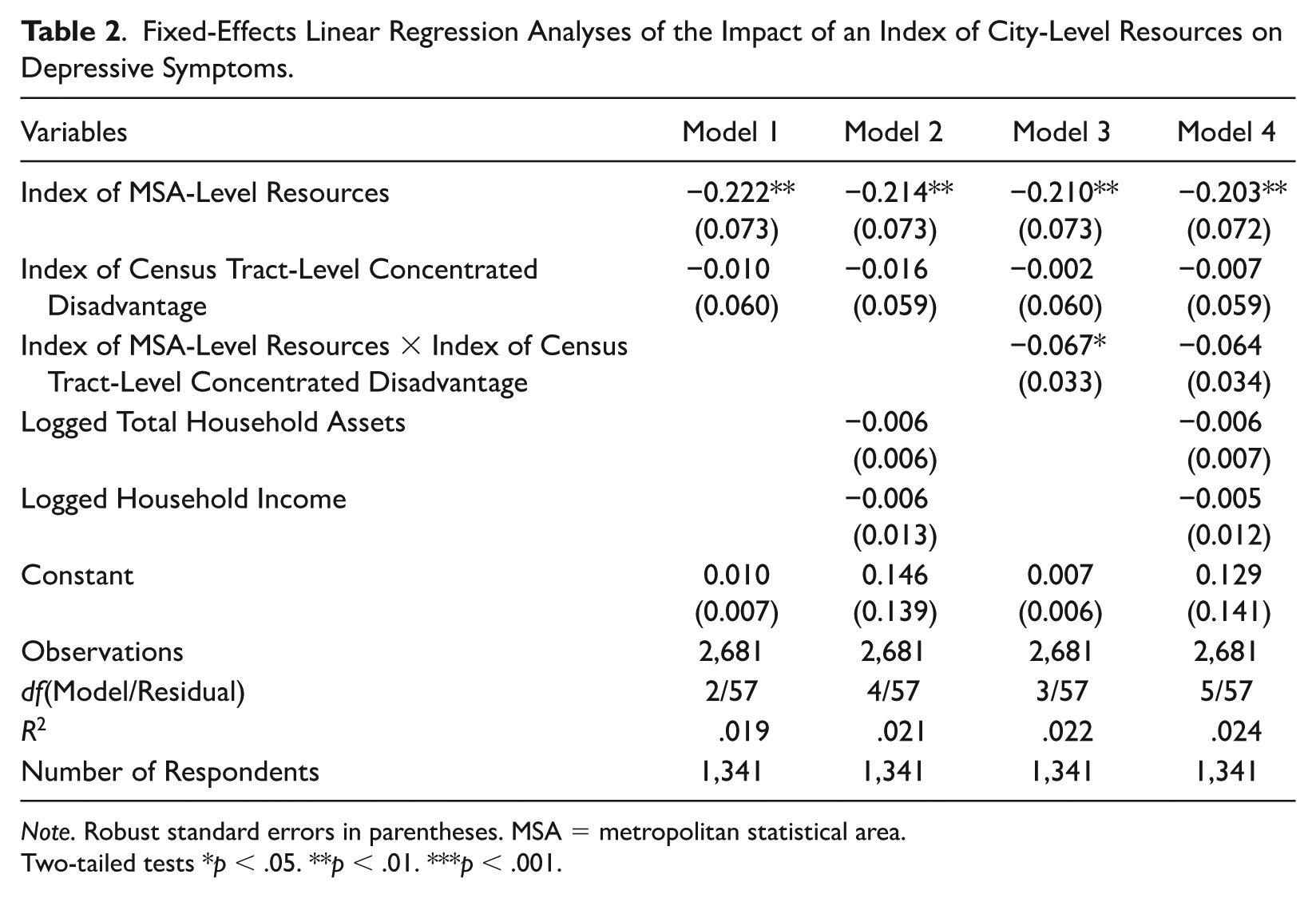
Note. Robust standard errors in parentheses. MSA = metropolitan statistical area.

Two-tailed tests *p < .05. **p < .01. ***p < .001.

Model 3 of Table 2 adds to Model 1 an interaction term between the index of MSA-level resources and the index of census tract-level concentrated disadvantage. This model shows that when census tract-level concentrated disadvantage remains constant over the two waves, an increase in MSA-level resources implies significantly fewer depressive symptoms (coeff.: −0.210, p < 0.01). When MSA-level resources stay constant over the two waves, a change in census tract-level concentrated disadvantage does not result in a statistically significant change in depressive symptoms. The interaction term between MSA-level resources and census tract-level concentrated disadvantage achieves statistical significance (coeff.: −0.067, p < 0.05). This implies that when census tract-level concentrated disadvantage rises, increases in resources at the MSA level become more important for reducing depressive symptoms. This is likely because amid an economic recession, city resources channeled into declining neighborhoods aid the preservation of streets (Allen 2013), the repurchasing and upkeep of vacated buildings, and the reduction of foreclosures (Baumer et al. 2012), all of which help preserve neighborhoods’ quality, order, and safety (Leonard and Murdoch 2009). As such, greater extents of city-level resources become especially valuable for supporting residents’ mental health within neighborhoods experiencing intensified deprivation and need for investment and improvement.

The magnitude of this interaction coefficient suggests that when census tract-level concentrated disadvantage rises (or declines) by 1 SD, the association between rising city-level resources and decreasing depressive symptoms increases (or decreases) by about 20 percent. While this effect is of modest size, it is not negligible. The modest size of this moderation effect is expected given scholarship that argues that contextual effects are usually of lower magnitude than those of features of respondents themselves (see Oberwittler 2004; Pickett and Pearl 2001; Stjärne, de Leon, and Hallqvist 2004).

Model 4 of Table 2 adds to Model 3 individual-level logged total household assets and logged household income. It is notable that the magnitude of the coefficient for the interaction between city-level resources and census tract-level concentrated disadvantage slightly decreases (coeff.: −0.064), reducing it to insignificance.

Figure 1 graphically displays the fixed-effects statistically significant interaction within Model 3 of Table 2. On the x-axis is the index of MSA-level resources, whereas on the y-axis is the index of depressive symptoms. The three lines denote 1 SD below the mean, the mean, and 1 SD above the mean in census tract-level concentrated disadvantage. This figure shows that the negative slope between MSA-level resources and depressive symptoms is steeper for those undergoing greater census tract-level concentrated disadvantage: there is an approximate 20 percent increase (or decrease) in steepness of slope between the line denoting the mean in concentrated disadvantage and the line representing 1 SD above (or below) the mean in concentrated disadvantage.

Figure 1.

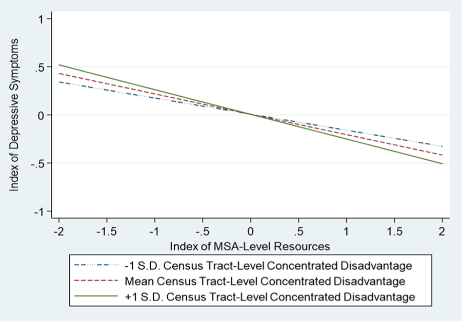
Graph displaying how the index of depressive symptoms is affected by the interaction between an index of MSA-level resources and census tract-level concentrated disadvantage (based on Model 3).

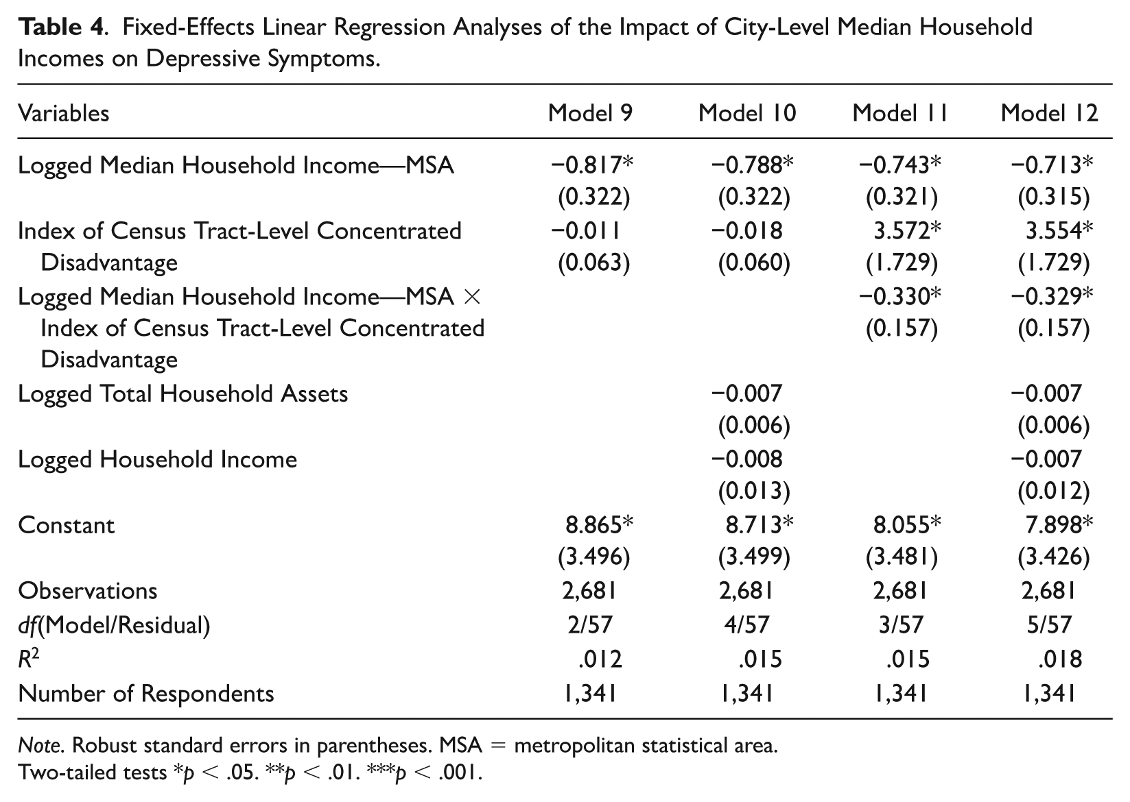
Tables 3 and 4 reveal that my findings within Table 2 concerning the interaction between city-level resources and census tract-level concentrated disadvantage are driven primarily by MSA-level median household incomes. Models 7 and 8 in Table 3 show that the interaction term between logged MSA-level median home prices and census tract-level concentrated disadvantage is statistically insignificant. Models 11 and 12 in Table 4 reveal that logged MSA-level median household incomes interact with census tract-level concentrated disadvantage in much the same way as the index of MSA-level resources, except that this interaction term maintains statistical significance when I further control for individual-level total household assets and household incomes (Model 11: coeff.: −0.330, p < 0.05; Model 12: coeff.: −0.329, p < 0.05). The magnitude of the interaction coefficient within Model 12 suggests that a 1 SD increase (or decrease) in census tract-level concentrated disadvantage implies an approximate 30 percent rise (or decline) in the extent to which increasing logged MSA-level median household incomes are associated with fewer depressive symptoms.

Table 3.

Fixed-Effects Linear Regression Analyses of the Impact of City-Level Median Home Prices on Depressive Symptoms.

Variables	Model 5	Model 6	Model 7	Model 8
Logged Median Home Price—MSA	−0.368** (0.132)	−0.353** (0.130)	−0.365** (0.128)	−0.352** (0.126)
Index of Census Tract-Level Concentrated Disadvantage	0.017(0.058)	0.011(0.056)	1.673(0.943)	1.570(0.979)
Logged Median Home Price—MSA × Index of Census Tract-Level Concentrated Disadvantage			−0.134(0.074)	−0.127(0.077)
Logged Total Household Assets		−0.006(0.006)		−0.005(0.007)
Logged Household Income		−0.006(0.013)		−0.004(0.013)
Constant	4.508** (1.615)	4.457** (1.593)	4.468** (1.564)	4.413** (1.542)
Observations	2,681	2,681	2,681	2,681
df(Model/Residual)	2/57	4/57	3/57	5/57
R ²	.016	.018	.020	.021
Number of Respondents	1,341	1,341	1,341	1,341

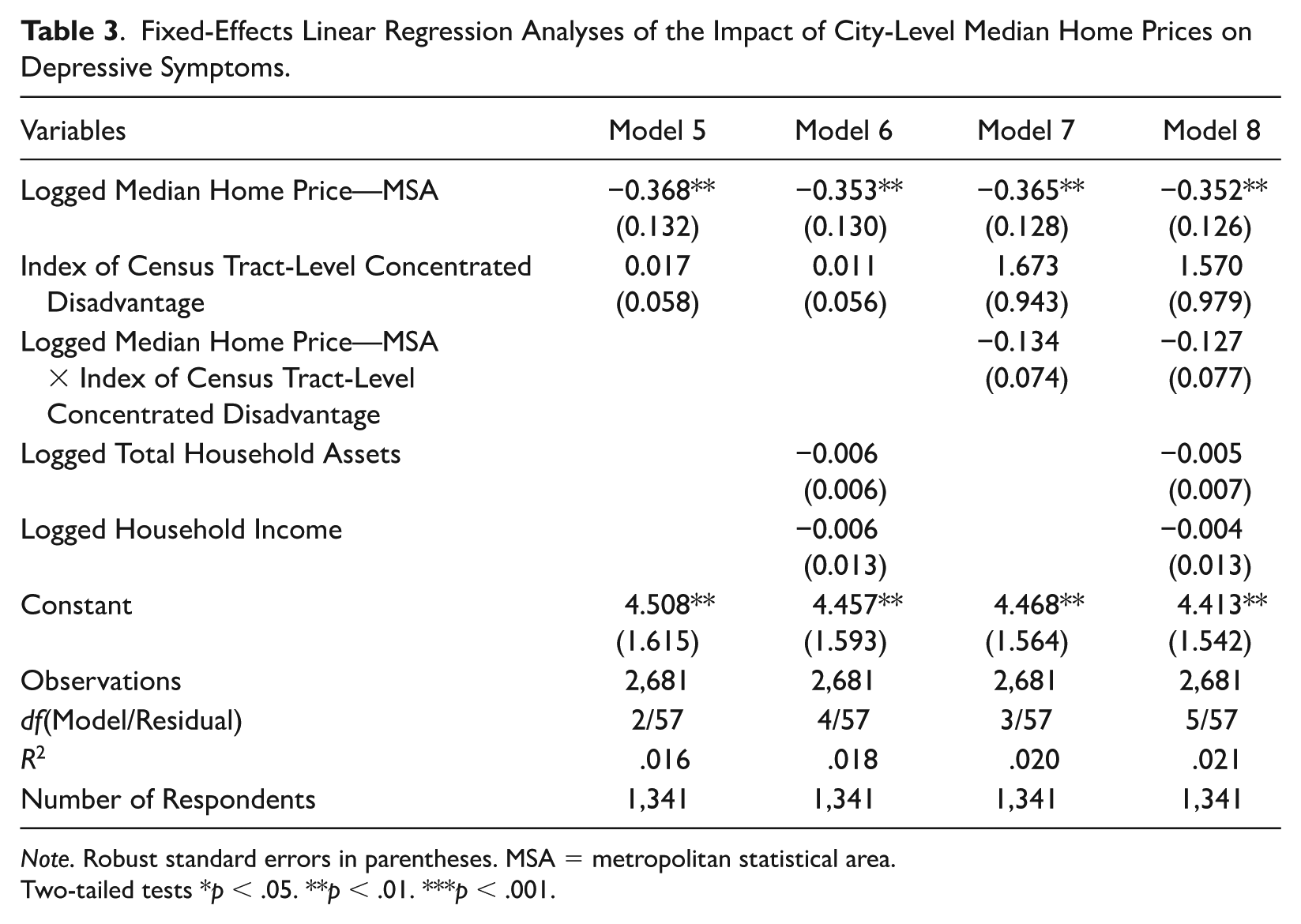
Note. Robust standard errors in parentheses. MSA = metropolitan statistical area.

Two-tailed tests *p < .05. **p < .01. ***p < .001.

Table 4.

Fixed-Effects Linear Regression Analyses of the Impact of City-Level Median Household Incomes on Depressive Symptoms.

Variables	Model 9	Model 10	Model 11	Model 12
Logged Median Household Income—MSA	−0.817* (0.322)	−0.788* (0.322)	−0.743* (0.321)	−0.713* (0.315)
Index of Census Tract-Level Concentrated Disadvantage	−0.011(0.063)	−0.018(0.060)	3.572* (1.729)	3.554* (1.729)
Logged Median Household Income—MSA × Index of Census Tract-Level Concentrated Disadvantage			−0.330* (0.157)	−0.329* (0.157)
Logged Total Household Assets		−0.007(0.006)		−0.007(0.006)
Logged Household Income		−0.008(0.013)		−0.007(0.012)
Constant	8.865* (3.496)	8.713* (3.499)	8.055* (3.481)	7.898* (3.426)
Observations	2,681	2,681	2,681	2,681
df(Model/Residual)	2/57	4/57	3/57	5/57
R ²	.012	.015	.015	.018
Number of Respondents	1,341	1,341	1,341	1,341

Note. Robust standard errors in parentheses. MSA = metropolitan statistical area.

Two-tailed tests *p < .05. **p < .01. ***p < .001.

Figure 2 graphically presents the fixed-effects statistically significant interaction within Model 12 of Table 4. While the x-axis represents logged MSA-level median household incomes, the y-axis denotes the index of depressive symptoms. As in Figure 1, the three lines represent 1 SD below the mean, the mean, and 1 SD above the mean in census tract-level concentrated disadvantage. This figure displays an approximate 30 percent rise (or decline) in the steepness of the negative slope between logged MSA-level median household incomes and depressive symptoms between the line representing the mean in concentrated disadvantage and the line denoting 1 SD above (or below) this mean. This figure shows how increases in city-level median household incomes become even more valuable for reducing residents’ depressive symptoms within neighborhoods undergoing increased disadvantage and need for city-level support and investment.

Figure 2.

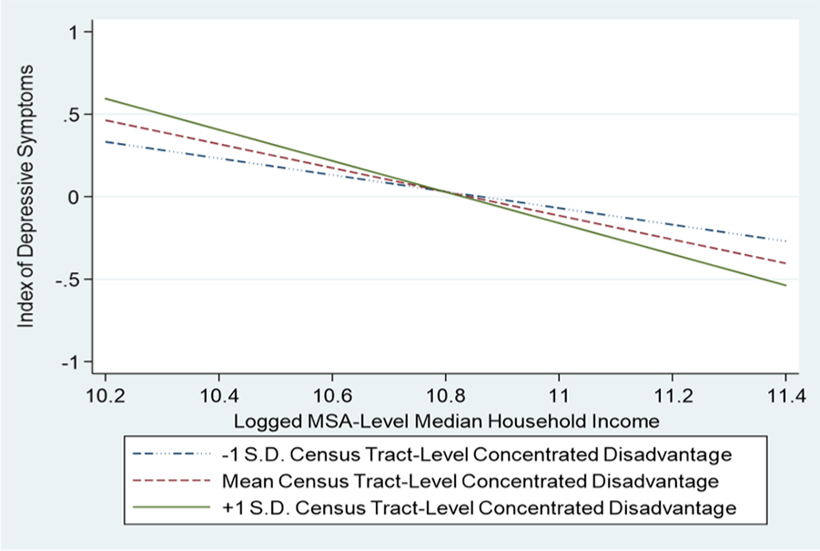
Graph displaying how the index of depressive symptoms is affected by the interaction between logged MSA-level median household incomes and census tract-level concentrated disadvantage (based on Model 12).

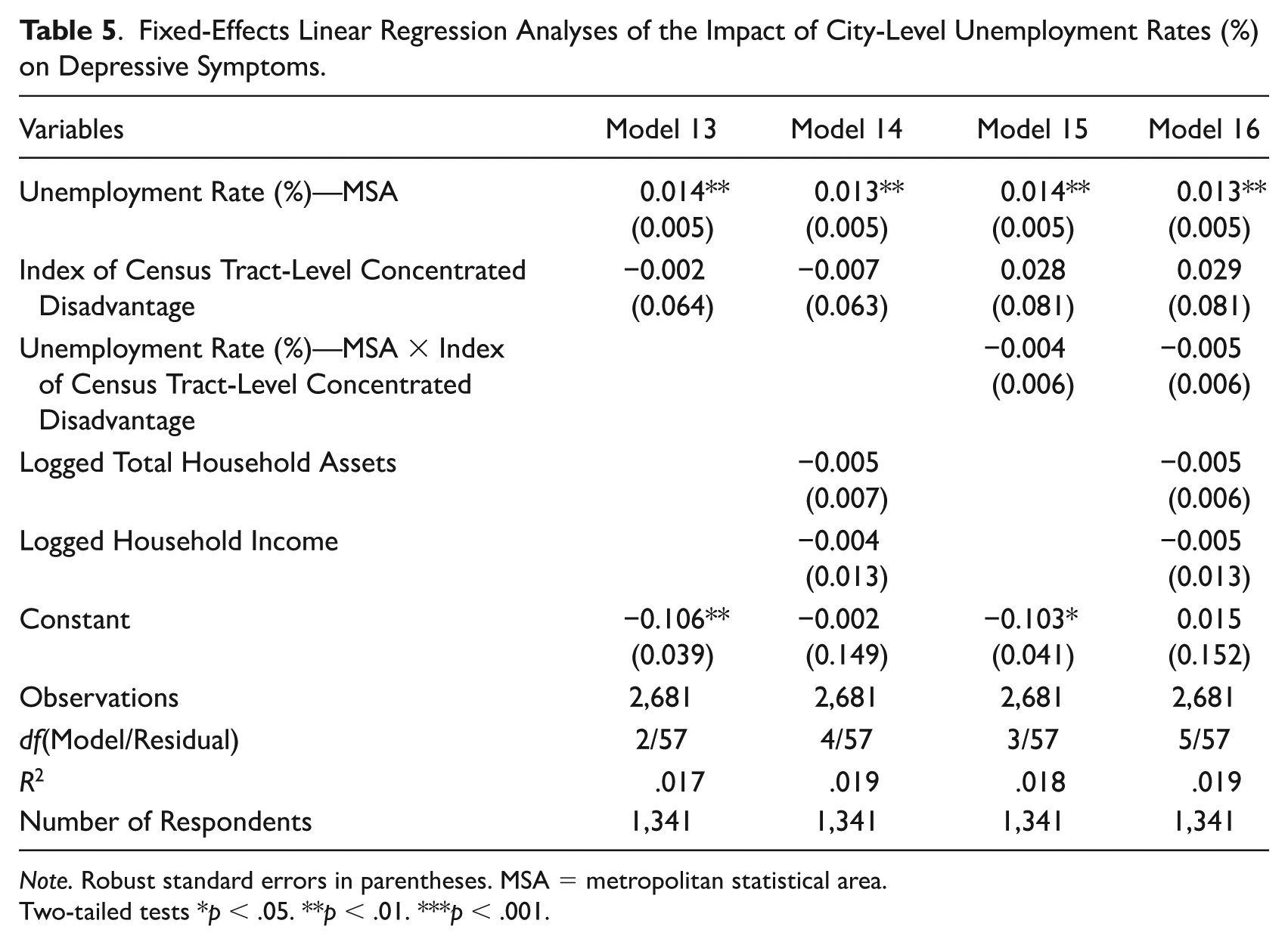
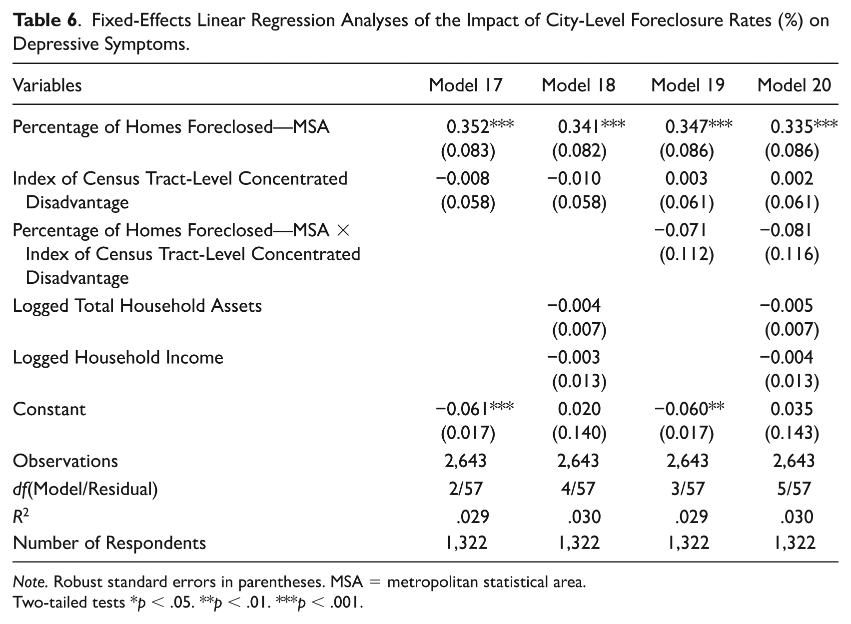
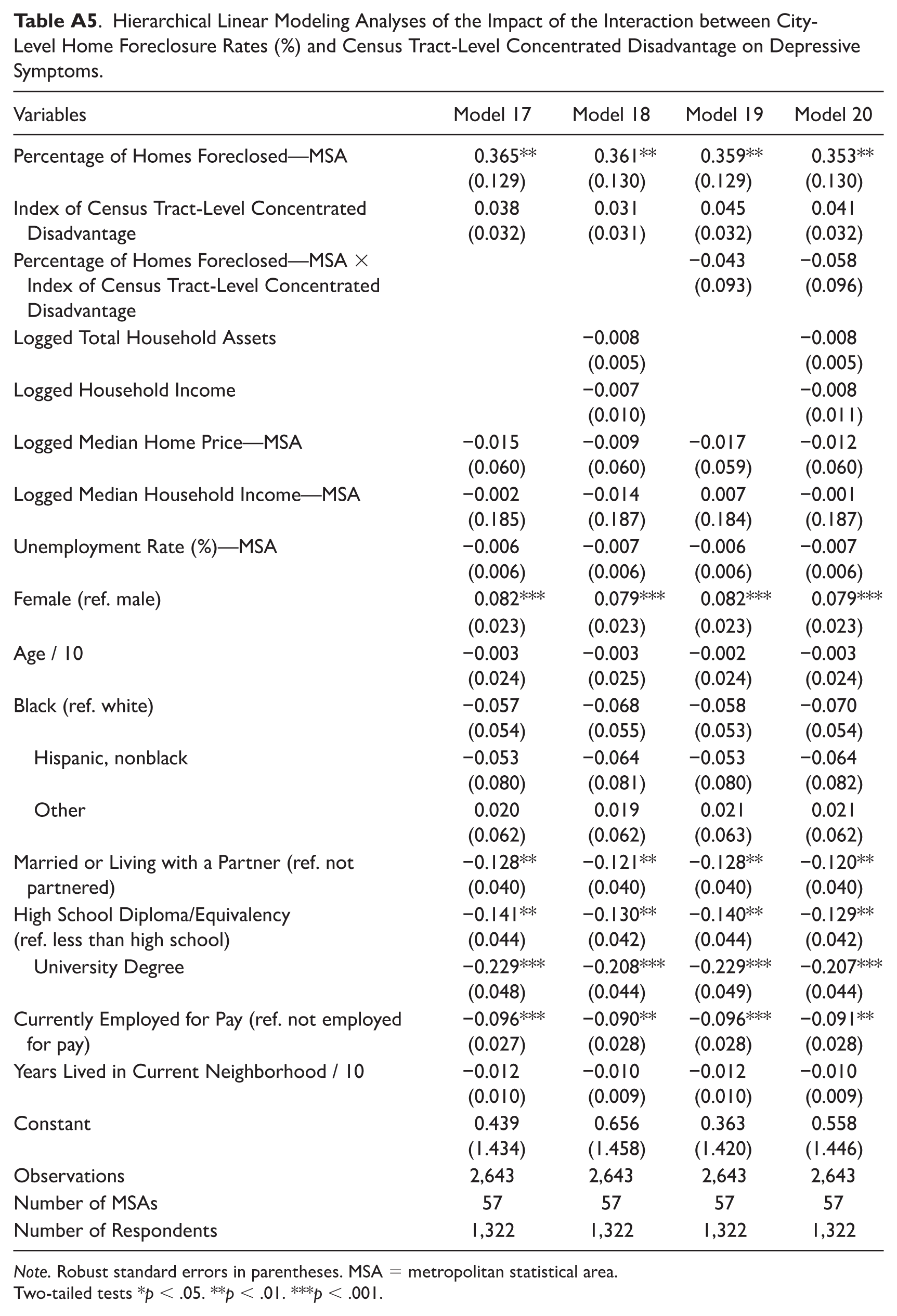
Tables 5 and 6 show that MSA-level unemployment rates (%) and home foreclosure rates (%) are significantly associated with increased depressive symptoms. However, neither of these two MSA-level variables significantly interact with census tract-level concentrated disadvantage.

Table 5.

Fixed-Effects Linear Regression Analyses of the Impact of City-Level Unemployment Rates (%) on Depressive Symptoms.

Variables	Model 13	Model 14	Model 15	Model 16
Unemployment Rate (%)—MSA	0.014** (0.005)	0.013** (0.005)	0.014** (0.005)	0.013** (0.005)
Index of Census Tract-Level Concentrated Disadvantage	−0.002(0.064)	−0.007(0.063)	0.028(0.081)	0.029(0.081)
Unemployment Rate (%)—MSA × Index of Census Tract-Level Concentrated Disadvantage			−0.004(0.006)	−0.005(0.006)
Logged Total Household Assets		−0.005(0.007)		−0.005(0.006)
Logged Household Income		−0.004(0.013)		−0.005(0.013)
Constant	−0.106** (0.039)	−0.002(0.149)	−0.103* (0.041)	0.015(0.152)
Observations	2,681	2,681	2,681	2,681
df(Model/Residual)	2/57	4/57	3/57	5/57
R ²	.017	.019	.018	.019
Number of Respondents	1,341	1,341	1,341	1,341

Note. Robust standard errors in parentheses. MSA = metropolitan statistical area.

Two-tailed tests *p < .05. **p < .01. ***p < .001.

Table 6.

Fixed-Effects Linear Regression Analyses of the Impact of City-Level Foreclosure Rates (%) on Depressive Symptoms.

Variables	Model 17	Model 18	Model 19	Model 20
Percentage of Homes Foreclosed—MSA	0.352*** (0.083)	0.341*** (0.082)	0.347*** (0.086)	0.335*** (0.086)
Index of Census Tract-Level Concentrated Disadvantage	−0.008(0.058)	−0.010(0.058)	0.003(0.061)	0.002(0.061)
Percentage of Homes Foreclosed—MSA × Index of Census Tract-Level Concentrated Disadvantage			−0.071(0.112)	−0.081(0.116)
Logged Total Household Assets		−0.004(0.007)		−0.005(0.007)
Logged Household Income		−0.003(0.013)		−0.004(0.013)
Constant	−0.061*** (0.017)	0.020(0.140)	−0.060** (0.017)	0.035(0.143)
Observations	2,643	2,643	2,643	2,643
df(Model/Residual)	2/57	4/57	3/57	5/57
R ²	.029	.030	.029	.030
Number of Respondents	1,322	1,322	1,322	1,322

Note. Robust standard errors in parentheses. MSA = metropolitan statistical area.

Two-tailed tests *p < .05. **p < .01. ***p < .001.

Robustness Check

The results of my HLM analysis robustness check (presented in the appendix) correspond with my central fixed-effects linear regression results. Model 3 within Table A1, in which individual-level total household assets and household incomes are not controlled, shows that rising census tract-level concentrated disadvantage significantly accentuates how increases in the index of MSA-level resources reduce depressive symptoms. When individual-level total household assets and household incomes are further controlled in Model 4, a slight increase in the standard error of this interaction term reduces it to insignificance. The corresponding interaction term coefficients for logged MSA-level median home prices (see Table A2) and logged MSA-level median household incomes (see Table A3) are in the same direction as in the main analyses but neither reaches statistical significance, with and without further control for individual-level total household assets and household incomes. As such, findings for the interaction between logged MSA-level median household incomes and census tract-level concentrated disadvantage were weaker within the HLM robustness check than within the main analyses. As in the main analyses, the interaction term coefficients for MSA-level unemployment rates and home foreclosure rates were statistically insignificant. This concurrence between the main fixed-effects linear regression results and the HLM results supports the robustness of this study’s findings.

Discussion

I found that declining resources at the city level interact with increasing disadvantage at the neighborhood level in impacting older residents’ depressive symptoms. My results within Table 2 further show that when neighborhood-level concentrated disadvantage stays constant, rises in city-level resources decrease depressive symptoms among older persons. On the contrary, when resources at the city level stay constant, changes in neighborhood-level concentrated disadvantage do not significantly cause changes in older residents’ depressive symptoms.

My main finding is that when neighborhood-level concentrated disadvantage increases, rising city-level resources more potently decrease depressive symptoms. My HLM analyses produced the same main result and thus support the robustness of this finding. Table 2 reveals that when individual-level household income and total household assets are controlled, the magnitude of this interaction term coefficient is slightly reduced and becomes statistically insignificant. This suggests that this moderation effect operates through detrimental changes in features of contexts and, to some extent, through personal financial declines.

During economic recessions, fewer city resources imply less provision of services to needy neighborhoods, including the maintenance of streets (Allen 2013), foreclosure mitigation, and the maintenance and repurchasing of vacated and abandoned buildings (Baumer et al. 2012). More home foreclosures and abandoned buildings create neighborhood-level externalities that reduce home values while raising levels of disorder and criminal activity (Leonard and Murdoch 2009). Greater extents of disorder and crime lead to stress and fear, which impact mental health. This suggests that fewer city funds to repair and improve neighborhoods are especially damaging to mental health within neighborhoods undergoing increased disadvantage and need. In addition, a decline in the value of one’s primary residence implies loss of a large portion of one’s accumulated assets (see De Nardi et al. 2012). Declining city resources also entails less stimulus spending that can improve labor market conditions and support older Americans’ household incomes (see Dethier and Morrill 2012; Miller and Hokenstad 2014).

There are numerous reasons why these effects might particularly impact older residents. In general, neighborhood factors might more potently affect older adults due to their greater spatial confinement, which could be caused by retirement, functional health problems, and other later-life transitions and circumstances (Choi et al. 2015; Glass and Balfour 2003; Krantz-Kent and Stewart 2007). This higher spatial confinement leads older persons to be more dependent for their health and happiness on their communities’ infrastructure, institutions, amenities, businesses, services, and networks of supportive relationships (Choi et al. 2015), which decline within urban neighborhoods facing rising socioeconomic challenges (Chernick, Langley, and Reschovsky 2011; Kazembe and Nickanor 2017; Leventhal and Brooks-Gunn 2003; McDaniel, Gazso, and Um 2013; Modrek et al. 2013; Peck 2012; Tendler 1982; Weffer et al. 2014). These downturns include detriments to the public transit systems upon which older persons depend because of diminished mobility (Rosenbloom 2009; Su and Bell 2009) and to the senior centers and other community social amenities that help older persons remain socially engaged (Aneshensel, Harig, and Wight 2016). In addition, older adults show high extents of anxiety concerning violence and other criminal activity (Fried and Barron 2005; Piro, Noss, and Claussen 2006). Confinement to one’s immediate neighborhood further accentuates older persons’ susceptibility to and fear of the rising rates of crime and disorder commonplace within worsening urban environments (Fried and Barron 2005; Leonard and Murdoch 2009; Lerman and Zhang 2012; Piro et al. 2006). Circumstances for older persons worsen when there are fewer city resources to channel into declining communities to halt and reverse such downturns.

In addition, the Great Recession compromised the retirement security of many older Americans, obliging many to extend their paid employment within a workforce that is disadvantageous for older employees (Munnell and Rutledge 2013). Fewer city resources for neighborhoods in need suggest less stimulus spending that can create good employment opportunities for older persons and that can fund retraining programs that help equip older workers with the skills required in the present-day workforce.

This discussion of how city- and neighborhood-level changes interact in affecting older residents’ depressive symptoms fits the compound disadvantage model’s claim that separate sources of similar types of disadvantages combine in a multiplicative manner as they affect physical and mental health (Wheaton and Clarke 2003). I have identified the multiplicative effects of negative socioeconomic changes at the city and neighborhood levels.

Of the various city-level conditions considered, those pertaining most directly to tax revenues and resource availability showed the strongest interactive effects with census tract-level concentrated disadvantage. MSA-level median home prices (see Chatterjee and Eyigungor 2015; Diamond 2017; Kahn 2017; Lutz 2008) and median household incomes (see Brasier et al. 2011; Chatterjee and Eyigungor 2015; Jha 2017; Maher and Deller 2011) are both important determinants of cities’ tax revenues, and thus of the availability of city resources for neighborhoods in need, as well as for spending on citywide public goods and services. Tables 3 and 4 show that the significant interaction between MSA-level resources and census tract-level concentrated disadvantage is based mostly on MSA-level median household incomes. While the interaction term between logged MSA-level median home prices and census tract-level concentrated disadvantage is statistically insignificant, Model 12 from Table 4 reveals the interaction between logged MSA-level median household incomes and census tract-level concentrated disadvantage to maintain statistical significance even after control for individual-level household income and total household assets. MSA-level unemployment rates and extents of homes foreclosed do not significantly interact with census tract-level concentrated disadvantage, possibly because they are less direct determinants of the resources available within the larger city than home prices and household incomes.

Limitations and Paths for Future Research

Future research should replicate this study with measures of actual policy decisions that channel resources at the city level into city neighborhoods. While it is broadly accurate that cities showing less declines in resources will be more likely to meet the increased needs of their declining neighborhoods, cities undergoing similar economic declines through the Great Recession are likely to have differed in their policy responses, including austerity measures and stimulus spending. This implies different extents of unmet needs within their declining neighborhoods.

In this study, I focus on depressive symptoms, which are a measure of mental health that can vary in the short term as one’s life situation changes, including economic changes within one’s city and neighborhood (Burgard and Kalousova 2015). As such, they are an effective dependent variable for this study focused on the short-term impacts of economic downturns. An interesting follow-up project might repeat this analysis with a longer span of time to study effects on measures of physical health, which might take more than five years to substantially change. Burgard and Kalousova (2015) argued that studies of different health outcomes are associated with different appropriate spans of time. Studying how contextual economic changes impact measures of physical health is especially valuable within older samples because health declines accompany the process of aging.

Another fruitful path for future research is to replicate this study with a younger sample. Because of the biological vulnerabilities and cognitive declines that accompany the aging process, older persons might be more dependent than younger persons on the services, social programs, amenities, institutions, and infrastructure within their cities and neighborhoods. Therefore, city-level resources and neighborhood-level need might less potently affect the depressive symptoms of younger adults. On the contrary, younger adults might be more concerned with their paid work trajectories and providing for their families. If declines in cities’ resources cause less stimulus spending and creation of job opportunities within city neighborhoods, many younger adults might experience depressive symptoms as they struggle with underemployment and unemployment.

Footnotes

Appendix

Table A5.

Hierarchical Linear Modeling Analyses of the Impact of the Interaction between City-Level Home Foreclosure Rates (%) and Census Tract-Level Concentrated Disadvantage on Depressive Symptoms.

Variables	Model 17	Model 18	Model 19	Model 20
Percentage of Homes Foreclosed—MSA	0.365** (0.129)	0.361** (0.130)	0.359** (0.129)	0.353** (0.130)
Index of Census Tract-Level Concentrated Disadvantage	0.038 (0.032)	0.031 (0.031)	0.045 (0.032)	0.041 (0.032)
Percentage of Homes Foreclosed—MSA × Index of Census Tract-Level Concentrated Disadvantage			−0.043(0.093)	−0.058(0.096)
Logged Total Household Assets		−0.008(0.005)		−0.008(0.005)
Logged Household Income		−0.007(0.010)		−0.008(0.011)
Logged Median Home Price—MSA	−0.015(0.060)	−0.009(0.060)	−0.017(0.059)	−0.012(0.060)
Logged Median Household Income—MSA	−0.002(0.185)	−0.014(0.187)	0.007(0.184)	−0.001(0.187)
Unemployment Rate (%)—MSA	−0.006(0.006)	−0.007(0.006)	−0.006(0.006)	−0.007(0.006)
Female (ref. male)	0.082***	0.079***	0.082***	0.079***
Female (ref. male)	(0.023)	(0.023)	(0.023)	(0.023)
Age / 10	−0.003(0.024)	−0.003(0.025)	−0.002(0.024)	−0.003(0.024)
Black (ref. white)	−0.057(0.054)	−0.068(0.055)	−0.058(0.053)	−0.070(0.054)
Hispanic, nonblack	−0.053(0.080)	−0.064(0.081)	−0.053(0.080)	−0.064(0.082)
Other	0.020(0.062)	0.019(0.062)	0.021(0.063)	0.021(0.062)
Married or Living with a Partner (ref. not partnered)	−0.128** (0.040)	−0.121** (0.040)	−0.128** (0.040)	−0.120** (0.040)
High School Diploma/Equivalency(ref. less than high school)	−0.141** (0.044)	−0.130** (0.042)	−0.140** (0.044)	−0.129** (0.042)
University Degree	−0.229*** (0.048)	−0.208*** (0.044)	−0.229*** (0.049)	−0.207*** (0.044)
Currently Employed for Pay (ref. not employed for pay)	−0.096*** (0.027)	−0.090** (0.028)	−0.096*** (0.028)	−0.091** (0.028)
Years Lived in Current Neighborhood / 10	−0.012(0.010)	−0.010(0.009)	−0.012(0.010)	−0.010(0.009)
Constant	0.439(1.434)	0.656(1.458)	0.363(1.420)	0.558(1.446)
Observations	2,643	2,643	2,643	2,643
Number of MSAs	57	57	57	57
Number of Respondents	1,322	1,322	1,322	1,322

Note. Robust standard errors in parentheses. MSA = metropolitan statistical area.

Two-tailed tests *p < .05. **p < .01. ***p < .001.

Acknowledgements

Data were made available by the Interuniversity Consortium for Political and Social Research, Ann Arbor, MI, USA. Neither the collector of the original data nor the Consortium bears any responsibility for the analyses or interpretations presented here. I acknowledge the extensive help I received from Professor Markus Schafer, Professor Geoffrey Wodtke, and Professor Brent Berry.

Funding

The author(s) disclosed receipt of the following financial support for the research, authorship, and/or publication of this article: This work was supported by the Canadian Social Sciences and Humanities Research Council (Insight Development Grant No. 231615 and Doctoral Fellowship) and the Ontario Ministry of Research and Innovation Early Researcher Award. This work was also supported by the Ontario Student Assistance Program. Further support was provided by the Faculty of Humanities, Education and Social Sciences, University of Luxembourg, 2020 Research Block Grant Allocation Scheme–Merit Based Funding Scheme: Incentive B. These funding sources had no involvement in study design; in the collection, analysis, and interpretation of data; in the writing of the article; and in the decision to submit it for publication.

References

Acevedo-Garcia

Dolores

Lochner

Kimberly A.

Osypuk

Theresa L.

Subramanian

S. V.

2003. “Future Directions in Residential Segregation and Health Research: A Multilevel Approach.” American Journal of Public Health 93:215–21.

Ackerman

Robert A.

Fries

Gerhard

Windle

Richard A.

2012. “Changes in US Family Finances from 2007 to 2010: Evidence from the Survey of Consumer Finances.” Federal Reserve Bulletin 1:1–80.

Allen

Ryan

. 2013. “The Distribution and Evolution of Physical Neighborhood Problems during the Great Recession.” City and Community 12:260–79.

Aneshensel

Carol S.

2010. “Neighborhood as a Social Context of the Stress Process.” Pp. 35–52 in Advances in the Conceptualization of the Stress Process: Essays in Honor of Leonard I. Pearlin, edited by Avison

W. R.

Aneshensel

C. S.

Schieman

Wheaton

New York: Springer.

Aneshensel

Carol S.

Harig

Frederick

Wight

Richard G.

2016. “Chapter 15: Aging, Neighborhoods, and the Built Environment.” Pp. 315–35 in Handbook of Aging and the Social Sciences, 8th ed., edited by George

L. K.

Ferraro

K. F.

San Diego, CA: Academic Press.

Aneshensel

Carol S.

Michelle J.

Chodosh

Joshua

Wight

Richard G.

2011. “The Urban Neighborhood and Cognitive Functioning in Late Middle Age.” Journal of Health and Social Behavior 52:163–79.

Arias

Maria A.

Gascon

Charles S.

Rapach

David E.

2016. “Metro Business Cycles.” Working Paper Series. Research Division, Federal Reserve Bank of St. Louis. Retrieved December 1, 2020 (https://files.stlouisfed.org/files/htdocs/wp/2014/2014-046.pdf).

ATTOM Data Solutions. N.d. Retrieved November 16, 2017 (https://www.attomdata/com).

Austen

Siobhan

Ong

Rachel

. 2009. “The Employment Transitions of Mid-Life Women: Health and Care Effects.” Ageing & Society 30:207–27.

10.

Baumer

Eric P.

Wolff

Kevin T.

Arnio

Ashley N.

2012. “A Multicity Neighborhood Analysis of Foreclosure and Crime.” Social Science Quarterly 93:577–601.

11.

Blazer

Dan G.

2003. “Depression in Late Life: Review and Commentary.” The Journals of Gerontology, Series A: Biological Sciences & Medical Sciences 58:249–65.

12.

Boen

Courtney

Yang

Yang Claire

. 2016. “The Physiological Impacts of Wealth Shocks in Late Life: Evidence from the Great Recession.” Social Science and Medicine 150:221–30.

13.

Brasier

Kathryn J.

Filteau

Matthew R.

McLaughlin

Diane K.

Jacquet

Jeffrey

Stedman

Richard C.

Kelsey

Timothy W.

Goetz

Stephan J.

2011. “Residents’ Perceptions of Community and Environmental Impacts from Development of Natural Gas in the Marcellus Shale: A Comparison of Pennsylvania and New York Cases.” Journal of Rural Social Sciences 26:32–61.

14.

Brown

Robert L.

2011. “Economic Security in an Aging Canadian Population.” Canadian Journal on Aging 30:391–99.

15.

Burgard

Sarah A.

Kalousova

Lucie

. 2015. “Effects of the Great Recession: Health and Well-Being.” Annual Review of Sociology 41:181–201.

16.

Burgard

Sarah A.

Seefeldt

Kristin S.

Zelner

Sarah

. 2012. “Housing Instability and Health: Findings from the Michigan Recession and Recovery Study.” Social Science & Medicine 75(12):2215–24.

17.

Bursik

Robert J.

1988. “Social Disorganization and Theories of Crime and Delinquency: Problems and Prospects.” Criminology 26:519–52.

18.

Cagney

Kathleen A.

Browning

Christopher R.

Iveniuk

James

English

Ned

. 2014. “The Onset of Depression during the Great Recession: Foreclosure and Older Adult Mental Health.” American Journal of Public Health 104:498–505.

19.

Chatterjee

Satyajit

Eyigungor

Burcu

. 2015. “A Quantitative Analysis of the U.S. Housing and Mortgage Markets and the Foreclosure Crisis.” Review of Economic Dynamics 18:165–84.

20.

Chernick

Howard

Langley

Adam

Reschovsky

Andrew

. 2011. “The Impact of the Great Recession and the Housing Crisis on the Financing of America’s Largest Cities.” Regional Science and Urban Economics 41:372–81.

21.

Choi

Namkee G.

Kim

Jinseok

DiNitto

Diana M.

Marti

C. Nathan

. 2015. “Perceived Social Cohesion, Frequency of Going out, and Depressive Symptoms in Older Adults: Examination of Longitudinal Relationships.” Gerontology and Geriatric Medicine 1:1–11. Published electronically November 26. doi:10.1177/2333721415615478.

22.

Cooke

Martin

. 2006. “Policy Changes and the Labour Force Participation of Older Workers: Evidence from Six Countries.” Canadian Journal on Aging 25:387–400.

23.

Cornwell

Benjamin

Laumann

Edward O.

Schumm

L. Philip

. 2008. “The Social Connectedness of Older Adults: A National Profile.” American Sociological Review 73:185–203.

24.

Cramm

Jane M.

van Dijk

Hanna M.

Nieboer

Anna P.

2013. “The Importance of Neighborhood Social Cohesion and Social Capital for the Well Being of Older Adults in the Community.” Gerontologist 53:142–50.

25.

David

Javier E.

2018. “Big Metropolitan Cities Are Seeing High Levels of Residential Segregation, Study Finds.” CNBC, May 24. Retrieved October 1, 2018 (https://www.cnbc.com/2018/05/23/metropolitan-housing-markets-like-new-york-chicago-are-highly-segregated.html).

26.

Davidson

Jacob

. 2014. “The 5 Cities That Have Recovered Most-and Least-From the Recession.” Money, July 30. Retrieved October 2, 2018 (https://money.com/5-cities-recession-recovery-most-least/).

27.

De Nardi

Mariacristina

French

Eric

Benson

David

. 2012. “Consumption and the Great Recession Economic Perspectives.” Economic Perspectives 36:1–16.

28.

Dethier

Jean-Jacques

Morrill

Curtis

. 2012. “The Great Recession and the Future of Cities.” World Bank Policy Research Working Paper No. 6256. World Bank, Washington, DC.

29.

Diamond

Rebecca

. 2017. “Housing Supply Elasticity and Rent Extraction by State and Local Governments.” American Economic Journal: Economic Policy 9:74–111.

30.

Diez Roux

Ana V.

2001. “Investigating Neighborhood and Area Effects on Health.” American Journal of Public Health 91(11):1783–89.

31.

Dill

Kathryn

. 2014. “Study Reveals U.S. Cities Most and Least Recovered since the Recession.” Forbes, June 23. Retrieved September 30, 2018 (https://www.forbes.com/sites/kathryndill/2014/06/23/study-reveals-u-s-cities-most-and-least-recovered-since-the-recession/#11fb9cfc1422).

32.

Downing

Janelle

. 2016. “The Health Effects of the Foreclosure Crisis and Unaffordable Housing: A Systematic Review and Explanation of Evidence.” Social Science and Medicine 162:88–96.

33.

Dragano

Nico

Bobak

Martin

Wege

Natalia

Peasey

Anne

Verde

Pablo E.

Kubinova

Ruzena

Weyers

Simone

Moebus

Susanne

Möhlenkamp

Stefan

Stang

Andreas

Erbel

Raimund

Jöckel

Karl-Heinz

Siegrist

Johannes

Pikha

Hynek

. 2007. “Neighbourhood Socioeconomic Status and Cardiovascular Risk Factors: A Multilevel Analysis of Nine Cities in the Czech Republic and Germany.” BMC Public Health 7:255.

34.

Estabrooks

Paul A.

Lee

Rebecca E.

Gyurcsik

Nancy C.

2003. “Resources for Physical Activity Participation: Does Availability and Accessibility Differ by Neighborhood Socioeconomic Status?” Annals of Behavioral Medicine 25:100–104.

35.

Feldman

Penny Hollander

Oberlink

Mia R.

2003. “The AdvantAge Initiative Developing Community Indicators to Promote the Health and Well-Being of Older People.” Family Community Health 26:268–74.

36.

Fiske

Amy

Wetherell

Julie L.

Gatz

Margaret

. 2009. “Depression in Older Adults.” Annual Review of Clinical Psychology 5:363–89.

37.

Florida

Richard

. 2015. “America’s Most Economically Segregated Cities.” Bloomberg: Citylab, February 23. Retrieved September 28, 2018 (https://www.citylab.com/life/2015/02/americas-most-economically-segregated-cities/385709/).

38.

Florida

Richard

. 2016. “Which U.S. Cities Suffer the Most During a Recession?” Bloomberg: Citylab, June 9. Retrieved September 26, 2018 (https://www.citylab.com/equity/2016/06/which-us-metros-suffer-the-most-during-a-recession/486263/).

39.

Florida

Richard

Mellander

Charlotta

. 2015. Segregated City: The Geography of Economic Segregation in America’s Metros. Toronto, ON, Canada: Martin Prosperity Institute.

40.

Fried

Linda

Barron

Jeremy

. 2005. “Older Adults: Guardians of our Cities.” Pp. 177–99 in Handbook of Urban Health: Populations, Methods, and Practice, edited by Galea

Vlahov

New York: Springer Science & Business Media.

41.

Galea

Sandro

Freudenberg

Nicholas

Vlahov

David

. 2005. “Cities and Population Health.” Social Science & Medicine 60:1017–33.

42.

Gilster

Megan E.

2014. “Neighborhood Stressors, Mastery, and Depressive Symptoms: Racial and Ethnic Differences in an Ecological Model of the Stress Process in Chicago.” Journal of Urban Health: Bulletin of the New York Academy of Medicine 91:690–706.

43.

Glass

Thomas A.

Balfour

Jennifer L.

2003. “Neighborhoods, Aging, and Functional Limitations.” Pp. 303–34 in Neighborhoods and Health, edited by Kawachi

Berkman

Oxford, England: Oxford University Press.

44.

Gray

Tom

Scardamalia

Robert

. 2014. “America’s Top Metros: Who’s Leading the Recovery, and Why.” Civic Report 89:1–41.

45.

Grusky

David B.

Western

Bruce

Wimer

Christopher

. 2011. “The Consequences of the Great Recession.” Pp. 3–20 in The Great Recession, edited by Grusky

David B.

Western

Bruce

Wimer

Christopher

. New York: Russell Sage Foundation.

46.

Hacker

Jacob S.

Huber

Gregory A.

Nichols

Austin

Rehm

Philipp

Craig

Stuart

. 2012. Economic Insecurity across the American States: New State Estimates from the Economic Security Index. Technical Report. New York: The Rockefeller Foundation.

47.

Hajat

Anjum

Kaufman

Jay S.

Rose

Kathryn M.

Siddiqi

Arjumand

Thomas

James C.

2010. “Do the Wealthy Have a Health Advantage? Cardiovascular Disease Risk Factors and Wealth.” Social Science & Medicine 71:1935–42.

48.

Hajat

Anjum

Kaufman

Jay S.

Rose

Kathryn M.

Siddiqi

Arjumand

Thomas

James C.

2011. “Long-Term Effects of Wealth on Mortality and Self-Rated Health Status.” American Journal of Epidemiology 173:192–200.

49.

Hawkley

Louise C.

Kocherginsky

Masha

Wong

Jaclyn

Kim

Juyeon

Cagney

Kathleen A.

2014. “Missing Data in Wave 2 of NSHAP: Prevalence, Predictors, and Recommended Treatment.” Journals of Gerontology, Series B: Psychological Sciences & Social Sciences 69:S38–50.

50.

Houle

Jason N.

2014. “Mental Health in the Foreclosure Crisis.” Social Science & Medicine 118(C):1–8.

51.

Houle

Jason N.

Light

Michael T.

2014. “The Home Foreclosure Crisis and Rising Suicide Rates, 2005 to 2010.” American Journal of Public Health 104:1073–79.

52.

Houle

Jason N.

Light

Michael T.

2017. “The Harder They Fall? Sex and Race/Ethnic Specific Suicide Rates in the U.S. Foreclosure Crisis.” Social Science & Medicine 180:114–24.

53.

Iceland

John

Weinberg

Daniel H.

Steinmetz

Erika

. 2002. Racial and Ethnic Residential Segregation in the United States: 1980-2000. U.S. Census Bureau, Series CENSR-3. Washington, DC: U.S. Government Printing Office.

54.

Jha

Nandan K.

2017. “Is There an Association between Fiscal Decentralization and Declining Role of State Governments in Highway Finance in the US?” Global Journal of Economics and Finance 1:1–14.

55.

Johnson

David

. 2005. “Two-Wave Panel Analysis: Comparing Statistical Methods for Studying the Effects of Transitions.” Journal of Marriage and Family 67:1061–75.

56.

Kahn

Matthew E.

2017. “Is Local Public Sector Rent Extraction Higher in Progressive Cities or High Amenity Cities? ” NBER Working Paper Series: Working Paper 23201. Retrieved December 1, 2020 (https://www.nber.org/system/files/working_papers/w23201/w23201.pdf).

57.

Kaplan

George A.

Everson

Susan A.

Lynch

John W.

2000. “The Contribution of Social and Behavioral Research to an Understanding of the Distribution of Disease: A Multilevel Approach.” Pp. 37–80 in Promoting Health: Intervention Strategies from Social and Behavioral Research, edited by Smedley

B. D.

Syme

S. L.

Washington, DC: National Academies Press.

58.

Katz

Charles M.

Wallace

Danielle

Hedberg

Eric C.

2013. “A Longitudinal Assessment of the Impact of Foreclosure on Neighborhood Crime.” Journal of Research in Crime and Delinquency 50:359–89.

59.

Kazembe

Lawrence N.

Nickanor

Ndeyapo M.

2017. “Spatial Modelling of the Relationship between Socio-Economic Disadvantage and Child Health in Namibia.” Spatial Demography 5:1–24.

60.

Kent

Alexander

Frohlich

Thomas C.

2015. “The 9 Most Segregated Cities in America.” Retrieved October 2, 2018 (https://www.huffingtonpost.com/entry/the-9-most-segregated-cities-in-america_us_55df53e9e4b0e7117ba92d7f).

61.

Kohli

Martin

Hank

Karsten

Kunemund

Harald

. 2009. “The Social Connectedness of Older Europeans: Patterns, Dynamics and Contexts.” Journal of European Social Policy 19:327–40.

62.

Krantz-Kent

Rachel

Stewart

Jay

. 2007. “How Do Older Americans Spend their Time?” Monthly Labor Review 130:8–26.

63.

LaVeist

Thomas A.

Wallace

John M.

Jr.

2000. “Health Risk and Inequitable Distribution of Liquor Stores in African American Neighborhood.” Social Science & Medicine 51:613–17.

64.

Lawton

M. P.

Nahemow

Lucille

. 1973. Ecology and the Aging Process. Washington, DC: American Psychological Association.

65.

Leonard

Tammy

Murdoch

James C.

2009. “The Neighborhood Effects of Foreclosure.” Journal of Geographical Systems 11:317–32.

66.

Lerman

Robert I.

Zhang

Sisi

. 2012. “Coping with the Great Recession: Disparate Impacts on Economic Well-Being in Poor Neighborhoods.” Urban Institute. Retrieved December 1, 2020 (https://www.urban.org/sites/default/files/publication/23216/412728-coping-with-the-great-recession-disparate-impacts-on-economic-well-being-in-poor-neighborhoods.pdf).

67.

Leventhal

Tama

Brooks-Gunn

Jeanne

. 2003. “Moving to Opportunity: An Experimental Study of Neighborhood Effects on Mental Health.” American Journal of Public Health 93:1576–82.

68.

Lutz

Byron F.

2008. “The Connection between House Price Appreciation and Property Tax Revenues.” National Tax Journal 61:555–72.

69.

Maher

Craig S.

Deller

Steven C.

2011. “Measuring Municipal Fiscal Condition: Do Objective Measures of Fiscal Health Relate to Subjective Measures?” Journal of Public Budgeting, Accounting and Financial Management 23:427–50.

70.

McDaniel

Susan A.

Gazso

Amber

Seonggee

. 2013. “Generationing Relations in Challenging Times: Americans and Canadians in Mid-Life in the Great Recession.” Current Sociology 61:301–21.

71.

McDaniel

Susan A.

Rozanova

Julie

. 2011. “Canada’s Aging Population (1986) Redux.” Canadian Journal on Aging 30:511–21.

72.

McDonald

Lynn

Donahue

Peter

. 2011. “Retirement Lost?” Canadian Journal on Aging 30:401–22.

73.

McManus

Patricia.

2015. “Introduction to Regression Models for Panel Data Analysis.” Indiana University Workshop in Methods. Indiana University, Bloomington, IN.

74.

Meltzer

Joshua

Steven

David

Langley

Claire

. 2013. “The United States after the Great Recession: The Challenge of Sustainable Growth.” Global Economy and Development at Brookings. Retrieved December 1, 2020 (https://www.brookings.edu/research/the-united-states-after-the-great-recession-the-challenge-of-sustainable-growth/).

75.

Miller

David B.

Hokenstad

Terry

. 2014. “Rolling Downhill: Effects of Austerity on Local Government Social Services in the United States.” Journal of Sociology and Social Welfare 41:92–108.

76.

Modrek

Sepideh

Stuckler

David

Mckee

Martin

Cullen

Mark R.

2013. “A Review of Health Consequences of Recessions Internationally and a Synthesis of the US Response during the Great Recession.” Public Health Reviews 35:1–33.

77.

Morland

Kimberly

Wing

Steve

Roux

Ana Diez

Poole

Charles

. 2002. “Neighborhood Characteristics Associated with the Location of Food Stores and Food Service Places.” American Journal of Preventive Medicine 22:23–29.

78.

Munnell

Alicia H.

Rutledge

Matthew S.

2013. “The Effects of the Great Recession on the Retirement Security of Older Workers.” Annals of the American Academy of Political and Social Science 650:124–42.

79.

NBC News . 2012. “Cities with the Most Homes in Foreclosure.” Retrieved October 16, 2018 (https://www.nbcnews.com/businessmain/cities-most-homes-foreclosure-794509).

80.

Nodjimbadem

Katie

. 2017. “The Racial Segregation of American Cities Was Anything but Accidental.” Retrieved October 1, 2018 (https://www.smithsonianmag.com/history/how-federal-government-intentionally-racially-segregated-american-cities-180963494/).

81.

Oakes

J. Michael

. 2004. “The (Mis) Estimation of Neighborhood Effects: Causal Inference for a Practicable Social Epidemiology.” Social Science & Medicine 58(10):1929–52.

82.

Oberwittler

Dietrich

. 2004. “A Multilevel Analysis of Neighbourhood Contextual Effects on Serious Juvenile Offending: The Role of Subcultural Values and Social Disorganization.” European Journal of Criminology 1:201–35.

83.

O’Muircheartaigh

Colm

Eckman

Stephanie

Smith

Stephen

. 2009. “Statistical Design and Estimation for the National Social Life, Health, and Aging Project.” Journals of Gerontology, Series B: Psychological Sciences & Social Sciences 64(Suppl. 1):12–19.

84.

Owens

Ann

Sampson

Robert J.

2013. “Community Well-Being and the Great Recession.” Pathways, Spring, pp. 3–7.

85.

Payne

Carolyn

Hedberg

Eric C.

Kozloski

Michael

Dale

William

McClintock

Martha K.

2014. “Using and Interpreting Mental Health Measures in the National Social Life, Health, and Aging Project.” The Journals of Gerontology, Series B: Psychological Sciences & Social Sciences 69(Suppl. 2):S99–116.

86.

Pearce

Jamie

Witten

Karen

Bartie

Phil

. 2006. “Neighbourhoods and Health: A GIS Approach to Measuring Community Resource Accessibility.” Journal of Epidemiology and Community Health 60:389–95.

87.

Pearlin

Leonard I.

1989. “The Sociological Study of Stress.” Journal of Health and Social Behavior 30:241–56.

88.

Pearlin

Leonard I.

Aneshensel

Carol S.

LeBlanc

Allen J.

1997. “The Forms and Mechanisms of Stress Proliferation: The Case of AIDS Caregivers.” Journal of Health and Social Behavior 38:223–36.

89.

Pearlin

Leonard I.

Menaghan

Elizabeth G.

Lieberman

Morton A.

Mullan

Joseph T.

1981. “The Stress Process.” Journal of Health and Social Behavior 22:337–56.

90.

Peck

Jamie

. 2012. “Austerity Urbanism: American Cities under Extreme Economy.” City 16:626–55.

91.

Pemberton

Simon

Humphris

Rachel

. 2016. “Locality, Neighbourhood and Health: A Literature Review.” IRiS Working Paper Series, No. 13/2016 (UPWEB Working Paper Series, No. 2/2016). Institute for Research into Superdiversity Birmingham, Birmingham, England.

92.

Phillips

Julie A.

Nugent

Colleen N.

2014. “Suicide and the Great Recession of 2007–2009: The Role of Economic Factors in the 50 US States.” Social Science & Medicine 116:22–31.

93.

Pickett

K. E.

Pearl

2001. “Multilevel Analyses of Neighbourhood Socioeconomic Context and Health Outcomes: A Critical Review.” Journal of Epidemiology and Community Health 55:111–22.

94.

Piro

Fredrik N.

Noss

Øyvind

Claussen

Bjørgulf

. 2006. “Physical Activity among Elderly People in a City Population: The Influence of Neighbourhood Level Violence and Self Perceived Safety.” Journal of Epidemiology and Community Health 60:626–32.

95.

Pool

Lindsay R.

Needham

Belinda L.

Burgard

Sarah A.

Elliott

Michael R.

Mendes de Leon

Carlos F.

2017. “Negative Wealth Shock and Short-Term Changes in Depressive Symptoms and Medication Adherence among Late Middle-Aged Adults.” Journal of Epidemiology and Community Health 71:758–63.

96.

Rix

Sara E.

2011. “Recovering from the Great Recession: Long Struggle Ahead for Older Americans.” AARP Policy Institute. Retrieved December 1, 2020 (https://assets.aarp.org/rgcenter/ppi/econ-sec/insight50_recovering.pdf).

97.

Robert

Stephanie

House

James S.

1996. “SES Differentials in Health by Age and Alternative Indicators of SES.” Journal of Aging and Health 8:359–88.

98.

Rosenbloom

Sandra

. 2009. “Meeting Transportation Needs in an Aging-Friendly Community.” Generations 33:33–43.

99.

Rundle

Andrew

Diez Roux

Ana V.

Freeman

Lance M.

Miller

Douglas

Neckerman

Kathryn M.

Weiss

Christopher C.

2007. “The Urban Built Environment and Obesity in New York City: A Multilevel Analysis.” American Journal of Health Promotion 21(Suppl. 4):326–34.

100.

Russell

David

. 2009. “Living Arrangements, Social Integration, and Loneliness in Later Life: The Case of Physical Disability.” Journal of Health and Social Behavior 50:460–75.

101.

Sampson

Robert J.

Groves

W. Byron

. 1989. “Community Structure and Crime: Testing Social-Disorganization Theory.” American Journal of Sociology 94:774–802.

102.

Sampson

Robert J.

Raudenbush

Stephen W.

Earls

Felton

. 1997. “Neighborhoods and Violent Crime: A Multilevel Study of Collective Efficacy.” Science 277(5328):918–24.

103.

Sperling

Bert

Sander

Peter

. 2007. Cities Ranked & Rated. 2nd ed. Hoboken, NJ: Wiley Publishing.

104.

Stjärne

Maria K.

de Leon

Antonio Ponce

Hallqvist

Johan

. 2004. “Contextual Effects of Social Fragmentation and Material Deprivation on Risk of Myocardial Infarction: Results from the Stockholm Heart Epidemiology Program (SHEEP).” International Journal of Epidemiology 33:732–41.

105.

Strumpf

Erin C.

Harper

Sam

Kaufman

Jay S.

2017. Fixed Effects and Difference in Differences. Edited by Oakes

Kaufman

J. S.

San Francisco, CA: Jossey-Bass.

106.

Fengming

Bell

Michael G. H.

2009. “Transport for Older People: Characteristics and Solutions.” Research in Transportation Economics 25:46–55.

107.

Suzman

Richard

. 2009. “The National Social Life, Health, and Aging Project: An Introduction.” The Journals of Gerontology, Series B: Psychological Sciences & Social Sciences 64B(Suppl. 1):I5–11.

108.

Tendler

Judith

. 1982. “Rural Projects through Urban Eyes: An Interpretation of the World Bank’s New Style Development Projects.” Staff Working Paper 532. World Bank, Washington, DC.

109.

Trawinski

Lori A.

2012. “Nightmare on Main Street: Older Americans and the Mortgage Market Crisis.” AARP Public Policy Institute. Retrieved December 1, 2020 (https://www.aarp.org/content/dam/aarp/research/public_policy_institute/cons_prot/2012/nightmare-on-main-street-AARP-ppi-cons-prot.pdf).

110.

Turcotte

Martin

Schellenberg

Grant

. 2007. A Portrait of Seniors in Canada, 2006. Ottawa, ON, Canada: Statistics Canada, Social and Aboriginal Statistics Division.

111.

Ulker

Aydogan

. 2008. “Household Structure and Consumption Insurance of the Elderly.” Journal of Population Economics 21:373–94.

112.

U.S. Bureau of Labor Statistics. 2017. “CPI Inflation Calculator.” Retrieved July 11, 2017 (https://data.bls.gov/cgi-bin/cpicalc.pl).

113.

U.S. Bureau of Labor Statistics. 2017. “Local Area Unemployment Statistics.” Retrieved July 15, 2017 (https://data.bls.gov/cgi-bin/dsrv?la).

114.

U.S. Census Bureau. 2012. “Appendix A. Geographic Terms and Concepts.” Retrieved June 19, 2018 (https://www2.census.gov/geo/pdfs/reference/GTC_10.pdf).

115.

U.S. Census Bureau. 2016. “Metropolitan and Micropolitan.” Retrieved January 7, 2018 (https://www.census.gov/programs-surveys/metro-micro/about/glossary.html).

116.

U.S. Census Bureau. 2017. “American FactFinder.” Retrieved July 9, 2017 (https://data.census.gov/cedsci/).

117.

van den Berg

Tilja I. J.

Elders

Leo A. M.

Burdorf

Alex

. 2010. “Influence of Health and Work on Early Retirement.” Journal of Occupational and Environmental Medicine 52:576–83.

118.

Vanderhorst

R. K.

McLaren

Suzanne

. 2005. “Social Relationships as Predictors of Depression and Suicidal Ideation in Older Adults.” Aging and Mental Health 9:517–25.

119.

van Hooijdonk

Carolien

Droomers

Mariël

van Loon

Jeanne A. M.

van der Lucht

Fons

Kunst

Anton E.

2007. “Exceptions to the Rule: Healthy Deprived Areas and Unhealthy Wealthy Areas.” Social Science and Medicine 64:1326–42.

120.

van Kempen

Ronald

Bolt

Gideon

van Ham

Maarten

. 2016. “Neighborhood Decline and the Economic Crisis: An Introduction.” Urban Geography 37:655–63.

121.

van Rijn

Rogier M.

Robroek

Suzan J. W.

Brouwer

Sandra

Burdorf

Alex

. 2014. “Influence of Poor Health on Exit from Paid Employment: A Systematic Review.” Occupational and Environmental Medicine 71:295–301.

122.

Von Hippel

Paul T.

2007. “Regression with Missing Ys: An Improved Strategy for Analyzing Multiply Imputed Data.” Sociological Methodology 37:83–117.

123.

Waite

Linda J.

Cagney

Kathleen

Dale

William

Huang

Elbert

Laumann

Edward O.

McClintock

Martha

O’Muircheartaigh

Colm A.

Schumm

L. Phillip

Cornwell

Benjamin

. 2014-a. “National Social Life, Health, and Aging Project (NSHAP): Wave 2 and Partner Data Collection.” ICPSR34921-v1. Inter-University Consortium for Political and Social Research [Distributor], Ann Arbor, MI.

124.

Waite

Linda J.

Laumann

Edward O.

Levinson

Wendy

Lindau

Stacy Tessler

O’Muircheartaigh

Colm A.

2014-b. “National Social Life, Health, and Aging Project (NSHAP): Wave 1.” ICPSR20541-v6. Inter-University Consortium for Political and Social Research [Distributor], Ann Arbor, MI. doi:10.3886/ICPSR20541.v6.

125.

Wang

Kyungsoon

Immergluck

Dan

. 2018. “The Geography of Vacant Housing and Neighborhood Health Disparities after the U.S. Foreclosure Crisis.” Cityscape 20:145–70.

126.

Weffer

Simón E.

Sylvester

Dari

Mulloly

James

Hernandez

Marcia

Parnell

Alex Leigh

Maravilla

Rafael

Lau

Nicholas

. 2014. “The Impacts of Foreclosure on Collective Efficacy and Civic Engagement: Findings from Two Central California Communities.” Social Justice 40:48–64.

127.

Wheaton

Blair

Clarke

Philippa

. 2003. “Space Meets Time: Integrating Temporal and Contextual Influences on Mental Health in Early Adulthood.” American Sociological Review 68:680–706.

128.

Williams

Sonya

Galster

George

Verma

Nandita

. 2013. “The Disparate Neighborhood Impacts of the Great Recession: Evidence from Chicago.” Urban Geography 34:737–63.

129.

Wilson

Chris

. 2017. “These Are the Most Economically Segregated Cities in America.” Retrieved October 2, 2018 (http://time.com/4744296/economic-segregation-cities-america/).

130.

Wodtke

Geoffrey T.

Elwert

Felix

Harding

David J.

2016. “Neighborhood Effect Heterogeneity by Family Income and Developmental Period.” American Journal of Sociology 121:1168–222.

131.

Yilmazer

Tansel

Babiarz

Patryk

Liu

Fen

. 2015. “The Impact of Diminished Housing Wealth on Health in the United States: Evidence from the Great Recession.” Social Science and Medicine 130:234–41.

132.

Young

Anne F.

Russell

Anne

Powers

Jennifer R.

2004. “The Sense of Belonging to a Neighbourhood: Can It Be Measured and Is It Related to Health and Well Being in Older Women?” Social Science & Medicine 59(12):2627–37.

133.

Zivin

Kara

Paczkowski

Madgalena

Galea

Sandro

. 2011. “Economic Downturns and Population Mental Health: Research Findings, Gaps, Challenges and Priorities.” Psychological Medicine 41:1343–48.

134.

Zwiers

Merle

Bolt

Gideon

Van Ham

Maarten

Van Kempen

Ronald

. 2016. “The Global Financial Crisis and Neighborhood Decline.” Urban Geography 37:664–84.

Compound Disadvantage between Economic Declines at the City and Neighborhood Levels for Older Americans’ Depressive Symptoms

Abstract

Keywords

Introduction

Background

Theoretical Perspectives

The Great Recession of 2007–2009

Research Question and Hypothesis

Data and Method

Data Set and Sample

Dependent Variable

Independent Variables

MSA level

Census tract level

Control Variables

Analysis

Robustness check

Results

Robustness Check

Discussion

Limitations and Paths for Future Research

Footnotes

Appendix

Acknowledgements

Funding

References