
Abstract
Models that are simple to use and interpret and that predict aerosol concentration and integrated exposure dose are needed for local, timely, and cost-effective evaluation of risks associated with biocontainment operations. A material balance model is presented with explicit assumptions that provide a safety context for assessing potential laboratory operating and accident scenarios (1) to support determination of aerosol concentration when limited experimental data are available or (2) to assist in the interpretation of experimental results. The model is used to assess recent experimental data for large animal primary containment systems in animal biosafety level 4; it is also applied to estimate integrated dose from particle concentration for assessments of potential exposure of laboratory workers. The model is further shown to reproduce previously published laboratory accident results.
Keywords
Aerosols are composed of particles that may include infectious or toxic material that are hazardous to laboratory workers. Models that are simple to use and interpret that predict aerosol concentration and integrated exposure dose are needed for local, timely, and cost-effective evaluation of aerosol risks associated with biocontainment operations. Material balance or mass balance models assume that the number of particles in a volume at some time in the future is the number in the volume now, plus the number that enters the volume, and minus the number that leaves the volume. These assumptions are a model of what happens to the particle concentration and not a simulation of the location of individual particles, the distribution of flows within a volume, particle-size dependencies, or deposition. Specifically, it is assumed in the material balance model that when particles enter or leave a volume, the concentration is instantaneously normalized across the entire volume; that is, the aerosol concentration is always uniform across the volume. Aerosol decay is not included in the model but could be approximated as a virtual volume where particles deposit, effectively removing deposited particles from the volume being modeled.
As an example, consider a worker in a laboratory when an aerosol release occurs and the concentration of aerosol in the room increases with time. With the material balance assumptions at a specific point in time, regardless of where the worker is located in the room, the concentration is the same. Provided that biocontainment laboratories have high air exchange rates, this assumption may be true over some time period due to mixing. However, if the worker is located relatively far from the aerosol source during the release, it can be assumed that the material balance assumptions provide an estimate of concentration that is higher than the actual concentration near the worker. If the material balance model–based concentration is used to assess integrated dose as a measure of occupational exposure, it would therefore be a conservative estimate; that is, the actual dose is likely lower than the estimate from the model. Similarly, if the worker is proximal to the release, we would expect the actual concentration to be higher than an estimate produced using the material balance assumption. It would not be satisfactory to utilize an assessment of potential occupational exposure based on this assumption for the worker in proximity to the source. One potential option to provide a more conservative estimate for the exposure of the worker in proximity to the source is to redefine the dimensions of the space being modeled to approximate the physical distance between the worker and the aerosol source—that is, the closer to the source the worker is, the smaller the volume used in the model. Due to the simplicity of the underlying assumptions of the material balance model, it is feasible to make these types of trade-offs.
A general analytic framework called the material balance aerosol hazard assessment (MBAHA) model was developed according to the described material balance assumptions for multiple connected volumes (eg, biocontainment rooms, biosafety cabinets, primary containment caging). Solutions for aerosol concentration and integrated dose through the MBAHA model involve well-understood mathematical expressions that can be evaluated analytically, albeit somewhat tediously, and numerically with a spreadsheet. The model analyses and spreadsheet implementation address several important biosafety applications in the risk management of aerosol hazards in biocontainment: concentration as a function of time across multiple interconnected volumes, integrated dose for potential occupational exposures, comparison of experimental data to MBAHA model predictions, and MBAHA model analyses of laboratory configurations of interest that have not been performed experimentally.
The description of the material balance model begins with a single volume but utilizes the notation needed for multiple volumes. To demonstrate its utility, the single-volume MBAHA model is applied to recent experimental aerosol data for an animal biosafety level 4 (ABSL-4) laboratory room presented by Landon et al 1 to assess aerosol concentration and decay rate. The single-volume MBAHA model is also compared favorably to previously published models in the field, including estimation of integrated dose associated with laboratory accidents. A multivolume MBAHA model is described as well as a matrix-based framework for multiple interconnected volumes and aerosol sources. The equations are solved analytically for aerosol concentration with 2 volumes; the concentration is integrated analytically over time to estimate dose; and the MBAHA model is applied to experimental data on primary containment caging in ABSL-4 provided by Landon et al. Other conditions of interest that were not addressed experimentally by Landon et al were investigated, including aerosol flow out of the primary containment caging into the ABSL-4 room. Sufficient mathematical details are presented for implementation of the models in a spreadsheet. However, mathematical derivations are not essential to applying the model; that is, some may want to skip derivations, especially in a first reading.
Material Balance Method for a Single Volume
The aerosol concentration c1(t) as a function of time t for a single room with volume v 1, exiting airflow r 10, and aerosol source s(t) with material balance assumptions is given by equation 1 (EQ-1):
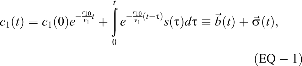
with the 2 exponential terms weighted by the initial concentration and by the source.
An aerosol source that instantaneously releases into the volume can be modeled mathematically as the generalized function, δ(t), which is zero everywhere except t = 0 and
which is of the same form as the c1(0) term in EQ-1. So rather than solving for the c1(0) term (or more generally,
For a rectangular source “[ ]” with
Note that the second equation can be obtained by setting t2 to t in the third equation. Once the source is done emitting, the exponential decay is at the same rate
Validation with Recent Data from Soft-Walled Enclosures in ABSL-4
The exponential decay rate
where v1 is the volume of the ABSL-4 room and r10 is the high-efficiency particulate air (HEPA) filter flow rate leaving the room. When the soft-walled enclosure HEPA filter was running inside the ABSL-4 room, the rate estimated experimentally was
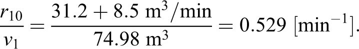
The approximation in the model is equivalent to even mixing between the enclosure and the room (ie, simply a larger single HEPA filter for the ABSL-4 room). To more appropriately model the concentration when the soft-walled enclosure is being used requires the 2-volume model, which is presented later.
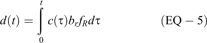
Dose Calculations and Integration with Earlier Work
From a safety perspective, the cumulative exposure to the concentration (ie, dose) is a better measure of risk than concentration directly. We define dose d(t) as a function of concentration c(t), exposure duration, breathing rate br , and retention factor fR :
Obviously, br
and fR
could be more complex (eg, time or aerosol particle-size dependencies). Unless noted otherwise, we assign bR
= 15 [L/min] = 0.25 [L/s] and fr
= 1, as assumed in Bennett et al.
2
A conservative estimate of dose with no air changes, r
10 = 0, is also usually determined. For our simple 1-volume model of concentration,
For a rectangular source from EQ-3,
Table 1 provides a comparison of terminology from Dimmick et al 3 and Bennett et al 2 with what is utilized in the MBAHA model. In some cases, the experiment-driven definitions have simplifying assumptions as compared with the MBAHA model.
Comparison of Model Definitions with Terminology Utilized in Other Publications.
Abbreviation: CFU, colony-forming units.
An assumption of prompt dispersal (eg, spray factor from Bennett et al
2
) across the entire working volume simplifies the models by eliminating time as a source parameter. This is treated as the delta source case in the MBAHA model and utilizes the more general definition by Dimmick et al
3
of source strength Sm for a single volume
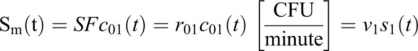
This approach allows spray factor (SF) from Bennett et al
2
to map simply to
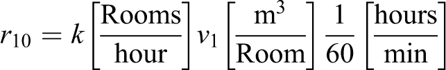
The parameters k for room changes per hour [AC/H], Sm for source strength, and SF for spray factor found in Dimmick et al 3 map to the MBAHA model as

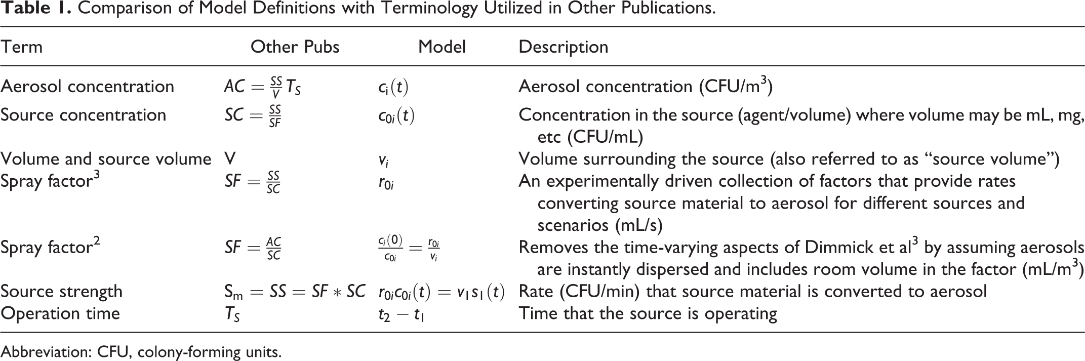
and use the values Sm = 10 000 and v 1 = 1000 m3. For a source that is continuously spraying (ie, a rectangular source with r 10 > 0, 0 = t 1 and t < t 2 from EQ-3) the concentration in a single volume room is

The concentration from EQ-8 is plotted in Figure 1 and is identical to the graph of concentration found as Figure 2 in Dimmick et al3(p260) (note the special case for k = 0, producing a concentration of
Utilizing equation 8 to reproduce the concentration results of Dimmick et al.3(p260) AC/H, air changes per hour; CFU, colony-forming units.
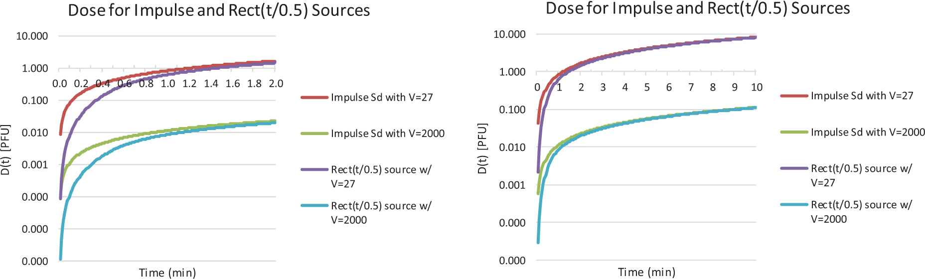
Comparison of dose models on 2- and 10-minute scales. The delta source is equivalent to the model used in Dimmick et al, 3 but the boxcar source implements the stated assumptions. On a 10-minute time scale, the results are essentially the same. PFU, plaque-forming units.
We also consider the dropped flask accident scenario assessed in Bennett et al.2(p663) The original concentration is given by the product of the source concentration (5 × 10⁹ colony-forming units [CFU] /mL) and the spray factor (5.3 × 10⁻⁷ mL/m3) or 2650 CFU/m3 = 2.65 CFU/L. The air change rate is 12 h-1, breathing rate br = 15 L/min. Using this concentration as constant over exposure times of 30 seconds and 10 minutes, Bennett et al estimate dose as 19.9 = 2.65*15*30/60 and 398 = 2.65*15*10 CFU, respectively.
In our time-varying model of dose, the delta source matches the assumption that the aerosol instantaneously disperses across the volume of the room so
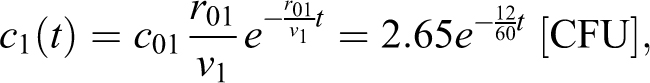
and the associated dose is
For 12 air changes per hour, we model that the dose at 30 seconds and 10 minutes is estimated as 11.6 and 171.9 [CFU]. As we show, at 10 minutes the 12 room air changes per hour have reduced the dose by more than a factor of 2.3 versus a room with no air flow (398 [CFU]). The ratio of reduced dose due to increased air flow is less for the 30-second dose (1.7 = 19.9/11.6).
Time to Reach a Specific Dose
Because we have an analytic expression for dose (EQ-6) and
or time to reach a specific concentration cc from occurrence of a delta source (with EQ-2):
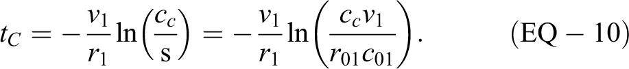
Therefore, to determine the time tf in minutes to remove a fraction f (say 0.9) of the original concentration, use
This can be used to produce a table of the fraction removed as a function of air changes per hour (note that the conversion to minutes requires a scaling of 60), shown in Table 2. In comparing this with Table 3.2 of the Health and Safety Executive Advisory Committee on Dangerous Pathogens,4(p51) we observe a typo in the 0.9999 column where the values for 0.99999 appear; the correct values are in Table 2 here.
Time in Minutes to Remove Fraction of Initial Concentration with Equation 11 Scaled by 60 for AC/H Units.
Abbreviation: AC/H, air changes per hour.
Time to remove fraction of initial concentration: t = –60*ln(1 – f) / ACH [min].
Proximal and Distal Exposure
Dimmick et al3(pp258-259) provide a sample source that generates aerosol for 0.5 minutes, 109 plaque-forming units (PFU)/mL, laboratory room volume v
1 = 2000 ft3, spray factor 5 × 10⁻⁷ mL/min, bR
= 0.3 ft3/min breathing rate, and fR
= 0.3 retention factor. This provides a source strength of 500 PFU/min = (109 PFU/mL) (5 × 10⁻⁷ mL/min). Two scenarios were considered in the paper:
A worker remains proximal to the source (within 3 ft or a volume of 27 ft3). For a room with no air flow, this results in a local concentration of 9.26 PFU/ft3 = (500 PFU/min)(0.5 min)/(27 ft3). The dose accumulated in 2 minutes is estimated as 1.67 PFU = (9 PFU/ft3)(0.3 ft3/min)(0.3)(2 min). A worker in the same laboratory volume but for 10 minutes and distal to the source (not within 3 ft) results in a diluted concentration of 0.125 PFU/ ft3 = (500 PFU/min)(0.5 min)/(2000 ft3). The dose accumulated in 10 minutes is estimated as 0.1125 PFU = (1.3 PFU/ft3)(0.3 ft3/min)(0.3)(10 min).
The calculations in Dimmick et al 3 begin once the aerosol source has completed generation and are equivalent to the MBAHA model of a delta source in a laboratory with no flow leaving the volume. Comparing the source output for the assumptions in Dimmick et al 3 with the rectangular source described that has duration of 0.5 minutes in a single volume shows the expected difference during the time that the rectangular source is generating particles (ie, concentration and dose are lower until the rectangular source catches up to the delta source). The delta source assumption therefore provides the more conservative dose estimate, as used in Dimmick et al 3 and shown in Figure 2 with 2- and 10-minute time scales.
To compare the value of being away from a source, the same delta source was utilized and the dose modeled for hemispherical volumes with radii ranging from 1 to 5 ft with a 1-ft increase in the radius of a hemisphere for each calculation (Figure 3). As expected, the closer to a source, the more reduction in dose there is for each foot moved away.
Comparison of calculated dose received for each foot away from the source. Calculated by increasing the volume of an enclosing hemisphere.
Material Balance Method for Multiple Volumes
Consider a system with n volumes vi [m3] (eg, laboratory rooms, biosafety cabinets, soft-walled enclosures), each with particle concentration c i(t) [particles/m3], 1 ≤ i ≤ n. As shown in Figure 4, the volumes are interconnected with airflow rij [m3/min] leaving v i and entering v j, ri 0 [m3/min] leaving vi through HEPA filtration (ie, a sink for the associated ri 0 ci (t) particles leaving the system), and a source producing particles entering vi with source concentration c 0i (t) [particles/m3] and source rate (also known as spray factor) r 0i [m3/min] (eg, virus shed by large animals), where t, m, min, and particles are time, meters, minutes, and CFU/PFU/other appropriate particulate measure, respectively. Depending on the application, volumes for the source concentration and source rate may be better expressed in other units (eg, mL) for liquid source material and spray devices. All flow rates in this model are assumed to move volumes of particles without changing pressures. It is also assumed that particles introduced into a volume are instantaneously dispersed across the entire volume—that is, concentration in each volume is uniform.
Concentration is modeled as n interconnected volumes with particles exchanging pairwise among volumes and each volume having a HEPA filter (ie, sink) and a source. PFU, plaque-forming units.
The number of particles v i ci (t + dt) in volume v i at time t + dt, where dt is small, can be expressed as the balance of material in the system, which must be conserved (particles staying in v i, leaving to other volumes, entering from other volumes, leaving through a filter, and entering from a source):
Rearranging terms, taking the limit as dt goes to 0, and denoting the derivate with respect to time t as
This system of n equations can be represented as

by the n × 1 column vectors
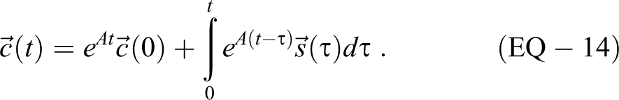
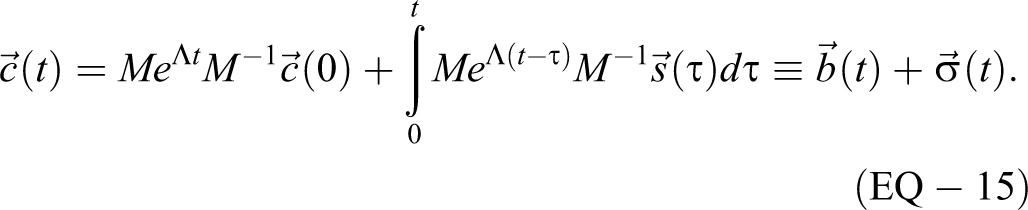
Requiring t ≥ 0, the solution of this system of differential equations is given by
There are established mathematical techniques for solving EQ-14, including eigenvalue approaches; for instance, see Dawkins
5
or Luenberger.
6
Utilizing eigenvalues λ(i) and n × 1 eigenvectors
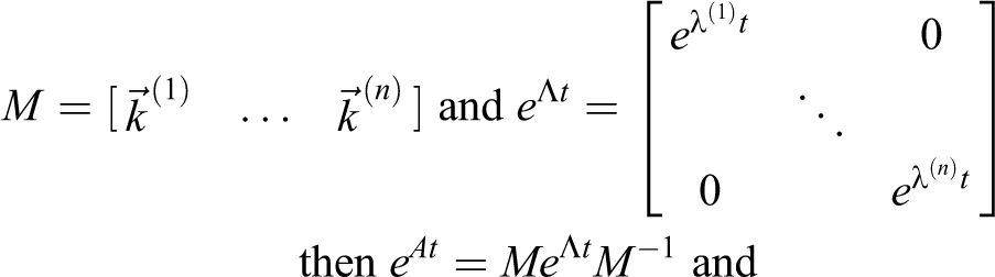
Fortunately, eigenvalue/eigenvector systems can be solved numerically (and are required for systems larger than n = 3). For 1- and 2-dimensional systems, the math to solve is straightforward, though sometimes tedious, and provides insight into the contributions of individual parameters as well as allowing additional analyses like estimation of dose. The results have already been presented for the 1-dimensional MBAHA model which is the multivolume model with n = 1,
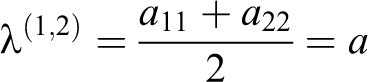
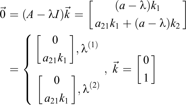
Two-Volume Material Balance Model
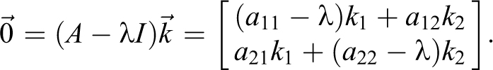
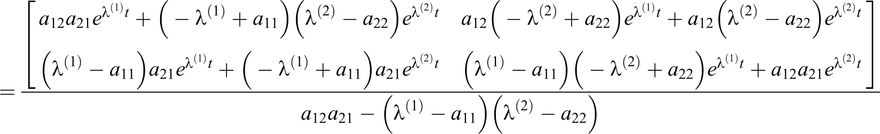
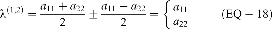
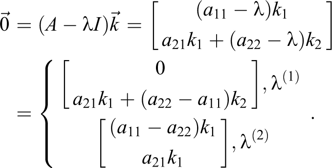
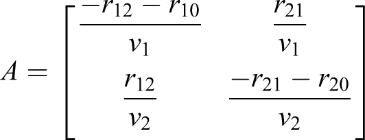
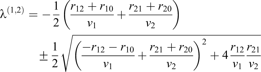
For a 2 × 2 matrix A,
To determine the eigenvectors,
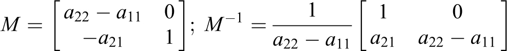
The M matrix of eigenvectors and its inverse are
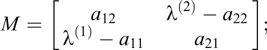
There are special cases to maintain numerical stability. The case where when no mixing occurs across volumes (a
12 = a
21 = 0) is not addressed, because this is simply 2 one-volume models. Three cases are addressed here: (1)
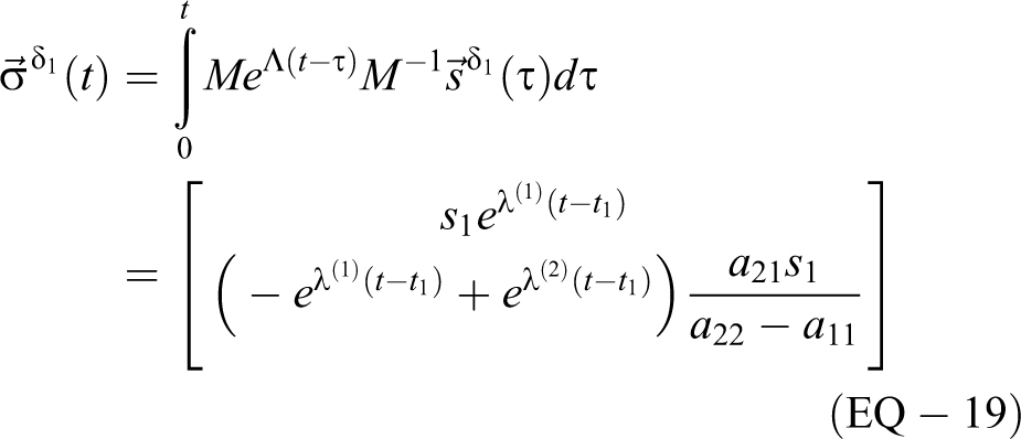
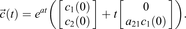
1) For
With a delta source in volume 1,
For
With a delta function at 0 =t1 = t2, s1 = c1(0), s2 = c2(0), and EQ-15:
which is the same as setting initial concentrations. Focus is then placed on
A similar approach can be utilized for a rectangular source in volume 1 that has
And with 
For a rectangular source s
2 during
With
2) For
To determine the eigenvectors
The M matrix of eigenvectors and its inverse are
For the delta function source s:
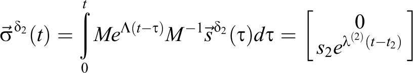
For rectangular sources, first in volume 1 alone, 
For a rectangular source s 2 located in volume 2, for t2 ≤ t (note that 0 = a12 implies 0 = r21 and volume 2 is isolated from volume 1 since the source is in volume 2):
3) For
The single eigenvector is
For this matrix A, the solution to

where
Model with No Particles Flowing from Soft-Walled Enclosure Into ABSL-4 Room
The 2 × 2 model provides an analytic framework that represents 2 volumes (eg, BSL-4 room and soft-walled enclosure), removal of particles at a specified rate for each volume (eg, HEPA filtration), arbitrary initial concentrations in each volume, instantaneous sources of particles, and continuous sources of particles with specified start and stop spray duration. Since the math is available in close form, it can be used for additional analyses, including dose estimation. The model consistency is demonstrated with the experimental measurements.
For the 2-volume, n = 2, experiment with a soft-walled enclosure in a room, use EQ-13 and EQ-16:
based on the experimental design and the observation that particles do not appear to flow from the enclosure into the room. The variables in the model are shown in Table 3.
Variables for the Model When Particles Do Not Flow from the Soft-Walled Enclosure Into the Room.
Abbreviations: ABSL, animal biosafety level; HEPA, high-efficiency particulate air.
The resulting matrix A and eigenvalues (EQ-16) are
As shown in EQ-18 and EQ-19, a source
verifying the rate in volume 1 that was approximated in EQ-10. The concentration and rate for volume 2 are a little more complicated with the difference of 2 exponentials. Since
Two-volume model with no particle flow from the soft-walled enclosure into the room, background of 1000 particles/m3, delta function sources at t = 0 of strength 3 000 000 in both volumes, and rectangular sources of strengths 200 000 000 and 400 000 000 at times 70-71 and 190-192, respectively, released in the enclosure. The model results compare favorably with the experimental data presented in Landon et al. 1 ABSL-4, animal biosafety level 4.
In a similar manner, Figure 6 presents model results of the concentration in the ABSL-4 room for (1) a 1-minute source in the ABSL-4 room with no soft-walled enclosure operating and (2) the same source inside the operating soft-walled enclosure. Also of significance in this model is the faster return to background concentration from the introduction of hallway particles for the ABSL-4 room when the enclosure HEPA filter is operating versus when the soft-walled enclosure is absent.
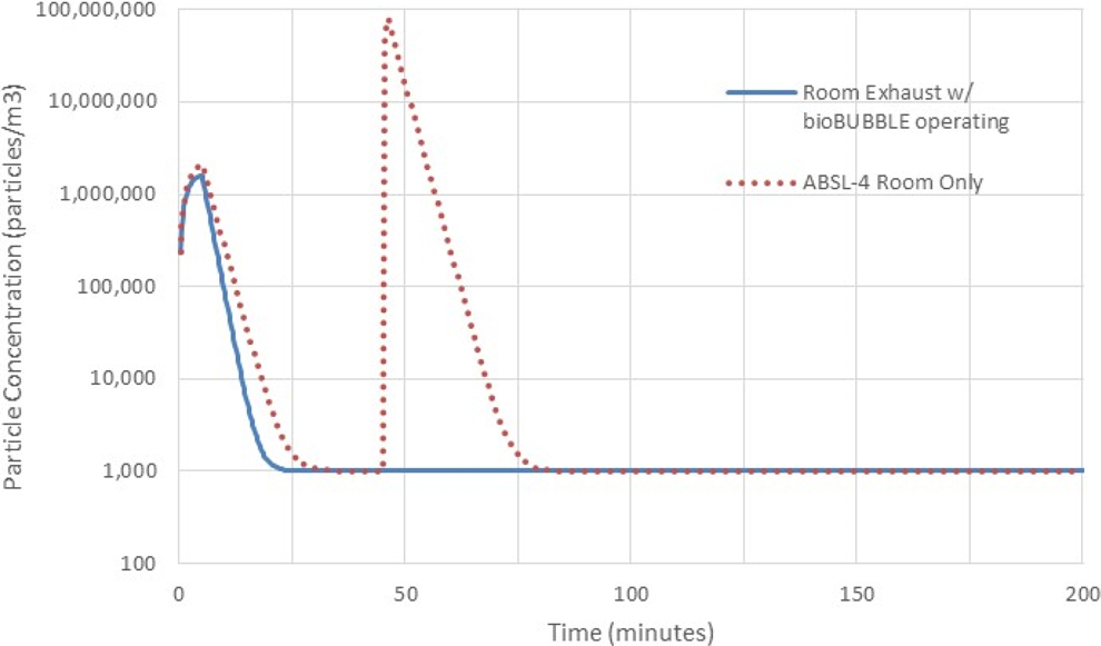
Modeled aerosol concentration in the animal biosafety level 4 (ABSL-4) room with “hallway” contamination for <30 minutes and a source from 45 to 46 minutes both with no soft-walled enclosure and with the source inside an operating enclosure. The shape and rates compare favorably with experimental data in Landon et al. 1
Model with Particles Flowing from the Soft-Walled Enclosure Into ABSL-4 Room
To investigate the potential impact of particles escaping from the soft-walled enclosure into the ABSL-4 room, 3 sources were modeled: (1) an initial concentration (delta source at time t = 0), (2) a 1-minute rectangular source inside the soft-walled enclosure, (3) a 1-minute source outside the soft-walled enclosure and a delta source outside the soft-walled enclosure. The delta source at t = 0 and 1-minute sources are scaled to match the experimental data presented by Landon et al
1
for the hallway contamination and first challenge. Two different rates of particles flowing from the soft-walled enclosure into the room (ie, r
21) are used: one set to produce a noticeable variation above background but within the maximum variation (r
21 = 0.00085, approximately 4000 particles/m3 above background) observed experimentally and with a rate equal to one-tenth of the soft-walled enclosure HEPA flow rate returned to the ABSL-4 room (r
21 = 0.85, which is also 1000 times larger than the other model calculation). The results of the model calculation are presented in Figure 7. To help explain this, EQ-12 is examined for a rectangular source in volume 2, and notice that the resulting concentration in volume 1 is weighted by
Model calculation for non-zero particle escape (r 21) from the soft-walled enclosure into the animal biosafety level 4 (ABSL-4) room for 2 different values of r 21. A 10-minute source is used in the soft-walled enclosure (60-70 minutes) to help display the different responses with the peak “leakage” concentration approximately scaling with r 21. For a 1-minute source in the ABSL-4 room, there are no significant differences in performance.
Conclusions
New experimental data on primary containment enclosures in ABSL-4 and data available from the published work of other groups were utilized to demonstrate a general material balance biocontainment model. A biocontainment room by itself (n = 1) and a biocontainment room holding a primary containment enclosure (n = 2) can both be represented by the MBAHA model to calculate concentration and integrated exposure dose. The analytic 2-dimensional model applies to all 2-volume interactions, including biosafety cabinets within laboratory rooms. The general model can be applied for an arbitrary number of volumes, n, by numerical methods on a computer that can solve matrix equations with eigenvalue decompositions.
By using simple assumptions that are amenable to spreadsheet calculation and demonstrating correlation with experimental data, a general model has been provided for biocontainment professionals to estimate particle concentration, dose, and exposure time to reach a specified dose for a wide range of scenarios.
Footnotes
Authors’ Note
The views and conclusions contained in this document are those of the authors and should not be interpreted as necessarily representing the official policies, either expressed or implied, of the US Department of Homeland Security. In no event shall the Department of Homeland Security, National Biodefense Analysis and Countermeasures Center, or Battelle National Biodefense Institute have any responsibility or liability for any use, misuse, inability to use, or reliance upon the information contained herein. The Department of Homeland Security does not endorse any products or commercial services mentioned in this publication.
Declaration of Conflicting Interests
The author(s) declared no potential conflicts of interest with respect to the research, authorship, and/or publication of this article.
Funding
The author(s) disclosed receipt of the following financial support for the research, authorship, and/or publication of this article: This work was funded under contract HSHQDC-15-C-00064 awarded by the Department of Homeland Security Science and Technology Directorate for the management and operation of the National Biodefense Analysis and Countermeasures Center, a federally funded research and development center.