Sage Journals: Discover world-class research

Abstract

A growing body of literature has examined the impact of neighborhood characteristics on Alzheimer’s disease (AD) dementia, yet the spatial variability and relative importance of the most influential factors remain underexplored. We compiled various widely recognized factors to examine spatial heterogeneity and associations with AD dementia prevalence via geographically weighted random forest (GWRF) approach. The GWRF outperformed conventional models with an out-of-bag R² of 74.8% in predicting AD dementia prevalence and the lowest error (MAE = 0.34, RMSE = 0.45). Key findings showed that mobile homes were the most influential factor in 19.9% of U.S. counties, followed by NDVI (17.4%), physical inactivity (12.9%), households with no vehicle (11.3%), and particulate matter (10.4%), while other primary factors affecting <10% of U.S. counties. Findings highlight the need for county-specific interventions tailored to local risk factors. Policies should prioritize increasing affordable housing stability, expanding green spaces, improving transportation access, promoting physical activity, and reducing air pollution exposure.

Keywords

Alzheimer's Disease dementia geographic information systems (GIS)geographically weighted random forest neighborhood characteristics spatial machine learning

Introduction

Neighborhood environments where persons living with AD dementia reside can significantly impact the progression of the disease.^1-5 For example, an age-friendly environment has been shown to be crucial for older adults with limited mobility who often spend more time in their immediate geographic surroundings.⁶ Evidence suggests that higher neighborhood deprivation is linked to lower cognitive function and increased depressive symptoms.^7,8 Mechanistically, long-term exposure to air pollution, specifically fine particulate matter (PM2.5), can trigger brain inflammation and increase the risk of cognitive decline and neuroinflammation.^9-11 Conversely, greater exposure to green spaces can reduce stress and mental fatigue, promote physical activity, and lower the risk of cognitive impairment.^12-16 Access to healthcare and community resources is crucial for managing the disease and alleviating caregiver burden.¹⁷

Geospatial analysis and modeling can provide a robust framework for examining the impact of neighboring environments on the distribution of AD dementia.^18,19 In the U.S., it has been used for the identification of spatial clusters of AD mortality rates,²⁰ spatiotemporal clusters of dementia mortality,²¹ and spatial and spatiotemporal hotspots of dementia hospitalization rates.²² However, only a limited number of geospatial modeling studies have been conducted to examine the local impact of neighborhood characteristics on AD dementia. Karway et al (2024) analyzed data from Medicare beneficiaries using geospatial methods to assess the impact of cardiometabolic diseases (CMDs), smoking, and educational attainment on the incidence of AD. They computed county-level AD incidence, adjusted for age, sex, and race using the spatial Bayesian latent Gaussian approach. They reported strong agreement between the spatial patterns of AD and CMD, a moderate association with smoking, and a weak inverse relationship with educational attainment.²³ Using the same approach, Alhasan et al (2024) investigated the link between neighborhood attributes and AD dementia incidence in South Carolina. They reported that a higher AD dementia incidence was associated with poverty, air pollution, rural settings, and limited access to nutritious food.²⁴

Additionally, a limited number of geospatial models have examined the impact of socioeconomic, environmental, and lifestyle characteristics on AD dementia distribution. One widely used model to assess the regional impact of these variables on various health outcomes is geographically weighted regression (GWR),^25,26 which relies on several challenging assumptions, such as local linearity between outcome and predictors,²⁷ and is sensitive to outliers and multicollinearities.²⁸ In contrast, random forest (RF), a nonlinear and nonparametric decision tree-based model, is not based on statistical assumptions and is less prone to overfitting and outliers.^29,30 Nevertheless, non-spatial machine learning models such as RF, Boosted Regression Trees or Neural Networks do not inherently account for spatial heterogeneity. Geographically weighted random forest (GWRF) is a recently developed spatial machine learning algorithm that can address these limitations.³¹ Conceptually, like GWR, the GWRF is calibrated using RF instead of ordinary least squares (OLS) regression and can address linearity and spatial dependence and does not rely on distributional assumptions.³² Moreover, while spatial machine learning models like Geographically Weighted Artificial Neural Networks can handle nonlinearity and spatial non-stationarity, GWRF offers more straightforward implementation and interpretation.³³

Spatial variants of RF have been previously applied to model COVID-19,²⁸ hypertension,³⁴ malaria,³⁵ asthma,³⁶ physical inactivity,³⁷ and type 2 diabetes.³² However, to our knowledge, studies have yet to examine spatial nonlinear machine learning models to study the prevalence of AD dementia. The National Institute on Aging (NIA) Health Disparities Research Framework advocates for the use of multidisciplinary methodologies to achieve health equity in aging research.³⁸ This framework organizes a spectrum of spatial factors, including environmental, sociocultural, and behavioral elements, to address health disparities, identify intervention targets, and elucidate causal pathways to health outcomes in aging populations.³⁸ Here, we compile various socioeconomic, environmental, and lifestyle variables together with related health outcomes as predictors to address the following research questions:

1. How does the spatial variability of socioeconomic, environmental, and lifestyle factors influence AD dementia prevalence at the county level in the U.S.?

2. How does the performance of GWRF compare to widely used spatial (GWR) and nonspatial (RF, OLS) models in explaining or predicting AD dementia prevalence?

3. How do the most influential variables vary across counties, and how their regional importance is ranked?

Our study extends previous geospatial research on AD dementia by being the first to apply a spatial nonlinear machine learning model to analyze its regional prevalence across the U.S. The findings can help public health policymakers to develop more relevant interventions to reduce disparities of AD dementia prevalence in the U.S. rather than a one-size-fits-all policy that might not be efficient on a broader scale.

Methods

Data Collection and Preparation

The estimated prevalence of AD dementia, serving as the outcome variable, was sourced from Dhana et al (2020) at the county level across the continental U.S.³⁹ This data comprises county-specific estimates for adults aged 65 and older, adjusted on demographic characteristics such as age, sex, race/ethnicity, and education, and was computed from cognitive data from population-based studies and the National Center for Health Statistics.

We collected various predictors (n = 24) previously shown to be associated with AD dementia based on the articles of Livingston et al (2020)⁴⁰ and Alhasan et al (2024),²⁴ and domain knowledge. These predictors were categorized into four main risk factor domains: socioeconomic, environmental, lifestyle, and other health outcomes, all at the county level (n = 3032) in the continental U.S. (Table 1).

Table 1.

Predictors Used in This Study.

Domain	Variable	Source
Socioeconomic	Below 150% poverty (%)	ACS
	Unemployed (%)	ACS
	Housing cost-burdened (%)	ACS
	No health insurance (%)	ACS
	Civilian with a disability (%)	ACS
	Mobile homes (%)	ACS
	Occupied housing with more people than rooms (%)	ACS
	Households with no vehicle (%)	ACS
	Households without a computer with internet access (%)	ACS
	Limited access to healthy foods (%)	County health rankings and roadmaps
Environmental	NDVI	MODIS
	Annual average estimates of outdoor concentrations of O₃	CACES
	Annual average estimates of outdoor concentrations of CO	CACES
	Annual average estimates of outdoor concentrations of NO₂	CACES
	Annual average estimates of outdoor concentrations of PM2.5	CACES
Lifestyle	Age-adjusted prevalence rates of binge drinking	BRFSS
	Age-adjusted prevalence rates of current smoking	BRFSS
	Age-adjusted prevalence rates of lack of leisure-time physical activity	BRFSS
Other health outcomes	Age-adjusted prevalence rates of depression	BRFSS
	Age-adjusted prevalence rates of obesity	BRFSS
	Age-adjusted prevalence rates of cognitive disability	BRFSS
	Age-adjusted prevalence rates of diagnosed diabetes	BRFSS
	Age-adjusted prevalence rates of hearing disability	BRFSS
	Age-adjusted prevalence rates of high blood pressure	BRFSS

Variables that describe vulnerable communities before, during, and after disasters were developed by the Center for Disease Control and Prevention (CDC) as the social vulnerability index (SVI).⁴¹ The SVI is constructed using county-level variables obtained from the American Community Survey (ACS) 2016-2020. The estimated rates per county were included for the following SVI variables: below 150% poverty, unemployed, housing cost-burdened, no health insurance, mobile homes, occupied housing with more people than rooms, households with no vehicle, and households without a computer with internet access. More comprehensive descriptions of variables are available from the CDC/ATSDR SVI 2020 Documentation.⁴² Additionally, limited access to healthy foods was sourced from County Health Rankings and Roadmaps.⁴³

To assess the impact of air pollution on AD dementia prevalence, annual average estimates of outdoor concentrations of air pollutants such as O₃, CO, NO₂, and PM2.5 were used. These data were estimated using a land use regression model and retrieved from the Center for Air, Climate, and Energy Solutions (CACES) through a partnership with the Environmental Protection Agency.⁴⁴ Moreover, remotely sensed normalized difference vegetation index (NDVI) was obtained from Moderate Resolution Imaging Spectroradiometer (MODIS) satellite imagery to represent vegetation density on the ground with a 500 m spatial resolution. NDVI values are calculated from Red (R) and Near Infrared (NIR) spectral bands as (NIR-R)/(NIR+R), ranging from −1 to +1, with higher values indicating denser vegetation cover.⁴⁵ Zonal statistics function in ArcGIS Pro 3.3 (ESRI, Redlands, CA) Spatial Analyst Extension was used to compute the average NDVI per county across the continental U.S.

The age-adjusted prevalence of lifestyle variables per county was extracted from the CDC PLACES dataset, derived from the Behavioral Risk Factor Surveillance System (BRFSS), using a validated method for small-area estimation.^46,47 BRFSS is the primary system for health-related telephone surveys nationwide, gathering information from U.S. residents about their health behaviors and chronic conditions.⁴⁸ The lifestyle variables encompassed the age-adjusted prevalence rates of binge drinking, current smoking, and lack of leisure-time physical activity. Additionally, the age-adjusted prevalence rates for various health outcomes, including depression, obesity, cognitive disability, diagnosed diabetes, hearing disability, and high blood pressure, were sourced from the same repository.

All collected data were compiled at the county level across the continental U.S. and were joined to the administrative boundary shapefile of counties sourced from the U.S. Census Bureau’s TIGER/Line repository.⁴⁹ Counties with several missing variables were removed from the geodatabase, resulting in a final set of n = 3032 counties. The linear correlations between the predictors were examined, and the highly correlated variables (|r| > 0.8) and those with high multicollinearity (ie, variance inflation factor (VIF) > 7.5) were excluded.⁵⁰ The final compiled geodatabase was projected to the USA Contiguous Albers Equal Area Conic projection, and the coordinates of the centroid for each county were added to the dataset using the Calculate Geometry function in ArcGIS Pro 3.3 for further geospatial modeling.

Linear Models

OLS

The baseline OLS model was employed to investigate the relationship between AD dementia prevalence and the predictors. This model has several assumptions, such as spatial stationarity across the study area, linear relationships, independence of observations, normality, random distribution of errors, and is sensitive to outliers. However, spatial dependencies can violate independence and randomness assumptions in practice.⁵¹ The mathematical descriptions of the OLS model have been provided in Supplemental File S1.

GWR

To address spatial heterogeneity, geographically weighted regression (GWR), an extension of OLS, was utilized.⁵² Mapping the locally estimated coefficients can help reveal hidden spatial patterns and the local influence of predictors on AD dementia prevalence.⁵³ Nevertheless, GWR retains assumptions of local linearity and independence of observations and remains sensitive to outliers.²⁷ Additionally, local multicollinearity can lead to instability in the parameter estimates.⁵⁴ The mathematical descriptions of GWR model have been provided in Supplemental File S1.

Nonlinear Models

Random Forest (RF)

In contrast to linear models, RF and its variants do not depend on specific relationship assumptions for the variables,²⁹ making them well-suited for capturing nonlinear relationships and interactions between variables.⁵⁵ RF is a non-parametric machine learning algorithm used for both classification and regression tasks.^29,56,57 We randomly divided the entire dataset into two portions: a training set (2/3 of the data) and an out-of-bag (OOB) set (1/3 of the data). Using the training set, numerous unpruned regression trees were constructed through bootstrap sampling (ie, random sampling with replacement) and the random selection of a subset of variables.⁵⁸ The prediction accuracy was computed for each tree, and the final output was the average prediction from all regression trees.⁵⁹

The OOB data, which was not used during the training process, were used for two primary purposes: (1) evaluating the goodness of fit and overall model accuracy using metrics such as mean square error (MSE), coefficient of determination (R²), and mean absolute error (MAE),⁶⁰ and (2) determining the relative importance of each variable.²⁸ To assess variable importance, the values of each variable in the OOB set were randomly permuted, and the OOB error was recalculated. The variable was deemed important if the OOB MSE error increases (%IncMSE) with the permuted values. The greater the increase, the more influential the variable is in predicting AD dementia prevalence.³¹ A detailed description of the RF is provided elsewhere.^29,58

Geographically Weighted Random Forest (GWRF)

Although RF addresses the limitations of linearity assumptions and susceptibility to outliers in GWR, it remains a global model and fails to capture spatial heterogeneity.⁶¹ The GWRF has recently been developed to overcome the stationary assumption of RF and the limitations of the GWR model.⁶² Similar to GWR, GWRF involves locally calibrated models rather than a single global model. GWRF addresses spatial heterogeneity by computing local RF using nearest neighbors for each location based on the spatial weight matrix.⁶³ An adaptive kernel was used to identify an optimal number of nearest neighbors due to various sizes of counties and uneven distribution of centroid of counties in the U.S.³¹ Detailed discussion on GWRF can be found elsewhere.⁶²

To enhance GWRF interpretability, permutation feature importance was used to rank the local variable importance for each county based on the %IncMSE. Further, we mapped the local variable importance to better understand where, and to what extent each variable affects AD dementia prevalence geographically.²⁸ Moreover, we estimated and mapped the local residuals and local goodness-of-fit statistics for training and OOB samples to assess the model performance in different regions. Consistent with other studies,^29,30,34 we used the OOB method to assess model accuracy instead of relying on a separate validation set. The OOB method allows for internal validation during the RF algorithm run by measuring prediction error through bootstrap aggregating. This approach facilitates the calculation of the OOB MSE and R². While both OOB and cross-validation are valid techniques for model validation, OOB is computationally more efficient as it evaluates model performance during training.^29,30

Hyperparameter Tuning

RF and GWRF are less susceptible to overfitting due to the creation of many slightly different regression trees.^29,64 They are robust prediction models when the hyperparameters are appropriately tuned, especially with large datasets.²⁹ To mitigate overfitting, we conducted a randomized grid search to optimize key RF hyperparameters using a dataset of 3032 samples. The tuned parameters included the number of features considered at each split (mtry), the fraction of data used per tree (sample.fraction), tree depth (max.depth), the minimum required samples at a leaf node (min.node.size), and the total number of trees (num.trees).^28,32 A 10-fold cross-validation method was used to determine the optimal hyper-parameters from all possible combinations. We also used these hyperparameters for GWRF. Moreover, the optimal bandwidth (maximum number of neighbors to calibrate local models) in GWRF was selected based on minimized OOB error.⁶² To further reduce overfitting, we limited the number of variables, acknowledging the constraints of county-level data, where the number of available data points is limited. After an initial RF training and tuning phase, we removed features with low importance scores (<10%).

We applied the Getis-Ord Gi* statistics to assess the clustering of high (hotspots) or low (cold spots) residual values within the entire dataset.^65,66 Mathematical descriptions of the Getis-Ord Gi* statistics have been provided in Supplemental File S1. All statistical analyses were conducted using randomForest, SpatialML, and CARET packages in R, with mapping performed in ArcGIS Pro 3.3.

Results

Preliminary descriptive statistics showed that the AD dementia prevalence (%) in the continental U.S. ranged from 5.6% in Lovington County, Texas, to 18.4% in Presidio County, Texas. The mean prevalence rate (adjusted for age, sex, race/ethnicity, and education) was 11.17%, with a standard deviation of 1.43%. The highest rates were predominantly found in southern states, including North Carolina, South Carolina, Georgia, (southern) Florida, Tennessee, Alabama, New Mexico, and (southern) Texas. The states with the lowest (mean) prevalence rates, respectively, were Utah (9.70%), Vermont (9.76%), and Idaho (9.87%), while those with the highest (mean) rates were Mississippi (13.10%), South Carolina (12.46%), and Louisiana (12.42%). Among the 24 initial predictors, four variables (ie, below 150% poverty, the age-adjusted prevalence of cognitive disability, diagnosed diabetes, and high blood pressure) were removed due to a high correlation with other variables or high VIF. After an initial RF training and tuning phase, we removed the variables with low importance scores (<10%). In Supplemental Table S1 and Figure S1, we present the correlation coefficients for the 13 final predictors, all of which are below the threshold of |0.8|, with VIFs under 7.5, indicating low multicollinearity.

Overall, nonlinear models (ie, RF and GWRF) demonstrated better fit and accuracy than linear models (ie, OLS and GWR). In terms of R² for the training dataset, the RF model had the worst performance (R² = 55.3%, MAE = 0.74, RMSE = 0.95), while the GWRF model had the best performance, with R² = 89.8% and the slightest error (MAE = 0.34, RMSE = 0.45). However, overfitting using the training dataset for nonlinear models is likely. Table 2 presents the evaluation metrics for both the training and OOB datasets.

Table 2.

Comparative Performance of the Models for AD Dementia Prevalence Rates in the US.

	Evaluation metrics (training data)			Evaluation metrics (OOB data)
Model	R²	MAE	RMSE	R²	MAE	RMSE
OLS	58.8%	0.69	0.91	NA^a	NA	NA
GWR	79.6%	0.44	0.58	NA	NA	NA
RF	55.3%	0.74	0.95	51.6%	0.76	0.99
GWRF	89.8%	0.34	0.45	74.2%	0.52	0.72

^aNot applicable.

To avoid overfitting before fitting the RF and GWRF models, we tested various combinations of hyper-parameter values through 10-fold cross-validation. The optimal hyperparameters were based on the adaptive kernel, bandwidth = 216 nearest neighbors, ntree = 1000, mtry = 6, sample.fraction = 0.3, min.node.size = 9, and max.depth = 4. For comparison, these parameters were fixed for both the training and OOB datasets of RF and GWRF models. Based on the OOB accuracy assessment, GWRF demonstrated significantly improved performance, showing a 34.5% increase in R² (Table 2). Additionally, due to the local implications and interpretations of GWRF, such as spatially varying relationships, local feature importance, flexible bandwidth selection, and integration with GIS for visualization and targeted decision-making, GWRF was used for further inferences.

According to permutation-based feature importance, the variable “Households with no Vehicle” was the most significant contributor (highest %IncMSE), followed by “Binge Drinking”, “Obesity”, “Physical Inactivity”, “Depression”, “PM2.5”, and “Mobile Homes”. However, among these 13 variables “No Health Insurance” was the least contributing variable to AD dementia prevalence. Figure 1 depicts the relative importance of variables to AD dementia prevalence.

Figure 1.

The relative importance of variables to AD dementia prevalence using permutation-based feature importance. A higher increase in MSE (%IncMSE) corresponds to higher importance.

The percentage of “Mobile homes” was the leading primary factor for the prevalence rate of AD dementia in most U.S. counties (n = 602, 19.9%). “NDVI” was the most influential factor in Central and Northern U.S. counties (n = 528, 17.4%), notably in Minnesota, Wisconsin, Missouri, and Oklahoma. “Physical inactivity” was the primary factor in south and southwestern counties (n = 391, 12.9%), predominantly in Arizona, New Mexico, Colorado, Utah, and southern Texas. “Households with no vehicle” was the main influential factor in (n = 342, 11.3%) of U.S. counties, particularly in most counties of Arkansas, Delaware, New Jersey and Illinois. Figure 2A illustrates the geospatial distribution of local primary factors of AD dementia prevalence across the U.S. along with the corresponding county counts as shown in Figure 2B.

Figure 2.

(A) Geospatial distribution of local primary factors associated with AD dementia prevalence across the U.S. (B) County-level counts for these factors.

The local effects of the top important variables were mapped, regardless of their primary status. ‘NDVI’ had the largest and most widespread impact in northern and central states, with a small cluster of counties in Texas, while having the lowest impact in the eastern and western regions. ‘Mobile Homes’ significantly influenced AD dementia prevalence in the northern and northeastern U.S., particularly in North Dakota, South Dakota, Pennsylvania, and New York, with the least impact in the south, northwest, and central regions. ‘Physical inactivity’ had the highest impact in the southern half of the U.S., notably in New Mexico, Arizona, Colorado, Louisiana, Mississippi, and South Carolina. ‘Depression’ most affected the southern half of the U.S., particularly California, Virgina and North Carolina and had the least impact on the northern states. ‘Obesity’ almost showed the same geographic pattern as ‘Physical Inactivity’. ‘PM 2.5’ had the most significant effects in the western half of the U.S., especially in northern Colorado, Wyoming, Arizona, and Nevada, and northeastern states. ‘Binge drinking’ and ‘Households with no vehicle’ exhibited nearly identical geographic patterns, with the highest impacts in southern states, particularly Alabama and Missouri, and the lowest impacts in the western and northern U.S. Figure 3 illustrates the local impact of the top variables on AD dementia prevalence in the U.S.

Figure 3.

The local impact of the top variables on AD dementia prevalence in the US.

The local R² of the GWRF model in explaining the variance of AD dementia prevalence ranged from 0.04 to 0.84 (median = 0.43, standard deviation = 0.16). The model tended to perform better in most counties in the southern, and northeastern regions (local R² > 0.7), while it underperformed in the central and northwestern U.S. (local R² < 0.2). Figure 4A illustrates the local R² of the GWRF model. The Getis-Ord Gi* analysis showed that the residuals of the GWRF model were mainly randomly distributed, with a few hotspots or cold spots indicating areas of overprediction or underprediction (Figure 4B).

Figure 4.

The geospatial distribution of (A) Local R2 of the GWRF model and (B) Getis-Ord Gi* hotspots/cold spots of residuals.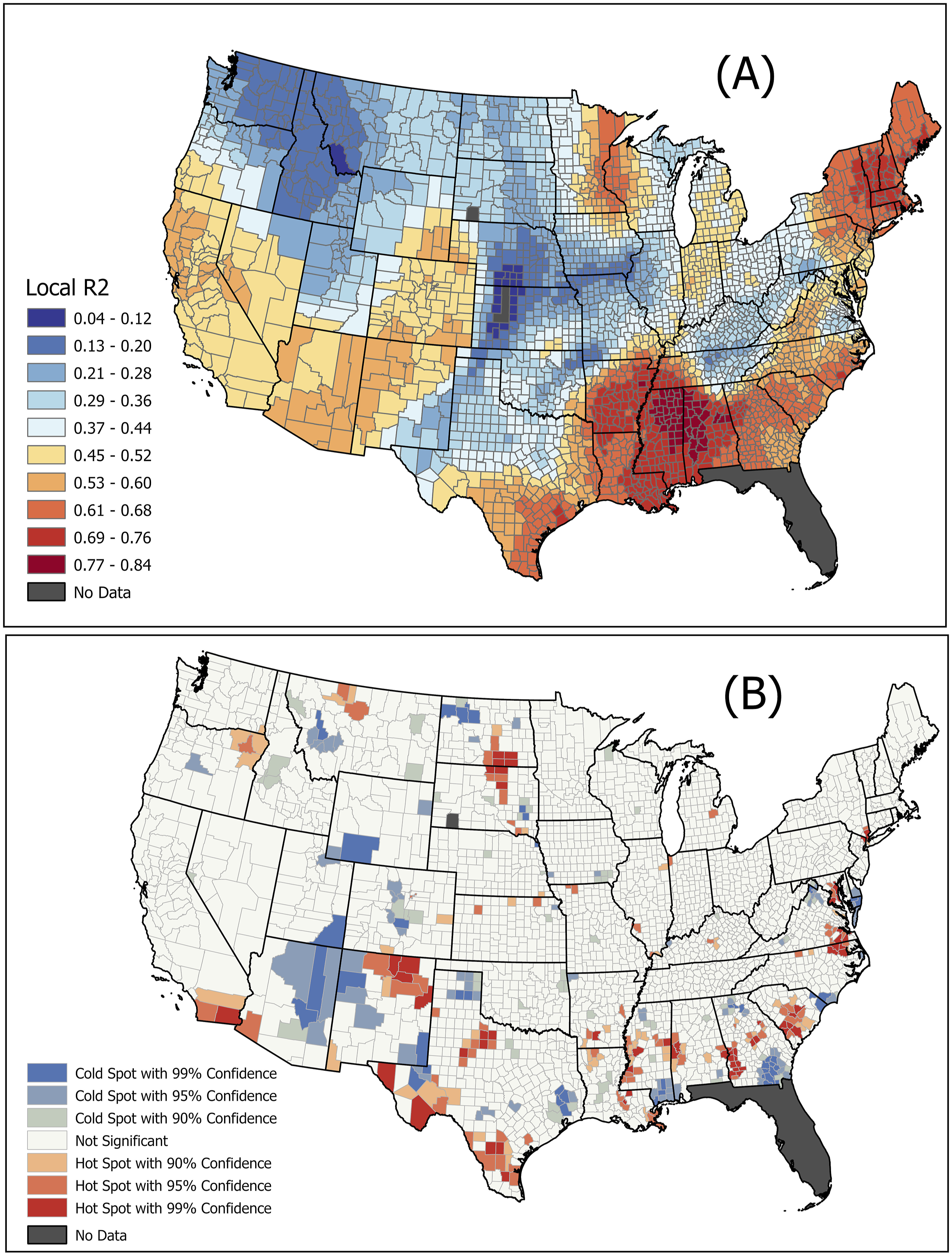

Discussion

Inspired by the NIA’s Health Disparities framework³⁸ and leveraging the foundational work by Livingston et al (2020),⁴⁰ we compiled a geodatabase of socioeconomic, environmental, and lifestyle variables along with other pertinent health outcomes at the county level in the continental U.S. Utilizing advanced spatial technologies such as GIS, remote sensing, spatial statistics, and machine learning model, we conducted a geospatial machine learning modeling of the distribution of AD dementia prevalence to better understand the local impacts of these variables in the continental U.S. The results of our study can guide interventions such as enhancing green spaces to improve cognitive health, reducing air pollution, and promoting physical activity through initiatives, for instance, for mobile home communities. The findings of this study can serve as the foundational baseline to support the development of cost-effective, place-based interventions and more refined policy development across the nation.

We sourced the AD dementia prevalence data from the study by Dhana et al (2023).³⁹ The advantage of using this data, as compared to conventional estimates relying on medical reports, claims, and national surveys, is its mitigation of significant underestimation, particularly among racial and ethnic minority groups. Conventional methods often miss cases due to discrepancies between data sources and systemic diagnostic biases. In contrast, the data used in this study incorporated findings from a diverse population-based study and adjusted for demographic variations (ie, age, sex, race/ethnicity, and education) at the county level, providing a more accurate assessment of the factors impacting AD dementia prevalence in the U.S.³⁹ African American and Hispanic older adults face a potentially 2-fold higher risk of AD dementia.⁶⁷ Therefore, the involvement of racial and ethnic minority groups in AD clinical research is emphasized.^68,69

Geospatial modeling of AD dementia remains relatively sparse, with conventional geospatial linear models like GWR constrained by local linearity, sensitivity to outliers, and multicollinearity.^27,28 Thus, our study adopted a nonlinear spatial approach to circumvent these limitations while incorporating variable interactions, resulting in superior performance to conventional linear models. Our findings confirmed previous research on other health outcomes using GWRF.^36,70 Although the model exhibited proper performance in most counties, it showed low goodness-of-fit in central and northwest U.S. counties, indicating the necessity for integrating additional critical variables and enhancing data quality.

Recent studies have shown the influence of environmental factors on AD dementia, including NDVI^71-73 and criteria air pollutants.^74-76 The permutation-based feature importance analysis suggested that among environmental factors, NDVI was found to be the most important factor in 17.4% of U.S. counties. Counties most influenced by this factor lie in the northern and central regions. Numerous studies have linked NDVI, or neighborhood greenness, to improved cognitive function and MRI results.¹² A 13-year cohort study involving over 1.1 million older adults from 2001 to 2014 indicated that an increase of one interquartile range in surrounding greenness was associated with a 4%-5% decrease in premature mortality from all neurodegenerative diseases, including AD.⁷⁷ However, one study found that this association is only significant for those with low genetic risk.⁷⁸ The protective effect of NDVI likely due to its ability to improve air quality, increase physical activity, and reduce stress,⁷⁹ while also enhancing cortical thickness, reducing ventricular size, and promoting neuroprotection, all of which may help mitigate AD risk.⁸⁰ Although NDVI is among the most influential factors in local modeling, it is not highly ranked in the global model. This discrepancy likely stems from methodological differences between global and local models. Local models, trained exclusively on neighboring data, are more sensitive to spatially clustered factors, whereas these localized effects become diluted in the global model. This sensitivity to local patterns is a key advantage of spatial modeling, allowing for the detection of trends that may be obscured in a global analysis.

PM 2.5 emerged as the other important environmental variables and the primary factors in 10.4% of U.S. counties, notably in northeastern and western states. This concurs with previous studies associating air pollution with cognitive decline.^81,82 PM 2.5, typically composed of heavy metals such as nickel, lead, cadmium, arsenic as well as organic carbon, can easily cross the blood-brain barrier and reach the central nervous system.^83,84 They can induce systemic inflammation, cell death, and DNA damage in the human brain by producing reactive oxygen species, which are critical for developing AD dementia.^85,86

Lack of leisure-time physical activity was identified as the most important modifiable lifestyle variable in explaining AD dementia prevalence. It was found as the primary variable in 12.9% of U.S. counties, particularly affecting New Mexico, Arizona, Colorado, Louisiana, and Mississippi. A review article of various study designs indicated that higher levels of physical activity are linked to a lower risk of late-life dementia. Physical activity can enlarge prefrontal and hippocampal brain areas, potentially mitigating memory impairments.⁸⁷ Possible reasons for the regional impact might include access to recreational facilities, cultural attitudes toward physical activity, and environmental factors that either promote or hinder an active lifestyle. For instance, a cross-sectional analysis of data from 50 884 women revealed that those residing in areas with the highest exposure to greenness were more inclined to participate in higher levels of physical activity (more than 67.1 MET hours per week) compared to those in areas with the lowest level of greenness.⁸⁸ ‘Binge drinking’ was another most important lifestyle variable that impacted AD dementia prevalence and the primary important variable in 9.5% of U.S. counties. A 25-year follow-up analysis among a cohort of 554 Finnish twins aged 65 years and older at the time of assessment revealed that midlife binge drinking was associated with a relative risk of 3.2 for dementia.⁸⁹ ‘Binge drinking’ can markedly worsen cognitive deficits.⁹⁰ A review study investigated how binge drinking is associated with the development of cognitive impairment among young adults in the UK. They found deficits in brain regions such as the frontal lobe, temporal lobe, and hippocampus. However, the studies lacked sufficient evidence to generalize the findings.⁹¹

Among the socioeconomic factors, ‘Mobile homes’ and ‘Households with no vehicle’ were identified as the most significant variables impacting the prevalence of AD dementia. These factors were primary variables in 19.9% and 11.3% of U.S. counties, respectively. While the exact mechanisms linking ‘Mobile homes’ to AD dementia are unclear, possible explanations include the increased socioeconomic stress faced by residents due to financial instability, limited healthcare access, and increased exposure to air pollution,⁹² —as mobile homes are typically found in low-income rural areas with limited access to interstate highways or public transit—⁹³ all of which can contribute to cognitive decline. Additionally, ‘Households with no vehicle’ can exacerbate isolation and restrict access to healthcare services and social activities, all of which are crucial for maintaining cognitive health, thereby increasing the prevalence of AD dementia.

While this study offers valuable insights, it does have its limitations. The data utilized in this study were primarily based on model-derived estimations of AD dementia prevalence and telephone survey responses from BRFSS, which are susceptible to recall and social desirability biases. The AD dementia prevalence data obtained from³⁹ focused on three major racial/ethnic groups (Black/African American, Hispanic, and White) and simply assumed that other races (ie, Asian American and American Indian/Alaska Native individuals) have a similar risk to White individuals. The AD dementia data may also be subject to selection biases, particularly due to the underrepresentation of racial/ethnic groups in clinical diagnoses, which could skew both prevalence estimates and diagnosis rates at the county level. Evidence of such bias is highlighted by Lennon et al (2022),⁹⁴ who used data from the National Alzheimer’s Coordinating Center and found that Black participants in AD research studies had 35% lower odds of receiving a dementia diagnosis at the initial visits than White participants. Additionally, due to the ecological fallacy, the conclusions cannot be extended to the sub-county or individual levels and should only be interpreted at the county level. Another limitation that might reduce the statistical power of the analysis is the absence of various key variables in certain states, notably Florida, and particularly Alaska and Hawaii, where each has a racial and ethnic minority group of approximately 40%. This led to the exclusion of these states from the analysis. While GWRF captures local spatial variations, its findings may not transfer well if key predictors, data distributions, or geographic characteristics differ. Differences in spatial scale can further affect its generalizability. Compared to linear models, GWRF only captures the relative contribution of each explanatory variable to AD dementia prevalence through variable importance, without assessing the actual effects of these variables. To enhance interpretability, future work could integrate spatial models with methods like Shapley Additive Explanations, which would provide a clearer understanding of the effects of explanatory variables.⁹⁵ Moreover, it should be acknowledged that the feature importance technique used in this study can be impacted by inter-feature correlation and multicollinearity, which can lead to misleading importance scores as permuting one feature may not accurately reflect its individual impact due to the correlated variables. Although we included a selection of well-recognized variables, future research should incorporate distinctions between rural and urban settings and consider the built environment and social isolation variables. Additionally, conducting research at finer spatial scales while maintaining a national scope is crucial for more targeted interventions. Subsequent research should involve spatial causal inference and mediation analyses to identify mediators and mechanisms.

Conclusions

In conclusion, our findings underscore the considerable spatial variability in the factors associated with AD dementia prevalence across U.S. counties. This suggests that local and regional governments should implement targeted interventions based on specific regional variables. For example, some areas may benefit from prioritizing improving green space and reducing air pollution, while others might focus on modifying lifestyle variables such as increasing physical activity and reducing binge drinking. Moreover, the fit of the local model highlights the urgent need for more comprehensive data collection and analysis to better understand how disparities impact AD dementia prevalence. Together, these insights can pave the way for more nuanced research and targeted interventions to mitigate the prevalence of AD dementia in the U.S.

Supplemental Material

Supplemental Material - Alzheimer’s Disease Dementia Prevalence in the United States: A County-Level Spatial Machine Learning Analysis

Supplemental Material for Alzheimer’s Disease Dementia Prevalence in the United States: A County-Level Spatial Machine Learning Analysis by Abolfazl Mollalo, PhD, George Grekousis, PhD, Hermes Florez, MD, PhD, Brian Neelon, PhD, Leslie A. Lenert, MD, and Alexander V. Alekseyenko, PhD in American Journal of Alzheimer’s Disease & Other Dementias®

Footnotes

Acknowledgments

The authors sincerely thank Dr. Andreana Benitez for her insightful feedback on an earlier version of this manuscript.

ORCID iD

Abolfazl Mollalo

Statements and Declarations

Funding

The authors disclosed receipt of the following financial support for the research, authorship, and/or publication of this article: AM and AVA are supported by the South Carolina SmartState Endowed Center for Environmental and Biomedical Panomics (CEABP); AVA is supported by South Carolina Cancer Disparities Research Center (SC CADRE) from NIH/NCI U54 CA210962.

Conflicting Interests

The authors declared no potential conflicts of interest with respect to the research, authorship, and/or publication of this article.

Data Availability Statement

Data sharing is not applicable as no new data were generated or analysed during this study.

Supplemental Material

Supplemental material for this article is available online.

References

Y-T

Brayne

Liu

, et al. Neighbourhood environment and dementia in older people from high-middle-and low-income countries: results from two population-based cohort studies. BMC Public Health. 2020;20:1-12.

Bagheri

Mavoa

Tabatabaei-Jafari

, et al. The impact of built and social environmental characteristics on diagnosed and estimated future risk of dementia. J Alzheimers Dis. 2021;84:621-632.

Chen

Lee

Huang

. Neighborhood built environment associated with cognition and dementia risk among older adults: a systematic literature review. Soc Sci Med. 2022;292:114560.

Cerin

Barnett

Shaw

, et al. From urban neighbourhood environments to cognitive health: a cross-sectional analysis of the role of physical activity and sedentary behaviours. BMC Public Health. 2021;21:2320.

Kramer

Cutty

Knox

Alekseyenko

Mollalo

. Rural-urban disparities of Alzheimer’s disease and related dementias: a scoping review. Alzheimers Dement. 2025;11:e70047.

Grove

. Ageing as well as you can in place: applying a geographical lens to the capability approach. Soc Sci Med. 2021;288:113525.

Vassilaki

Aakre

Castillo

, et al. Association of neighborhood socioeconomic disadvantage and cognitive impairment. Alzheimers Dement. 2023;19:761-770.

Powell

Buckingham

Larson

, et al. Association of neighborhood-level disadvantage with Alzheimer disease neuropathology. JAMA Netw Open. 2020;3:e207559.

Yung

KKL

. Air pollution and Alzheimer’s disease: a systematic review and meta-analysis. J Alzheimers Dis. 2020;77:701-714.

10.

Lin

Chen

Lin

Chen

Huang

. Air pollution is associated with cognitive deterioration of Alzheimer’s disease. Gerontology. 2022;68:53-61.

11.

Alemany

Crous-Bou

Vilor-Tejedor

, et al. Associations between air pollution and biomarkers of Alzheimer’s disease in cognitively unimpaired individuals. Environ Int. 2021;157:106864.

12.

Besser

. Outdoor green space exposure and brain health measures related to Alzheimer’s disease: a rapid review. BMJ Open. 2021;11:e043456.

13.

Jackson

. Greenspace inversely associated with the risk of Alzheimer’s disease in the mid-Atlantic United States. Earth. 2021;2:140-150.

14.

Yuchi

Sbihi

Davies

Tamburic

Brauer

. Road proximity, air pollution, noise, green space and neurologic disease incidence: a population-based cohort study. Environ Health. 2020;19:1-15.

15.

Chen

Zhang

Grekousis

, et al. Examining the importance of built and natural environment factors in predicting self-rated health in older adults: an extreme gradient boosting (XGBoost) approach. J Clean Prod. 2023;413:137432.

16.

Huang

Xiao

Grekousis

, et al. Greenness-air pollution-physical activity-hypertension association among middle-aged and older adults: evidence from urban and rural China. Environ Res. 2021;195:110836.

17.

Iriarte

Jimenez

. A caregiver must be healthy to be able to care. Am J Geriatr Psychiatry. 2021;29:473-475.

18.

Mollalo

Knox

Meng

Benitez

Lenert

Alekseyenko

. Geospatial analysis of the association between Medicaid expansion, minimum wage policies, and Alzheimer’s disease dementia prevalence in the United States. Information. 2024;15:688.

19.

Bagheri

Wangdi

Cherbuin

Anstey

. Combining geospatial analysis with dementia risk utilising general practice data: a systematic review. J Prev Alzheimers Dis. 2018;5:71-77.

20.

Amin

Yacko

Guttmann

. Geographic clusters of Alzheimer’s disease mortality rates in the USA: 2008-2012. J Prev Alzheimers Dis. 2018;5:231-235.

21.

. Detecting spatiotemporal clusters of dementia mortality in the United States, 2000–2010. Spat Spatiotemporal Epidemiol. 2018;27:11-20.

22.

Ornstein

Morrison

Liu

. Spatiotemporal patterns of hospitalizations among older adults with Co-presence of cancer and dementia in US counties: 2013–2018. J Appl Gerontol. 2024;43:601-611.

23.

Karway

Faust

Racette

, et al. Investigating epidemiologic and geospatial patterns of Alzheimer’s disease in the Medicare population across the United States (P2-9.002). Neurology. 2024;102:3671. AAN Enterprises.

24.

Alhasan

Larson

Lohman

, et al. Features of the physical and social neighborhood environment and neighborhood-level Alzheimer’s disease and related dementia in South Carolina. Environ Health Perspect. 2024;132:027013.

25.

Mollalo

Vahedi

Rivera

. GIS-based spatial modeling of COVID-19 incidence rate in the continental United States. Sci Total Environ. 2020;728:138884.

26.

Fotheringham

Crespo

Yao

. Geographical and temporal weighted regression (GTWR). Geogr Anal. 2015;47:431-452.

27.

Wheeler

Tiefelsdorf

. Multicollinearity and correlation among local regression coefficients in geographically weighted regression. J Geogr Syst. 2005;7:161-187.

28.

Grekousis

Feng

Marakakis

Wang

. Ranking the importance of demographic, socioeconomic, and underlying health factors on US COVID-19 deaths: a geographical random forest approach. Health Place. 2022;74:102744.

29.

Breiman

. Random forests. Mach Learn. 2001;45:5-32.

30.

Grekousis

. Geographical-XGBoost: a new ensemble model for spatially local regression based on gradient-boosted trees. J Geogr Syst. 2025;27(2).

31.

Georganos

Grippa

Niang Gadiaga

, et al. Geographical random forests: a spatial extension of the random forest algorithm to address spatial heterogeneity in remote sensing and population modelling. Geocarto Int. 2021;36:121-136.

32.

Quiñones

Goyal

Ahmed

. Geographically weighted machine learning model for untangling spatial heterogeneity of type 2 diabetes mellitus (T2D) prevalence in the USA. Sci Rep. 2021;11:6955.

33.

Hagenauer

Helbich

. A geographically weighted artificial neural network. Int J Geogr Inf Sci. 2022;36:215-235.

34.

Lotfata

Grekousis

Wang

. Using geographical random forest models to explore spatial patterns in the neighborhood determinants of hypertension prevalence across Chicago, Illinois, USA. Environ Plan B Urban Anal City Sci. 2023;50:2376-2393.

35.

Nduwayezu

Zhao

Kagoyire

, et al. Understanding the spatial non-stationarity in the relationships between malaria incidence and environmental risk factors using geographically weighted random forest: a case study in Rwanda. Geospat Health. 2023;18:1184.

36.

Lotfata

Moosazadeh

Helbich

Hoseini

. Socioeconomic and environmental determinants of asthma prevalence: a cross-sectional study at the US county level using geographically weighted random forests. Int J Health Geogr. 2023;22:18.

37.

Lotfata

Georganos

. Spatial machine learning for predicting physical inactivity prevalence from socioecological determinants in Chicago, Illinois, USA. J Geogr Syst. 2023;26:1-21.

38.

Hill

Pérez-Stable

Anderson

Bernard

. The national institute on aging health disparities research framework. Ethn Dis. 2015;25:245-254.

39.

Dhana

Beck

Desai

Wilson

Evans

Rajan

. Prevalence of Alzheimer’s disease dementia in the 50 US states and 3142 counties: a population estimate using the 2020 bridged‐race postcensal from the national center for health statistics. Alzheimers Dement. 2023;19:4388-4395.

40.

Livingston

Huntley

Sommerlad

, et al. Dementia prevention, intervention, and care: 2020 report of the lancet Commission. Lancet. 2020;396:413-446.

41.

Flanagan

Gregory

Hallisey

Heitgerd

Lewis

. A social vulnerability index for disaster management. J Homel Secur Emerg Manag. 2011;8:0000102202154773551792.

42.

CDC/ATSDR SVI.

Data and documentation download. https://www.atsdr.cdc.gov/placeandhealth/svi/data_documentation_download.html. Accessed August 11, 2024.

43.

County Health Rankings and Roadmaps . Health data. https://www.countyhealthrankings.org/health-data. accessed August 11, 2024.

44.

Kim

S-Y

Bechle

Hankey

Sheppard

Szpiro

Marshall

. Concentrations of criteria pollutants in the contiguous US, 1979–2015: role of prediction model parsimony in integrated empirical geographic regression. PLoS One. 2020;15:e0228535.

45.

Ren

Chen

Zhou

Tang

. Regional yield estimation for winter wheat with MODIS-NDVI data in Shandong, China. Int J Appl Earth Obs Geoinf. 2008;10:403-413.

46.

Zhang

Holt

Yun

Greenlund

Croft

. Validation of multilevel regression and poststratification methodology for small area estimation of health indicators from the behavioral risk factor surveillance system. Am J Epidemiol. 2015;182:127-137.

47.

Greenlund

Wang

, et al. Peer reviewed: PLACES: local data for better health. Prev Chronic Dis. 2022;19:E31.

48.

Pierannunzi

Balluz

. A systematic review of publications assessing reliability and validity of the Behavioral Risk Factor Surveillance System (BRFSS), 2004–2011. BMC Med Res Methodol. 2013;13:1-14.

49.

The U.S. Census Bureau. TIGER/Line shapefiles. https://www.census.gov/geographies/mapping-files/time-series/geo/tiger-line-file.html. accessed August 11, 2024.

50.

Franke

. Multicollinearity. Wiley International Encyclopedia of Marketing. John Wiley and Sons; 2010.

51.

Fotheringham

Yue

. Examining the influences of air quality in China's cities using multi‐scale geographically weighted regression. Trans GIS. 2019;23:1444-1464.

52.

Fotheringham

Brunsdon

Charlton

. Geographically weighted regression. The Sage handbook of spatial analysis. 2009;1:243-254.

53.

Rivera

Mollalo

. Spatial analysis and modelling of depression relative to social vulnerability index across the United States. Geospat Health. 2022;17:1132-1143.

54.

Fotheringham

Oshan

. Geographically weighted regression and multicollinearity: dispelling the myth. J Geogr Syst. 2016;18:303-329.

55.

Cheng

De Vos

Zhao

Yang

Witlox

. Examining non-linear built environment effects on elderly’s walking: a random forest approach. Transport Res Transport Environ. 2020;88:102552.

56.

Mollalo

Sadeghian

Israel

Rashidi

Sofizadeh

Glass

. Machine learning approaches in GIS-based ecological modeling of the sand fly Phlebotomus papatasi, a vector of zoonotic cutaneous leishmaniasis in Golestan province, Iran. Acta Trop. 2018;188:187-194.

57.

Mollalo

Vahedi

Bhattarai

Hopkins

Banik

. Predicting the hotspots of age-adjusted mortality rates of lower respiratory infection across the continental United States: integration of GIS, spatial statistics and machine learning algorithms. Int J Med Inform. 2020;142:104248.

58.

Biau

Scornet

. A random forest guided tour. Test. 2016;25:197-227.

59.

Afanador

Smolinska

Tran

Blanchet

. Unsupervised random forest: a tutorial with case studies. Journal of Chemometrics. 2016;30:232-241.

60.

Breiman

. Out-of-bag estimation. Technical Report. UC Berkeley, Department of Statistics;1996.

61.

Hengl

Nussbaum

Wright

Heuvelink

GBM

Gräler

. Random forest as a generic framework for predictive modeling of spatial and spatio-temporal variables. PeerJ. 2018;6:e5518.

62.

Georganos

Kalogirou

. A forest of forests: a spatially weighted and computationally efficient formulation of geographical random forests. ISPRS Int J GeoInf. 2022;11:471.

63.

Santos

Graw

Bonilla

. A geographically weighted random forest approach for evaluate forest change drivers in the Northern Ecuadorian Amazon. PLoS One. 2019;14:e0226224.

64.

Zhao

Chen

Zhai

, et al. Correction for population stratification in random forest analysis. Int J Epidemiol. 2012;41:1798-1806.

65.

Getis

Ord

. The analysis of spatial association by use of distance statistics. Geographical Analysis. 1992;24:189-206.

66.

Mollalo

Mao

Rashidi

Glass

. A GIS-based artificial neural network model for spatial distribution of tuberculosis across the continental United States. Int J Environ Res Public Health. 2019;16:157.

67.

Daniel

Kleiman

Galvin

. Exploring reasons for differential vulnerability and Alzheimer’s disease risk in racial and ethnic minorities. J Alzheimers Dis. 2023;91:495-506.

68.

Rubin

Ingram

Resciniti

, et al. Genetic risk factors for Alzheimer’s disease in racial/ethnic minority populations in the US: a scoping review. Front Public Health. 2021;9:784958.

69.

Shin

Doraiswamy

. Underrepresentation of African-Americans in Alzheimer’s trials: a call for affirmative action. Front Aging Neurosci. 2016;8:123.

70.

Luo

Yan

McClure

. Distribution of the environmental and socioeconomic risk factors on COVID-19 death rate across continental USA: a spatial nonlinear analysis. Environ Sci Pollut Res Int. 2021;28:6587-6599.

71.

Brown

Aitken

Lombard

, et al. Longitudinal impacts of precision greenness on Alzheimer’s disease. J Prev Alzheimers Dis. 2024;11:1-11.

72.

Zhu

Yang

, et al. Residential greenness, air pollution and incident neurodegenerative disease: a cohort study in China. Sci Total Environ. 2023;878:163173.

73.

Tondelli

Chiari

Vinceti

, et al. Greenness and neuropsychiatric symptoms in dementia. Environ Res. 2024;242:117652.

74.

Olloquequi

Díaz-Peña

Verdaguer

Ettcheto

Auladell

Camins

. From inhalation to neurodegeneration: air pollution as a modifiable risk factor for Alzheimer’s disease. Int J Mol Sci. 2024;25:6928.

75.

Singh

Ansari

Elossaily G

Vellapandian

Prajapati

. Investigating the potential impact of air pollution on Alzheimer’s disease and the utility of multidimensional imaging for early detection. ACS Omega. 2024;9:8615-8631.

76.

Guo

Yang

, et al. Ambient air pollution and Alzheimer’s disease and other dementias: a global study between 1990 and 2019. BMC Public Health. 2025;25:371.

77.

Rodriguez-Loureiro

Gadeyne

Bauwelinck

Lefebvre

Vanpoucke

Casas

. Long-term exposure to residential greenness and neurodegenerative disease mortality among older adults: a 13-year follow-up cohort study. Environ Health. 2022;21:49.

78.

Jin

Shu

Zeng

Liang

. Interaction of greenness and polygenic risk score of Alzheimer’s disease on risk of cognitive impairment. Sci Total Environ. 2021;796:148767.

79.

Nieuwenhuijsen

Khreis

Triguero-Mas

Gascon

Dadvand

. Fifty shades of green: pathway to healthy urban living. Epidemiology. 2017;28:63-71.

80.

Zagnoli

Filippini

Jimenez

Wise

Hatch

Vinceti

. Is greenness associated with dementia? A systematic review and dose–response meta-analysis. Curr Environ Health Rep. 2022;9:574-590.

81.

Shaffer

Blanco

, et al. Fine particulate matter and dementia incidence in the adult changes in thought study. Environ Health Perspect. 2021;129:087001.

82.

Shi

Zhu

Wang

, et al. Incident dementia and long-term exposure to constituents of fine particle air pollution: a national cohort study in the United States. Proc Natl Acad Sci U S A. 2023;120:e2211282119.

83.

Shou

Huang

Zhu

Liu

Wang

. A review of the possible associations between ambient PM2. 5 exposures and the development of Alzheimer’s disease. Ecotoxicol Environ Saf. 2019;174:344-352.

84.

Rafiepourgatabi

Woodward

Salmond

Dirks

. The impact of route choice on active commuters’ exposure to air pollution: a systematic review. Front Sustain Cities. 2021;2:565733.

85.

Guo

Cheung

FMH

Yung

KKL

. The association between PM2. 5 exposure and neurological disorders: a systematic review and meta-analysis. Sci Total Environ. 2019;655:1240-1248.

86.

Rafiepourgatabi

Woodward

Salmond

Dirks

. The effect of route choice in children’s exposure to ultrafine particles whilst walking to school. Int J Environ Res Public Health. 2021;18:7808.

87.

Erickson

Weinstein

Lopez

. Physical activity, brain plasticity, and Alzheimer’s disease. Arch Med Res. 2012;43:615-621.

88.

Villeneuve

Jerrett

Weichenthal

Sandler

. Association of residential greenness with obesity and physical activity in a US cohort of women. Environ Res. 2018;160:372-384.

89.

Järvenpää

Rinne

Koskenvuo

, et al. Binge drinking in midlife and dementia risk. Epidemiology. 2005;16:766-771.

90.

Ridley

Draper

Withall

. Alcohol-related dementia: an update of the evidence. Alzheimers Res Ther. 2013;5:1-8.

91.

Thayanukulvat

Harding

. Binge drinking and cognitive impairment in young people. Br J Nurs. 2015;24:401-407.

92.

Lee

Y-C

Chang

K-Y

Mirsaeidi

. Association of county-degree social vulnerability with chronic respiratory disease mortality in the United States. Ann Am Thorac Soc. 2023;20:47-57.

93.

Zhai

. Examining the spatial and temporal relationship between social vulnerability and stay-at-home behaviors in New York City during the COVID-19 pandemic. Sustain Cities Soc. 2021;67:102757.

94.

Lennon

Aita

Bene

VAD

, et al. Black and White individuals differ in dementia prevalence, risk factors, and symptomatic presentation. Alzheimers Dement. 2022;18:1461-1471.

95.

. Extracting spatial effects from machine learning model using local interpretation method: an example of SHAP and XGBoost. Comput Environ Urban Syst. 2022;96:101845.

Supplementary Material

Please find the following supplemental material available below.

For Open Access articles published under a Creative Commons License, all supplemental material carries the same license as the article it is associated with.

For non-Open Access articles published, all supplemental material carries a non-exclusive license, and permission requests for re-use of supplemental material or any part of supplemental material shall be sent directly to the copyright owner as specified in the copyright notice associated with the article.

0.00 MB

0.72 MB