Sage Journals: Discover world-class research

Abstract

A virtual source model for Monte Carlo simulations of helical TomoTherapy has been developed previously by the authors. The purpose of this work is to perform experiments in an anthropomorphic (RANDO) phantom with the same order of complexity as in clinical treatments to validate the virtual source model to be used for quality assurance secondary check on TomoTherapy patient planning dose. Helical TomoTherapy involves complex delivery pattern with irregular beam apertures and couch movement during irradiation. Monte Carlo simulation, as the most accurate dose algorithm, is desirable in radiation dosimetry. Current Monte Carlo simulations for helical TomoTherapy adopt the full Monte Carlo model, which includes detailed modeling of individual machine component, and thus, large phase space files are required at different scoring planes. As an alternative approach, we developed a virtual source model without using the large phase space files for the patient dose calculations previously. In this work, we apply the simulation system to recompute the patient doses, which were generated by the treatment planning system in an anthropomorphic phantom to mimic the real patient treatments. We performed thermoluminescence dosimeter point dose and film measurements to compare with Monte Carlo results. Thermoluminescence dosimeter measurements show that the relative difference in both Monte Carlo and treatment planning system is within 3%, with the largest difference less than 5% for both the test plans. The film measurements demonstrated 85.7% and 98.4% passing rate using the 3 mm/3% acceptance criterion for the head and neck and lung cases, respectively. Over 95% passing rate is achieved if 4 mm/4% criterion is applied. For the dose–volume histograms, very good agreement is obtained between the Monte Carlo and treatment planning system method for both cases. The experimental results demonstrate that the virtual source model Monte Carlo system can be a viable option for the accurate dose calculation of helical TomoTherapy.

Keywords

tomotherapy Monte Carlo virtual source model

Introduction

The convolution/superposition (C/S) algorithm used in the TomoTherapy treatment planning system (TPS) for the dose calculation uses a point kernel calculated in water.¹ The algorithm inherently assumes equilibrium condition throughout the volume, and therefore under the circumstances that the assumption does not hold, large deviations (5%-7%) may occur.^2

-6 Detailed Monte Carlo (MC) modeling, as the most accurate possible dose calculation method, simulates primary and scattered photons from the linac head and multileaf collimator (MLC) and contamination electrons.^7

-10 As a result of detailed modeling of individual component, large phase space files (PSFs)-containing particle information such as energy, position, direction, charge, regions of creation, or interaction of particles at different scoring planes is generated to facilitate the patient dose calculations. However, in the case that the complete mechanical drawing is not available or the PSFs are not achievable, the virtual source model (VSM) can be a good approximation.¹¹ Actually, most of the commercial TPS including TomoTherapy uses the VSM approximation for the source modeling.^12

-19 In the VSM, it is assumed that the particles originate from a single or multiple source locations. For TomoTherapy, the common multisource approximation as seen in the source modeling of conventional linacs can be reduced to a single-source approximation in view of the fact that the contribution of scattered photons for tomotherapy is much lower than conventional linacs due to its unique design. Previously, we have developed an MC simulation system based on the single-source VSM model for the purpose of developing a patient dose verification tool.¹¹ We have demonstrated in our previous work that the single-source VSM can achieve an agreement of <2% compared with the published full MC model for heterogeneous media.

In this work, we apply our MC simulation system for TomoTherapy to an anthropomorphic phantom with similar dose constraints and planning settings as in real clinical plans and perform thermoluminescence dosimeter (TLD) point dose and film measurements to compare with the TPS and MC results. The main purpose of this work is to validate the simulation system in the real clinical environment and to evaluate the VSM to be used as a viable option for quality assurance secondary check on dose distributions calculated by TomoTherapy TPS.

Materials and Methods

Tomotherapy VSM

The MC simulation system for TomoTherapy was established and commissioned as reported in our previous work.¹¹ For completeness, we describe briefly here. The MC system uses the VSM based on the machine commissioning data that were exported from the TPS in the format of eXtensible Markup Language. In building the VSM model, the scattered photons from the linac head and beam limiting devices such as jaws and MLCs were measured together with the primary photons. With the single-source approximation, the scattered photons were assumed to originate from the primary photon source. Electron contamination was excluded from calculation due to its negligible effect as demonstrated in the full MC model of tomotherapy.^9,10 To account for the difference in penumbra and fluence of different jaw size (1, 2.5, and 5 cm), the 1-dimensional transverse profile (ie, cone profile) and 2D longitudinal profile (ie, jaw profile or jaw penumbra) for each individual jaw size were kept as part of the VSM. The effect of MLC modulation has been modeled by a transfer function called the “leaf filter.” The leaf filter is a profile that represents the fluence distribution for a given open/closed leaf configuration. Due to the tongue-and-groove and penumbral blur effect, the actual fluence transmitted to a point under the direct path of a leaf of interest (LOI) is dependent on the state of its adjacent leaves, and the state of the 2 direct adjacent leaves (1 on each side) impacts the fluence profile of an LOI. Each leaf has its own leaf filter, and thus, the VSM contains 64 leaf filters as each leaf filter represents 1 MLC leaf. Taking the beam limiting devices (primary collimator, jaws, and MLC) into account, the 2D fluence map for each projection under the MLC can be modeled as

f_{js} (s, x, y) = C (x) \times J_{js} (x, y) \times L_{F} (s, x),

where C(x) is the 1D transverse profile that is independent of the Y direction, and J_js(x, y) is the 2D longitudinal profile. L_F(s, x) is the fluence profile of a leaf configuration s= (s₁, s₂, … s_i) for a given projection. The sampling of a source particle was as follows: Its initial position was sampled from the fluence map f_js(s, x, y), as shown earlier, at the MLC exit plane. The origin of the particle was sampled from the double Gaussian distribution at the target plane.²⁰ The direction of the particle was determined as the vector connecting the origin with the initial position. The transport of the particles was carried out using our in-house MC code,²¹ which has been described in our previous work.

Measurements in an Anthropomorphic Phantom

To evaluate the accuracy of the VSM and the MC system, experiments were performed in an anthropomorphic RANDO phantom (The Phantom Laboratory, Salem, New York), which presents inhomogeneities as in clinical situations. The phantom is made of materials that emulate the different tissues in a human body, such as bone, muscle, and lungs. The phantom is sliced into 2.5 cm interval, and each slice of phantom material has a grid of holes that allows the insertion of TLDs. Treatment plans in the RANDO phantom were created as clinical plans with the same planning protocol. We used the fine grid option for both TPS and MC calculations in which the computed tomography (CT) image with original resolution of 512 × 512 pixels was downsampled to 256 × 256. To convert CT number to an MC phantom, an image value-to-density table with 4 materials (air, lung, soft tissue, and bone) was used. The material was assigned to each voxel by the predefined material density range. The uncertainty of material and density assignment was expected to introduce small dosimetric difference (<1.5%),²² which was not considered in this study.

Dose Measurements With TLD

Twenty lithium fluoride (LiF:MgTi) TLD-100 chips (Model 168; Radiation Products Design, Albertville, Minnesota) and a Harshaw TLD reader (Model 3500; Thermo Scientific, Waltham, Massachusetts) were used for this study. The dimension of the TLD is 3.2 × 3.2 × 0.9 mm³. According to the manufacturer specification, repeatability can be within 2% or better and it was verified at initial use in our institution. The full anneal of the TLDs was performed with 400° for 1 hour, followed by 2 hours at 100° before irradiation. The element correction coefficient (ECC) for each TLD was determined by exposing the TLDs to a calibration dose of 200 cGy performed against an Exradin A1SL ion chamber (Standard Imaging, Middleton, Wisconsin) using an Elekta accelerator. The ECC was used to take into account the efficiency of each TLD, and the variation in efficiency can be reduced to 1% to 2%. The TLDs were wrapped with preservative film to avoid any contamination from the phantom in irradiation. The TLDs were removed from the phantom after irradiation and set at room temperature for 3 days in order to allow time for low-energy traps to decay. They were then read with a Harshaw TLD reader.

Previous studies and observations made by other authors have shown that deviations between MC and C/S dose algorithm are more likely to occur at the regions close to air cavities or low-density tissues, bones, or high-density materials.^2,6,23 Therefore, we intentionally allocated some TLDs inside or on the border of these regions in an attempt to detect the difference when comparing the measurement to the 2 dose algorithms. Figure 1A and B shows an overview of the 20 TLD locations for the head and neck (H&N) and lung case, respectively. The planning target volume (PTV) contours were included in the figures to indicate the regions of large dose gradient.

Figure 1.

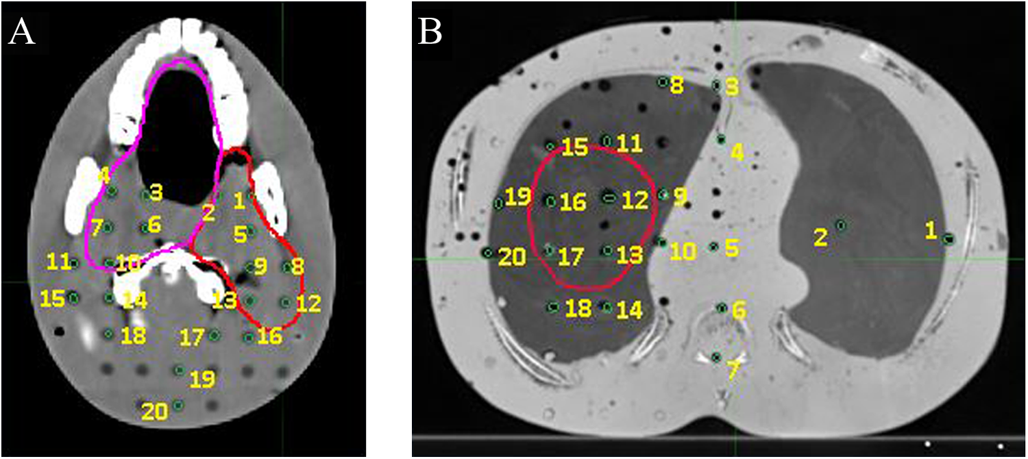
A, Illustration of TLD locations for the H&N case. B, Illustration of TLD locations for the lung case. H&N indicates head and neck; TLD, thermoluminescence dosimeter.

Radiochromic Film Measurements

Relative dose distributions were measured in the same axial plane as TLDs in the RANDO phantom with EBT3 radiochromic films (Advanced Materials, Wayne, New Jersey). The films at the axial plane were carefully aligned in parallel to the beam rotation plane. The films were scanned with a VIDAR ProDosimetry film digitizer (VIDAR Systems Corporation, Herndon, Virginia). To create a calibration curve, we delivered known doses from 0.4 to 5 Gy to the cut film pieces using TomoTherapy machine. Then, the irradiated film piece was scanned to obtain the scanner response.²⁴ We used Radiological Imaging Technology (Colorado Springs, Colorado) film analysis software to calculate the γ index^25,26 between measurement and calculation with its other built-in functions such as autoregistration.

Head and Neck Case Plan

We created a treatment plan in the RANDO phantom by mimicking a clinical case of tongue squamous cell carcinoma plan. There were 2 PTVs that include the oral cavity. The prescription was 63 Gy to the 98% of PTV1 and 56 Gy to the 95% of PTV2 volume in 30 fractions. The critical structures were the brainstem, the spinal cord, the parotids, the optic nerves, and chiasm. The planning constraints used in the planning were (1) the maximum dose to the brainstem should be less than 54 Gy, (2) the maximum dose to the spinal cord should be less than 45 Gy, (3) at least 50% of both parotids should receive dose of less than 30 Gy, and (4) the maximum dose to the optic nerves and chiasm should be less than 10 Gy. We used 2.5 cm jaw size and 0.3 pitch for planning. The modulation factor (MF) was set to 2.0, and the actual MF was 1.76. The generated plan had 28.1 active rotations (1433 projections), and the treatment duration was 337.2 seconds for each fraction.

Lung Case Plan

For the lung case, we simulated a treatment plan in the RANDO phantom with a stereotactic body radiotherapy dose regimen. A large-size PTV was drawn inside the right lung, and the prescription was 50 Gy to 98% PTV in 5 fractions. The critical structures were the spinal cord, heart, and left lung. Dose constraints were used as in the clinical setting. The field width was 2.5 cm, and the pitch was set to 0.2. The actual MF was 1.74. The generated plan had 13.2 active rotations (673 projections), and the treatment time was 286.4 s for each fraction.

In order to compare with TLD measurement, point dose has to be found out from the calculated dose distribution with the TPS and MC. As it is impossible to identify the exact position because the TLD has finite size, we contoured each TLD on the slice as a circle with the radius of 3 mm. The minimum, maximum, and mean values were calculated for the dose value inside the circle. Large difference among those values indicated large dose gradient at the contoured TLD location.

Results

Results for H&N Case Plan

We repeated the TLD dose measurements 3 times using the same TLD batch to decrease the measurement uncertainty. The average of 3 measurements was taken as the point dose value as shown in Figure 2A. The dose rate of each delivery was recorded and used for output fluctuation correction for the measurements. The minimum and maximum values at the TLD location were drawn as error bar in the figure, and the mean value was used to compare with measurement. As we can see, TLD 11, 14, and 16 were located close to the PTVs, and thus, they were at the fast dose fall-off region. The maximum difference between the minimum and maximum value within the TLD circle was as large as 7.1 Gy. Nevertheless, the mean values were within 3% of the TLD measurement. The MC and TPS results at all these 20 locations agree with the TLD measurement within 5% relative difference as shown in Figure 2B. 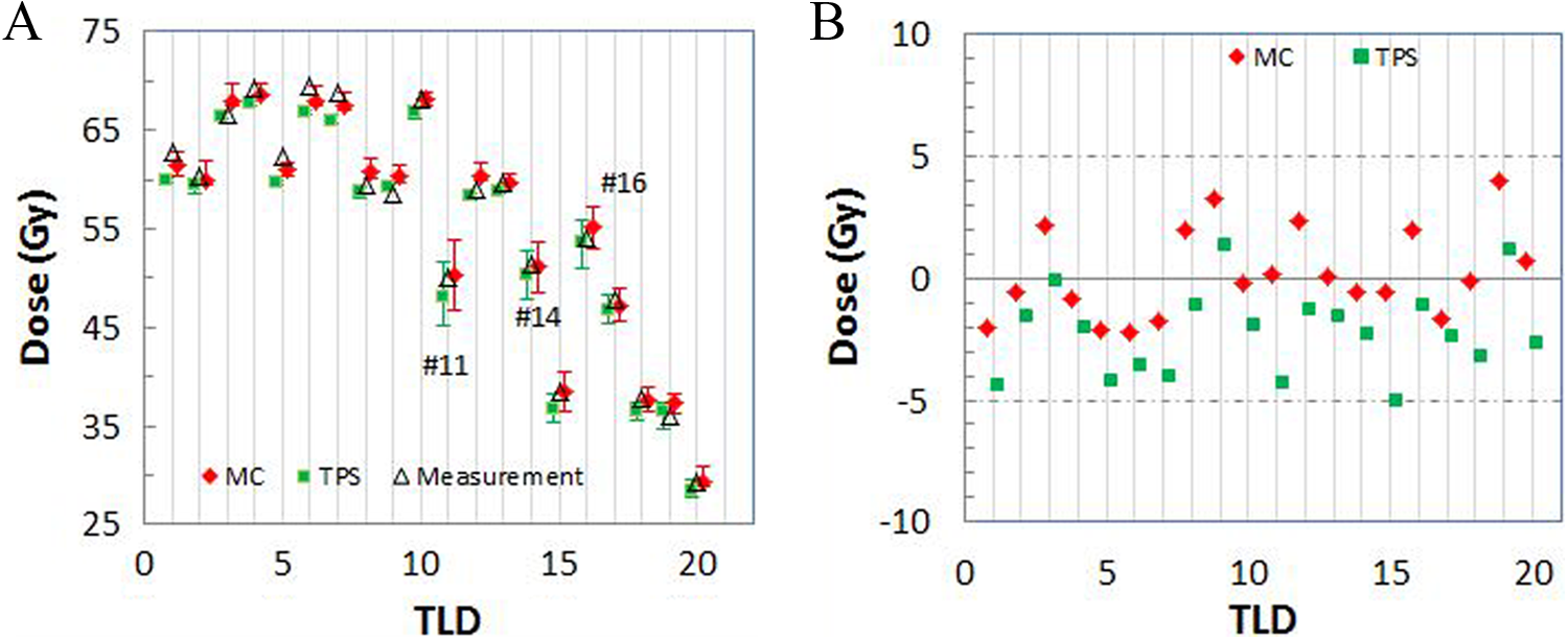The root mean square (RMS) difference, calculated as $\sqrt{\sum_{i} {(R D)}^{2} / 20}$ , where RD is the relative difference, was 1.8% and 2.8% for MC and TPS results, respectively.

Figure 2.

A, Comparison of measured and calculated TLD doses of the 20 locations for the H&N case. The MC and TPS doses were calculated as the mean dose within the TLD, which was depicted as a circle with the radius of 3 mm. The error bars stand for the minimum and maximum dose values within the TLD location. B, Percentage difference between the MC or TPS result and TLD measurement. H&N indicates head and neck; MC, Monte Carlo; TLD, thermoluminescence dosimeter; TPS, treatment planning system.

The isolines of 40, 50, and 60 Gy calculated by VSM MC and TPS are compared with the film measurement, as shown in Figure 3A and B, respectively. The film was placed at the distal end of oral cavity in the phantom slab, the same CT axial plane as shown in Figure 1A. The corresponding γ maps with 3%/3 mm criterion are shown in Figure 4A and B. The dose threshold was set to 20 cGy in order to trim out the outside region of head because the film was cut to fit in the phantom. We can see that both MC and TPS results agree with measurement in most regions. Differences are seen in the oral cavity, mandible, and dental region. Table 1 shows the passing rates using different γ index criteria. The passing rate is defined as the ratio of the number of pixels having γ index less than 1 to the total number of pixels. As we can see, the passing rates calculated by the MC method are very similar to those calculated by TPS. The high-dose gradients make the distance to agreement (DTA) very sensitive to the film registration, as we can see that the passing rate increased from 85% to 91% by increasing the DTA from 3 to 4 mm. Good agreement between the MC and TPS method was obtained for both PTVs and other critical structures except left parotid as shown in Figure 5.

Figure 3.

A, The MC-calculated planar dose compared with the film measurement. B, The TPS-calculated planar dose compared with the film measurement. The isodose lines are 40 Gy (green), 50 Gy (cyan), and 60 Gy (red), and the heavy dashed lines are film measurements in both figures. MC indicates Monte Carlo; TPS, treatment planning system.

Figure 4.

A, The γ index map between MC-calculated planar dose and the film measurement. B, The γ index map between the TPS-calculated planar dose and the film measurement. The γ index was calculated with 3%/3 mm criterion. MC indicates Monte Carlo; TPS, treatment planning system.

Table 1.

The Passing Rates Using Different γ Index Criteria Between the Calculated TPS and MC 2-Dimensional Planar Dose Distribution and the Film Measurement.

Criterion	MC				TPS
Criterion	Passing Rate, %	Mean	Max	Std Dev	Passing Rate, %	Mean	Max	Std. Dev.
3%/3 mm	85.7	0.57	2.14	0.39	85.2	0.58	2.35	0.38
3%/4 mm	91.1	0.50	1.97	0.33	91.7	0.51	1.98	0.33
4%/4 mm	95.5	0.42	1.59	0.28	95.6	0.44	1.59	0.29
5%/5 mm	98.8	0.24	1.27	0.23	99.0	0.23	1.28	0.23

Abbreviations: Max, maximum; MC, Monte Carlo; Std Dev, standard deviation; TPS, treatment planning system

Figure 5.

The cumulative DVH comparisons for PTVs and ROI structures calculated by TPS and MC method for the H&N case plan. Dashed lines represents MC and solid lines TPS. DVH indicates dose–volume histogram; H&N, head and neck; MC, Monte Carlo; PTVs, planning target volumes; ROI, region of interest; TPS, treatment planning system.

Results for Lung Case Plan

The point doses for the 20 TLD locations from the MC and TPS calculations compared with TLD measurements are shown in Figure 6A. The large error bars measuring the uniformity within the TLD location are shown for TLD 14, 15, and 18, as they are close to the PTV. However, for the mean values, both MC and TPS results are within 4% of the TLD measurement for all these 20 locations as shown in Figure 6B. The RMS of MC and TPS results is 1.1% and 1.6%, respectively.

Figure 6.

A, Comparison of measured and calculated TLD doses of the 20 locations for the lung case. The MC and TPS doses were calculated as the mean dose within the TLD, which was depicted as a circle with the radius of 3 mm. The error bars stand for the minimum and maximum dose values within the TLD location. B, Percentage difference between the MC or TPS result and TLD measurement. MC indicates Monte Carlo; TLD, thermoluminescence dosimeter; TPS, treatment planning system.

The results of isodose lines and γ index maps are shown in Figure 7A and B and Figure 8A and B. Very good agreement (passing rate > 97.8%) is obtained between the results with MC and TPS calculations and film measurement, even to the low-dose region (12 Gy, 24% of prescription). The MC presents an area in PTV having statistical noise as we show the isodose line for the prescription dose (50 Gy). The corresponding γ map shows slightly larger γ values in this area. The statistical uncertainty achieved in the simulation was 0.5%. If the statistical uncertainty is decreased further, we expect the noise can be reduced, and thus, the γ index values for that region will be improved. Comparing with measurement, the TPS, on the other hand, shows disagreement at the interface region of the chest wall and lung. The passing rates using 3 mm/3%, 4 mm/4%, and 5 mm/5% for the MC and TPS are 98.4% versus 97.8%, 99.8% versus 99.3%, and 100% versus 100%. For the dose–volume histograms, excellent agreement is obtained between the MC and TPS method for all structures except a slight difference in the left lung as shown in Figure 9.

Figure 7.

A, The MC-calculated planar dose compared with the film measurement. B, The TPS-calculated planar dose compared with the film measurement. The isodose lines are 12 Gy (gray), 20 Gy (green), 30 Gy (blue), 40 Gy (dark green), and 50 Gy (red), and the dashed lines are film measurements in both figures. MC indicates Monte Carlo; TPS, treatment planning system.

Figure 8.

Figure 9.

The cumulative DVH comparisons for PTV and ROI structures calculated by TPS and MC method for the lung case plan. Dashed lines represent MC and solid lines TPS. DVH indicates dose–volume histogram; MC, Monte Carlo; PTV, planning target volume; TPS, treatment planning system.

Discussion

An independent second check on the TPS-calculated dose or monitor units is common practice and recommended by international guidelines in radiation oncology.^27

-34 Tools such as in-house developed or commercial packages have been used for different modalities for the years past. For TomoTherapy, 3 approaches have been seen in such endeavors. One approach uses common dosimetric functions such as tissue phantom ratio and output factor (S_cp) for the central axis combined with lateral and longitudinal profiles (off-axis ratio) to calculate point doses.^27,29 The advantage of the simple analytical correction-based method is that the calculation can be very fast (within 1 minute). The other approach²⁸ uses the same dose algorithm (collapsed cone convolution) as in the TPS to calculate the patient 3D dose distribution, as in the “final dose” step in the TPS. The third approach^9,10 uses rigorous MC simulations, which takes the detailed machine information into account. This method provides the most accurate patient dose in 3 dimensions as the expense of speed as expected.

Since neither the mechanical drawing of the machine components nor the PSF was available to us, we developed a VSM in MC simulation for the dose calculation. The system automatically reads the exported DICOM CT images, radiotherapy (RT) plans, RT structures, and RT dose from the TPS and computes dose on the same CT image. Message Passing Interface (MPI) was implemented in the program so that it can run on multiple processors. Graphical user interface (GUI) was also developed for ease of use. Computing technologies such as secure shell and secure file transfer protocol were integrated so that the GUI is able to remotely execute the MC simulation in the cluster.

Good agreement (3 mm/3% criterion) was found for planar dose distributions for the lung case compared with measurement with 98% passing rate. For the H&N case, the comparison between the MC result and measurement was a little worse with the passing rate of 85.7% using the rigid criterion of 3 mm/3%, whereas the TPS gave a similar pass rate of 85.2%. By increasing the DTA to 4 mm, the passing rate was improved to 91% for both MC simulation and TPS. This indicates the alignment of calculated dose planar distribution to the film is essential as a slight shift in the high-dose gradient regions due to the apparent heterogeneity round the oral cavity could increase the γ value. The other cause may come from the slight misalignment of the film plane to the CT plane. With 4 mm/4% criterion, the passing rate for both MC simulation and TPS reached 95.5%. Large discrepancy of the dose to PTVs encompassing lung tissue between MC simulation and TPS was not observed in our lung case. This could be due to the relatively large lung PTVs in our case as the discrepancy between the collapsed cone convolution and MC dose algorithm only becomes pronounced for the small fields. The agreement was very good with deviation within 0.5% for D95 for the PTV and slightly larger difference in the contralateral lung. However, from the γ map at the measured dose plane, we did observe the larger difference between TPS and measurement at the interface region of the chest wall and lung, whereas the difference is much smaller for the MC result, although the MC simulation showed noises at the center of the PTV.

In our VSM MC method, the fluence map through the MLC is created with leaf filters, and thus, the calculation time spent on the particle generation is negligibly small comparing the calculation time due to the simulation inside the patient volume. We used 10 processors in a cluster to carry out the calculation; 10¹¹ particles were simulated for both cases, and the statistical uncertainty was achieved at 0.16% and 0.17% after 1142 minutes and 1184 minutes running time for the H&N and lung test case, respectively. If the statistical uncertainty is increased to the clinically acceptable level of 2%, we expect the simulation time reduced by 100 times, which is around 12 minutes. This time frame is clinically acceptable for performing a secondary check on TPS dose. To further facilitate the usage of our MC system on a daily basis, the implementation of the MC code with graphics processing unit acceleration is currently under development.

Footnotes

Authors’ Note

The work made use of the High Performance Computing Resource in the Core Facility for Advanced Research Computing at Case Western Reserve University.

Declaration of Conflicting Interests

The author(s) declared no potential conflicts of interest with respect to the research, authorship, and/or publication of this article.

Funding

The author(s) received no financial support for the research, authorship, and/or publication of this article.

Abbreviations

References

Mackie

Bielajew

Rogers

Battista

. Generation of photon energy deposition kernels using the EGS Monte Carlo code. Phys Med Biol. 1988;33(1):1–20. doi:10.1088/0031-9155/33/1/001.

Carrasco

Jornet

Duch

. Comparison of dose calculation algorithms in phantoms with lung equivalent heterogeneities under conditions of lateral electronic disequilibrium. Med Phys. 2004;31:2899–2911. doi:10.1118/1.1788932.

Martens

Reynaert

De Wagter

. Underdosage of the upper-airway mucosa for small fields as used in intensity-modulated radiation therapy: a comparison between radiochromic film measurements, Monte Carlo simulations, and collapsed cone convolution calculations. Med Phys. 2002;29(7):1528–1535. doi:10.1118/1.1487421.

Paelinck

Smedt

Reynaert

. Comparison of dose-volume histograms of IMRT treatment plans for ethmoid sinus cancer computed by advanced treatment planning systems including Monte Carlo. Radiother Oncol. 2006;81(3):250–256. doi:S0167-8140(06)00567-6.

Sterpin

Salvat

Olivera

Vynckier

. Monte Carlo evaluation of the convolution/superposition algorithm of Hi-Art tomotherapy in heterogeneous phantoms and clinical cases. Med Phys. 2009;36(5):1566–1575. doi:10.1118/1.3112364.

Sterpin

Tomsej

De Smedt

Reynaert

Vynckier

. Monte Carlo evaluation of the AAA treatment planning algorithm in a heterogeneous multilayer phantom and IMRT clinical treatments for an Elekta SL25 linear accelerator. Med Phys. 2007;34(5):1665–1677. doi:10.1118/1.2727314.

Belec

Ploquin

La Russa

Clark

. Position-probability-sampled Monte Carlo calculation of VMAT, 3DCRT, step-shoot IMRT, and helical tomotherapy dose distributions using BEAMnrc/DOSXYZnrc. Med Phys. 2011;38(2):948–960. doi:10.1118/1.3538922.

Jeraj

Mackie

Balog

. Radiation characteristics of helical tomotherapy. Med Phys. 2004;31(2):396–404. doi:10.1118/1.1639148.

Sterpin

Salvat

Cravens

Ruchala

Olivera

Vynckier

. Monte Carlo simulation of helical tomotherapy with PENELOPE. Phys Med Biol. 2008;53(8):2161–2180. doi:S0031-9155(08)66373-3.

10.

Zhao

Mackenzie

Kirkby

Fallone

. Monte Carlo calculation of helical tomotherapy dose delivery. Med Phys. 2008;35(8):3491–3500. doi:10.1118/1.2948409.

11.

Yuan

Rong

Chen

. A virtual source model for Monte Carlo simulation of helical tomotherapy. J Appl Clin Med Phys. 2015;16(1):4992. doi:10.1118/1.4814808.

12.

Chetty

DeMarco

Solberg

. A virtual source model for Monte Carlo modeling of arbitrary intensity distributions. Med Phys. 2000;27(1):166–172. doi:10.1118/1.598881.

13.

Luo

. Application of Monte Carlo simulation to cavity theory based on the virtual electron source concept. Phys Med Biol. 2002;47(17):3263–3274. doi:10.1088/0031-9155/47/17/314.

14.

Ondraczek

Christ

. Experimental determination of the virtual source point of high-energy electron beams for clinical application. Z Med Phys. 2005;15(4):229–234.

15.

Ravindran

. A study on virtual source position for electron beams from a Mevatron MD linear accelerator. Phys Med Biol. 1999;44(5):1309–1315. doi:10.1088/0031-9155/44/5/316.

16.

Rucci

Carletti

Cravero

Strbac

. Use of IAEA’s phase-space files for the implementation of a clinical accelerator virtual source model. Phys Med. 2014;30(2):242–248. doi:S1120-1797(13)00238-X.

17.

Sikora

Alber

. A virtual source model of electron contamination of a therapeutic photon beam. Phys Med Biol. 2009;54(24):7329–7344. doi:S0031-9155(09)16009-8.

18.

Sikora

Dohm

Alber

. A virtual photon source model of an Elekta linear accelerator with integrated mini MLC for Monte Carlo based IMRT dose calculation. Phys Med Biol. 2007;52(15):4449–4463. doi:S0031-9155(07)44566-3.

19.

Sterpin

Chen

Mackie

Olivera

Vynckier

. On the relationships between electron spot size, focal spot size, and virtual source position in Monte Carlo simulations. Med Phys. 2011;38(3):1579–1586. doi:10.1118/1.3556560.

20.

Chen

Chao

Sterpin

. A slit method to determine the focal spot size and shape of TomoTherapy system. Med Phys. 2011;38(6):2841–2849. doi:10.1118/1.3589133.

21.

Yuan

Chen

Brindle

. Investigation of nonuniform dose voxel geometry in Monte Carlo calculations. Technol Cancer Res Treat. 2015;14(4):419–427. doi:1533034614547459.

22.

Zurl

Tiefling

Winkler

Kindl

Kapp

. Hounsfield units variations: impact on CT-density based conversion tables and their effects on dose distribution. Strhlenther Onkol. 2014;190(1):88–93. doi:10.1007/s00066-013-0464-5.

23.

Madani

Vanderstraeten

Bral

. Comparison of 6 MV and 18 MV photons for IMRT treatment of lung cancer. Radiother Oncol. 2007;82(1):63–69. doi:S0167-8140(06)00631-1.

24.

Valeria

Massimo

Giuliana

. Dosimetric characterization and use of GAFCHROMIC EBT3 film for IMRT dose verification. J Appl Clini Med Phys. 2013;14(2):158–171. doi:10.1120/jacmp.v14i2.4111.

25.

Low

Harms

Mutic

Purdy

. A technique for the quantitative evaluation of dose distributions. Med Phys. 1998;25(5):656–661. doi:10.1118/1.598248.

26.

Yuan

Chen

. A gamma dose distribution evaluation technique using the k-d tree for nearest neighbor searching. Med Phys. 1998;37(9):4868–4873. doi:10.1118/1.3480964.

27.

Gibbons

Smith

Cheek

Rosen

. Independent calculation of dose from a helical TomoTherapy unit. J Appl Clin Med Phys. 2009;10(1):2772. doi:10.1120/jacmp.v10i1.2772.

28.

Nelson

Mason

Robinson

Kisling

Kirsner

. Commissioning results of an automated treatment planning verification system. J Appl Clin Med Phys. 2014l;15(5):4838. doi:10.1120/jacmp.v15i5.4838.

29.

Papanikolaou

Vazquez

. MU-Tomo: independent dose validation software for helical TomoTherapy. J Cancer Sci Ther. 2010;2:145–152. doi:10.4172/1948-5956.1000040.

30.

Ayyangar

Nizin

Saw

Gearheart

Shen

Enke

. Independent dose calculations for the corvus MLC IMRT. Med Dosim. 2001;26(2):135–141. doi:S0958-3947(01)00067-X.

31.

Caneva

Rosenwald

Zefkili

. A method to check the accuracy of dose computation using quality index: application to scatter contribution in high energy photon beams. Med Phys. 2000;27(5):1018–1024. doi:10.1118/1.598967.

32.

Duggan

Kron

Howlett

Skov

O’Brien

. An independent check of treatment plan, prescription and dose calculation as a QA procedure. Radiother Oncol. 1997;42(3):297–301. doi:S0167814097019063.

33.

Samuelsson

Hyodynmaa

Johansson

. Dose accuracy check of the 3D electron beam algorithm in a treatment planning system. Phys Med Biol. 1998;43(6):1529–1544. doi:10.1088/0031-9155/43/6/012.

34.

Julian

Malicki

. The importance of accurate treatment planning, delivery, and dose verification. Rep Pract Oncolo Radiother. 2012;17(2):63–65. doi:10.1016/j.rpor.2012.02.001.

Experimental Validation of Monte Carlo Simulations Based on a Virtual Source Model for TomoTherapy in a RANDO Phantom

Abstract

Keywords

Introduction

Materials and Methods

Tomotherapy VSM

Measurements in an Anthropomorphic Phantom

Dose Measurements With TLD

Radiochromic Film Measurements

Head and Neck Case Plan

Lung Case Plan

Results

Results for H&N Case Plan

Results for Lung Case Plan

Discussion

Footnotes

Authors’ Note

Declaration of Conflicting Interests

Funding

Abbreviations

References