
Abstract
Introduction
Lung cancer has the highest mortality rate among all cancer types globally, largely due to delayed or ineffective diagnosis and treatment. Radiomics is commonly used to diagnose lung cancer, especially in later stages or during routine screenings. However, frequent radiological imaging poses health risks, and while advanced diagnostic alternatives exist, they are often costly and accessible only to a limited, privileged population. Leveraging clinical data using machine learning (ML) and artificial intelligence (AI) enables a safer, more inclusive, and affordable solution. Due to a lack of interpretability, AI-based models for cancer diagnosis are less adopted by clinicians.
Methods
This study introduces a safe, inclusive, and cost-effective lung cancer diagnostic method using an explainable AI (XAI) model built on routine clinical data. It employs a stacking ensemble of Artificial Neural Network (ANN) and Deep Neural Network (DNN) to match the diagnostic performance of clean-data DNN models. By incorporating rare medical cases through Adaptive Synthetic Sampling (ADASYN), the model reduces the risk of missing challenging, rare-case diagnoses.
Results
The proposed XAI model demonstrates strong performance with an accuracy of 0.8558, AUC of 0.8600, precision of 0.8092, recall of 0.9282, and F1-score of 0.8646, notably improving rare case detection by over 50%. SHapley additive exPlanations(SHAP)-based interpretability highlights Erythrocyte sedimentation rate(ESR), intoxication-related factors, hemoglobin levels, and neutrophil counts as key features. The model also reveals associations, such as a link between heavy tobacco use and elevated ESR. Counterfactual explanations help identify features contributing to misdiagnoses by exposing sources of confusion in the model's decisions.
Conclusion
Given the limited dataset size and geographic constraints, this research should be viewed as a prototype and in its current form, the model is best suited as a pre-screening tool to support early detection. With training on larger and more diverse datasets, the model has strong potential to evolve into a robust and scalable diagnostic solution.
Keywords
Introduction
Carcinogenic agents are found to induce uncontrolled cellular proliferation in the pulmonary organs, resulting in the formation of malignant tumours in the lungs, leading to the culmination of lung cancer. The probability of a successful treatment outcome is positively correlated with the stage of disease detection, with earlier being better.1,2 Upon confirmation, the patient must undergo a systematic treatment to enhance the likelihood of survival. According to the Global Cancer Observatory (GLOBOCAN) 2022, the number of new cancer cases diagnosed that year was 20 million. 3 The number of deaths due to cancer in 2022 was about 9.7 million, with lung cancer being the leading cause. GLOBOCAN predicts that the number of cancer cases in 2050 will reach 35 million. While considering cancer-related mortality, lung cancer tops the chart (18.7%), followed by colorectal cancer (9.3%), liver cancer (7.8%), stomach cancer (6.8%), and female breast cancer (6.9%). Men were affected predominantly by lung, prostate, and colorectal cancers, whereas women were affected predominantly by breast, colorectal, and lung cancers.
As per the 2022 report by the American Cancer Society (ACS), there were about 117,910 and 118,830 newly diagnosed cases of lung cancer in men and women, respectively, in the United States (US). Studies by the ACS 1 reveal that the incidence of mortality resulting from lung cancer was approximately 68,820 among males and 61,360 among females. In cases where the cancer is in a localised stage, the five-year survival rate was 55%. The age group of 65 years and older exhibited the highest mortality rates for lung cancer. The incidence of lung cancer diagnosis among individuals under the age of 45 was observed to be significantly lower. According to Surveillance, epidemiology, and end results (SEER) statistics, 4 the mean age at which lung cancer was diagnosed was 70 years. The reported rate of early detection of lung cancer stands at approximately 16%. In accordance with, 3 the five-year survival rate in the event of metastasis is reported to be merely 4%. The prognosis of lung cancer is significantly influenced by both the extent of progression and the duration of time between its onset and diagnosis. Thus, successful treatment is more likely to happen when detection occurs at an earlier stage.
Radiation screening is a widely utilised non-invasive diagnostic technique for lung cancer. However, it is typically found to be applied during the advanced stages of the disease only due to initial symptoms being commonly misattributed to other health conditions.5–7 In addition, radiomics has limitations such as non-standardisation of acquisition parameters, inconsistency in radiomic methods, and limited reproducibility. Scholars are currently researching how to surmount these constraints.8,9 The repeated subjection to computed tomography (CT) imaging and low-dose computed tomography (LDCT) screening technique may increase the probability of the occurrence of solid cancers and leukemia due to cumulative exposure to ionising radiation. This is a matter of serious concern for non-cancerous patients.10–12 LDCT screening is found to have a high false positive rate (FPR), as observed in some studies.12,13 So, researchers are exploring for better alternative methods for the early detection of lung cancer.14,15
AI has the power to recognise patterns in clinical healthcare data and obtain insights from them in order to develop predictions, diagnoses, prognoses, and so on more accurately. Currently, AI-based models are being actively researched in diagnostic procedures, medication development, customised medicine, patient monitoring, and treatment protocol formation. 16 Studies have also reported that different ML and AI techniques serve as models for global practices to aid cancer research to improve clinical workflow and diagnostic accuracy, reduce human resource costs, increase the efficiency of data, and enhance treatment.17–19 Although AI has been quickly integrated into cancer research, AI-based solutions are still in their early stages. We see that only a few applications based on AI have been authorised for usage in the real world. 20 To increase these numbers, the AI models developed must be explainable and interpretable to foster trust, ensure safety and effectiveness, and adhere to regulatory and ethical standards.
One commonly used method for AI model interpretability is feature importance analysis, which gives a global perspective by assessing how the model's performance varies when the values of the features are shuffled. Layer-wise relevance propagation techniques, such as Deep Taylor decomposition, attribute the output to input features by backward propagation through the layers of the network.21,22 The drawbacks of these techniques include complexity in the deployment and the increasing difficulty of interpretation with non-linearity. Guidotti et al 23 proposed local rule-based explanations (LORE), a local interpretable predictor on a synthetic neighbourhood generated by a genetic algorithm. It derives from the logic of the local interpretable predictor a meaningful explanation consisting of a decision rule, which explains the reasons for the decision, and a set of counterfactual rules, suggesting the changes in the instance's features that lead to a different outcome. It focuses on local explanations rather than global descriptions of how the overall system works. 23 Local interpretable model-agnostic explanations (LIME) is an interpretation that typically generates an explanation for a single prediction by any ML model by learning a simpler interpretable model (for example, a linear classifier) around the prediction by generating simulated data around the instance by random perturbation and obtaining feature importance through applying some form of feature selection. The random perturbation and feature selection methods have the possibility of instability in the generated explanations for the same prediction. 24 SHAP is based on the concept of Shapley values from cooperative game theory, which provides a fair allocation of contributions among the features for a prediction. It provides additive explanations where the prediction is explained as a sum of contributions from each feature, ensuring consistency and accuracy.25,26 SHAP algorithms can be model-specific (TreeSHAP for tree-based models, DeepSHAP for neural networks). Integrated Gradients 27 is another method that assigns an importance score to each feature by integrating the gradients along the path from a baseline input to the actual input. It provides a comprehensive way to understand how each feature contributes to the model's prediction.
We should understand that an explainable AI model used to be either a complex model with “detailed understanding” requirements or a simple model with a “global perspective of the decisions made”, and thus, there exists a trade-off between the simplicity of the explanation model and the level of detail in interpretations. However, it is true that the majority of the available AI models for cancer diagnosis are not fully explainable as they are complex and work like a “black box.” This makes it difficult to explain how these models have arrived at their conclusions, and this is a problem for doctors who need to trust the AI's diagnosis and be able to explain it to patients. Thus, despite the increase in accuracy, the AI models’ lack of transparency and accountability is limiting their adoption into practice, particularly in critical applications such as cancer diagnosis.
The literature reveals numerous studies focused on developing alternatives to radiomic diagnostic models. 28 Despite these novel approaches, their implementation has been limited by high costs and the requirement for advanced technologies to extract and analyse the data. This highlights the need for more cost-effective and accessible solutions for lung cancer diagnosis.
According to an oncologist affiliated with the Cancer Institute at University College London, individuals tend to disregard persistent coughing and subsequently present at the clinic with metastatic disease. Unfortunately, at this point, the possibility of receiving effective treatment for cancer might have already diminished. 2 The preliminary indications of lung cancer are frequently perceived as typical maladies and deemed insignificant. The process of clinical staging is therefore a crucial factor in the determination of both treatment options and the likelihood of survival. The clinical guidelines should be subjected to regular revisions based on the available data to accurately identify predictors and facilitate prompt diagnosis. 8 When it comes to identifying the early signs of lung cancer, not all clinical doctors have the same level of expertise as subject matter experts.
According to research by Huang et al, 28 lymphocytes have been suggested as a potential prognostic indicator for lung cancer. Based on the findings by Wu et al, 29 the haemoglobin to red blood cell (RBC) distribution ratio may serve as a prognostic indicator for small cell lung cancer. In a recent study, Guidotti et al 23 have developed an ML model that utilises non-imaging electronic health record (EHR) data. Based on a dataset comprising 6505 patients diagnosed with lung cancer and 189,597 control subjects, the model exhibited superior accuracy compared to the Prostate, lung, colorectal, and ovarian cancer screening trial (PLCO) criteria in forecasting the occurrence of lung cancer within a one-year timeframe. These alternatives to radiation screening for the early diagnosis of lung cancer are expensive and limited in availability.
The literature demonstrates the significant potential clinical data holds for facilitating lung cancer diagnoses. 30 However, the suggested approaches are mostly restricted from common practice because they are unavailable at major healthcare centres or very expensive. So, there is a need for more research to find viable alternatives to radiation screening for the early diagnosis of lung cancer.
A review of the literature reveals that despite the huge potential clinical data hold for early diagnosis of lung cancer, the existing approaches predominantly utilise clinical data to analyse comorbid conditions 31 associated with lung cancer and predict survival rates.32,33 However, there is a noticeable gap in the development of diagnostic models specifically designed for lung cancer detection.2,5 To the best of our knowledge, no comprehensive diagnostic model leveraging clinical data has been developed or made available for deployment in medical centres to facilitate lung cancer diagnosis.
Research Challenges and Objectives
From the literature, the existing challenges are identified, which can be summarised as:
− Repetitive exposure to conventional radiomic diagnostic methods poses potential health risks of developing cancer. − Lung cancer, being an internal cancer, the initial disease symptoms are often regarded as inconsequential or assumed to be other maladies, leading to a late diagnosis of lung cancer. − Though there are novel alternatives developed for radiomic detection methods. They are not inclusive as the respective medical tests are available and affordable only to a privileged segment of the population. − Despite the huge potential clinical data hold for early diagnosis of lung cancer, the existing approaches predominantly utilise clinical data to analyse comorbid conditions associated with lung cancer and predict survival rates. − Though AI-based cancer diagnosis models are rapidly growing, they are hardly adopted into practice as medical practitioners deem them an incomprehensible black box. − While developing the AI diagnostic model, there is an increasing tendency to discard rare medical cases, which will lead to biased learning by the model, leading to the failure of detecting rare medical cases.
To address some of the above challenges, we propose to use XAI models, utilising clinical data to diagnose lung cancer. The main contributions of this research work include:
− A safe alternative to traditional radiomics-based lung cancer detection methods for the early diagnosis of lung cancer. This is inclusive and non-invasive because of the use of normal clinical data. − A key advantage of the proposed approach is its seamless integration into existing clinical workflows without the need for additional capital investment in specialised equipment or diagnostic tests. The tool leverages routinely collected clinical data, making it a cost-effective solution. Moreover, because it does not rely on sophisticated technologies or equipment typically limited to privileged healthcare settings, the model is more accessible to a broader population. − An explainable AI diagnostic model, to address the reliability and transparency concerns of healthcare practitioners. − The diagnostic model can diagnose rare medical cases as well.
Thus, in this research, we develop an explainable AI model that can interpret the model's diagnosis of lung cancer from clinical data. This can enhance early diagnosis and increase the reliability of the model's operation to facilitate timely medical intervention for lung cancer in clinical practice. The rest of the paper is organised as follows: Section 2 presents the research gap in the existing works utilising clinical data. Section 3 describes the materials and methods used for the research, including the data and models. Section 4 evaluates the performance of the models and presents the results. Section 5 explains the models’ decision-making process. Section 6 discusses the implications of this research for timely diagnosing malignancy in clinical practice. Section 6 concludes the paper.
Materials and Methods
We present this article in accordance with the transparent reporting of multivariable prediction models developed (TRIPOD) reporting checklist. 34 Figure 1 shows the architecture of the proposed diagnosis model. Each of the processes and components is explained in detail in the subsequent sections.
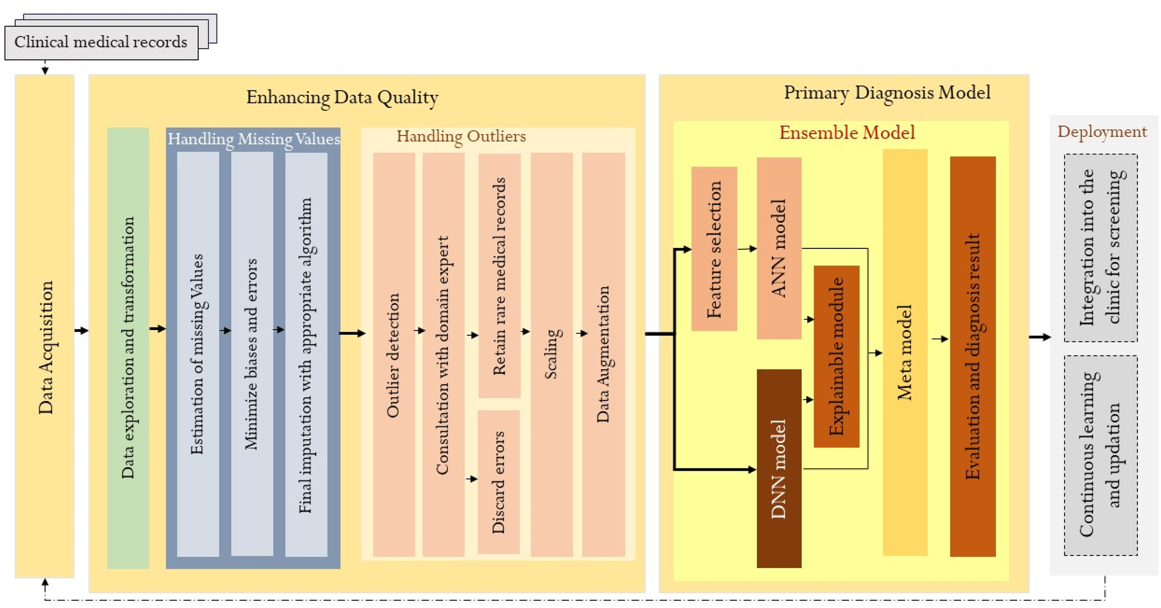
Architecture of the Proposed Diagnosis Model.
Data Collection
This research is conducted by a collaborative team of technical and medical experts in the field in line with the ethical and data collection standards outlined in. 35 This retrospective study utilised data from the Pulmonology Department of the third-largest hospital in India. It encompasses all recorded clinical observations of patients diagnosed with lung cancer as well as those with non-cancerous lung diseases between the period 2017-2019. Given the retrospective nature of the study, no prospective inclusion or exclusion criteria were applied. Instead, all available patient records meeting the diagnostic coding criteria for lung cancer or benign pulmonary conditions were included. While this approach maximises real-world representativeness, we acknowledge that the study does not adhere to pre-specified standards for data collection, such as standardised inclusion/exclusion criteria or prospective data acquisition protocols. As such, potential variability in clinical documentation and missing data are considered when interpreting the findings.
From a cohort of 743, including 378 confirmed cases of lung malignancy and 365 cases diagnosed with benign pulmonary conditions. The dataset comprised 74 independent variables and one dependent variable, with features encompassing patient demographics, clinical symptoms, and a full blood count profile. Due to the retrospective nature of data acquisition, completeness varied; only 15 records were fully complete, while 728 contained varying degrees of missing data. A total of 23 records were excluded from the analysis due to having more than 80% missing values. Appropriate data imputation and pre-processing techniques were employed to address the remaining missingness and prepare the data for analysis. 36
Patient Characteristics
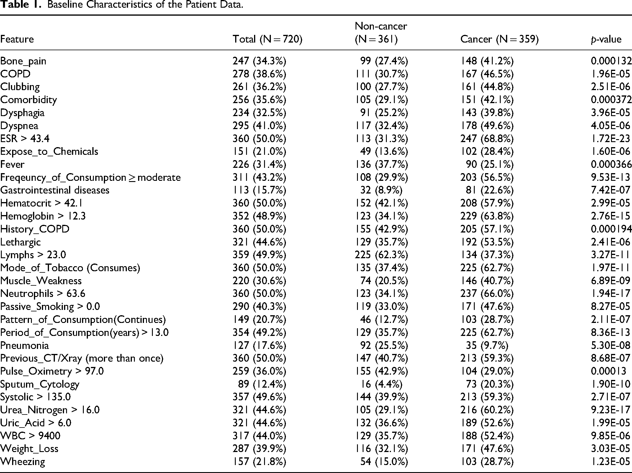
Our dataset contains patient details such as gender, age, habitual and intoxication characteristics, critical environmental checks, family history of cancer, clinical signs and symptoms, recording of history of lung diseases, clinical analysis results of blood and urine, and current disease observation. The 74 independent variables (features) include Gender, Age, Type_of_Meal, Diet_Type, Mode_of_Tobacco, Period_of_Consumption, Freqeuncy_of_Consumption, Pattern_of_Consumption, Passive_Smoking, Alcoholic, Modality_of_Cooking, Cancer_in_Family, Clean_water, Expose_to_Chemicals, Vision_Problem, Comorbidity, Previous_CT/Xray, History_TB, History_Pneumonia, History_COPD, History_Respiratory_Tract_Infection, History_Interstetial_Lungdisease, BMI Gastrointestinal, Muscle_Weakness, Slow_Tissue_Healing, Weight_Loss, Eating_Disorder, Wheezing, Chest_pain, Bone_pain, Shaking_chills, Night_sweats, Coughing_Status, Fever, Lethargic, Hoarseness_in_Sound, Limbs_swelling, Dehydration, Dyspnea, Dysphagia, Hemoptysis, Rheumatoid, Hepatomegaly, Pleural_Effusions, Clubbing, Systolic, Diastolic, Pulse, Pulse_Oximetry, Pulmonary_Hypertension, Sputum_Cytology, Spirometry, WBC, RBC, Hemoglobin, Hematocrit, Platelets, Neutrophils, Lymphs, Monocytes, ESR, Glucose_Fasting, Bacteria_in_Blood, Creatinine, Urea_Nitrogen, Uric_Acid, Urine_Protein, Blood_group, COPD, Pneumonia, TB, Myocardial_Infarct_syndrome, Coronary_Artery_Bypass. The target variable is a binary variable Cancer_class. Table 1 shows the relevant baseline characteristics of the patient data.
Baseline Characteristics of the Patient Data.
Data pre-Processing
The collected data contained mixed variables that are numeric and categorical in nature. The feature encoding technique is applied to transform categorical data. The features that have constant values for all instances are discarded. These transformations resulted in 78 input features. During the process of data exploration, it was observed that a significant number of attributes in the dataset exhibited a non-Gaussian distribution. Therefore, we used the semi-parametric multiple imputation chained equation (MICE) imputation to handle the missing values in the data. 36 MICE utilises multiple regression to examine all conditional distributions and associated regression models. 37 Then each missing attribute is predicted based on a regression equation. So, for multiple missing attribute data, there will be multiple chains of values. The missing values are initially imputed with placeholders, and then the missing records are regressed multiple times, in a cyclic manner. Subsequently, the missing value is substituted with the predicted value. This approach is recommended by Van Buuren 38 for imputing data when the sample size is greater than 400. The predicted missing values need not lie within the range of observed values.
Handling Outliers
In ML, the training data needs to be free from outliers. There is a high chance of outliers with medical data, and so they are to be handled appropriately. Outliers in medical data can arise from two causes, one by error and the other by rare medical cases. This needs to be properly differentiated with the help of a domain expert or by standard procedures. Using the density-based isolation forest method, 39 we identified the presence of 73 outliers in our data. With the guidance of the domain expert, we understood that these are not error cases but rare medical cases. Discarding rare cases in medical data for learning is not a recommended practice. Hence, we need to appropriately prepare it for the AI model by applying scaling and data augmentation. Robust scaling techniques scale the data based on the median and the interquartile range. This approach is more resilient to the presence of outliers, as it is less influenced by extreme values. Robust scaling is particularly beneficial when working with non-Gaussian data. 40 Data augmentation selectively augments the underrepresented records, helping to create more balanced and representative datasets. Synthetic minority oversampling technique (SMOTE) and adaptive synthetic sampling (ADASYN) are the two prominent methods used for data augmentation. 41 SMOTE finds the n-nearest neighbours in the minority class for each of the samples in the class. Then, it extrapolates the neighbour points and generates random data points. ADASYN is an improved version of SMOTE. ADASYN adds a random variance to the random points generated to scatter the points rather than confining them to linear extrapolation. 41 Hence, we apply the ADASYN method to augment the data.
Model Selection
Given the limitations in the volume of data available for this research, we selected the following widely used cancer diagnosis models: Logistic regression, 42 K-Nearest Neighbours (KNN), 43 Random forest, 44 Support vector machine (SVM), 45 ANN 46 and DNN. 47 We trained these classifier models with our dataset, and the performance of these diagnosis models is compared in Table 2.
Preliminary Results of the State-of-the-art Cancer Diagnosis Models on our Clinical Data.

From the preliminary results shown in Table 2, we found that the top-performing diagnosis models are DNN and ANN models. So, we focus more on these two models.
Building the AI Models
ANNs are very promising in cancer diagnosis as they have the potential to find complex patterns in data. 48 This is important in cancer diagnosis as subtle variations in blood tests, imaging scans, or a patient's medical history may hold clues about the presence or absence of cancer. Studies have shown that ANN models are achieving high accuracy rates in diagnosing various cancers, such as lung cancer, skin cancer, and so on. After exploratory analysis, we understood that our data has a complex structure. Various factors such as non-linearity, high dimensionality, interdependencies, and non-Gaussian data distributions can contribute to this structure. 49 Therefore, the structure of the data may not be easily captured by simple linear models. Therefore, we choose the ANN model, which is capable of analysing data with complex structures.
An ANN classifier consists of an input layer, one or more intermediate hidden layers, and an output layer. Each layer is composed of a number of interlinked neurons. The input layer receives the input features, and the output layer produces the final classifications. Every individual neuron employs an activation function to the summation of its inputs that have been weighted. 50 The choice of initial weights can affect how quickly the neural network converges during training. Well-selected initial weights can lead to faster convergence, reducing the time it takes for the model to learn the underlying patterns in the data. Common techniques for weight initialisation include random initialisation, Glorot initialisation, He initialisation, and so on. If all the neurons in a particular layer start with the same initial weights, they may end up learning the same features during training. This symmetry issue can hinder the model's ability to learn diverse representations and can limit its capacity. 51 Randomly initialising the weights helps the optimisation algorithm escape local minima during training. The activation function introduces non-linearity and allows the network to learn complex patterns. The rectifier linear unit (ReLU) activation function outputs the maximum non-negative value. 52
The input data is passed through the network in the forward direction, from the input layer to the output layer. The outputs of the neurons in each layer serve as inputs to the neurons in the subsequent layers. This process is called feedforward propagation, and it transforms the input data through the network to generate predictions. Each connection between neurons is associated with a weight, which represents the strength of the connection. Additionally, each neuron has a bias term, which allows the network to adjust the output independently of the input. These weights and biases are initially random and are updated during the training process. The network is trained by adjusting the weights and biases to minimise a loss function that measures the discrepancy between the predicted labels and the true labels. The backpropagation algorithm is commonly used for the training of ANNs. 50 It calculates the gradients of the loss function with respect to the model parameters and updates the weights and biases accordingly. At the output layer, to enable binary classification, the sigmoid activation function is chosen to ensure that the predicted values are between 0 and 1. Our model uses the Adam learning rate optimisation algorithm that combines the benefits of both momentum and root mean square propagation (RMSprop) for improving the model's performance. It adjusts learning rates for each parameter individually, making it well-suited for neural network optimisation. 53 Model complexity and simplicity of interpretation are two key factors to be considered while designing a diagnosis model. Therefore, we design two AI models: a simple ANN model, which learns from the feature-selected attributes based on relevance, and a DNN model, which learns from the entire data.
ANN Model
We develop a shallow ANN model that has only one hidden layer between the input and output layers. Such neural networks are simpler to train and use less computational resources. So, we need to perform a feature selection to reduce the number of features fed to the model. Leveraging the Extra trees feature selection and ranking scores, we filtered 15 relevant features as input to model. 54 The selection of 15 attributes from 78 was finalised through a subset selection approach. This is to keep our model simple and explainable.
The extra trees feature selection method assesses the significance of each feature in an ensemble model built on Extra Trees based on Gini impurity scores. Here, the higher the value, the more significant the feature. 55 The benefits of this method include the ability to handle mixed data, improved generalisation, capture of intricate feature-feature interactions, and identification of non-linear correlations between features and the target variable. Figure 2 shows the top fifteen relevant features and their feature importance scores given by the Extra tress model. 56

Feature ranking by Extra trees.
Our 3-layer ANN architecture with a first layer of input, hidden and output layers has 8, 4, and 1 neuron(s), respectively, as shown in Figure 3. We use a simple pyramid neural network structure for our model. Pyramid networks are designed to capture features at multiple scales. This is particularly useful for numerical data where patterns might exist at different levels of granularity. Lower layers capture finer details, while higher layers capture more abstract representations. Pyramid networks can form rich and comprehensive representations of the data, which is beneficial for classification tasks that require understanding of complex relationships. This model also captures contextual information effectively, allowing the network to consider a wider context for each decision.57,58 Keras, with TensorFlow as the backend, facilitates designing the first layer with a flexible number of neurons and the creation of dense connections. Hence, for 15 input features, we have designed our first layer with eight neurons, where each neuron in this layer takes all 15 features rather than acting as a placeholder for each input feature. 59 Since our objective is to design a simple model with less complexity, we have tried to meet our objective with fewer neurons and layers. Therefore, each neuron in the first layer learns a property from all the input features. We performed hyperparameter optimisation using both grid search and random search strategies. The search space for grid search included variations in activation functions (ReLU and sigmoid), optimiser choices ('sgd’, ‘adam’, ‘rmsprop’, ‘nadam’), batch sizes (16, 24, 32, 64), learning rates (0.001 to 0.01), and dropout (0.1 to 0.5). During random search, we performed 50 iterations, randomly sampling the number of hidden layers (ranging from 1 to 5), and the range for the number of neurons was given as ([8, 16, 24], [4, 8, 12], [1, 2, 4]). For the number of epochs, we implemented early stopping and selected the optimal epoch based on the best validation performance recorded in the training history. For ANN, we use ReLU and sigmoid activation functions in our model. We use the random weight initialisation technique in our model. The other hyperparameter values chosen include a learning rate of 0.001, a batch size of 32, an optimiser of Adam, and a number of epochs of 25. The features are initially scaled before feeding into the network to avoid the unexpected influence of attribute value range.

Architecture of the ANN Model.
The computations at the input layer can be written as:


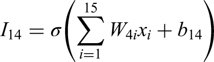

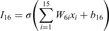
Combining it all into a matrix form, we can represent it as:
I = 
Similarly, for each layer in the neural network, the computations can be expressed as: Input layer, I = Hidden layer, H1 = Output, Y=
DNN Model
DNNs are capable of capturing more complex patterns in data due to the increased number of processing steps. The traditional methods require hand-crafted feature extraction, whereas DNNs can automatically learn the most relevant features from the data itself. This helps in reducing human bias and streamlines the analysis process.
Our proposed DNN model architecture has a first layer of input, three hidden layers, and an output layer. Each layer consists of 78, 32, 16, 8, and 1 neurons, respectively. The choice of pyramidal network design is made as it progressively distils the input features. 58 All the layers except the output layer use the ReLu activation function. The output layer uses the sigmoid activation function. All the layers are fully connected (FC). A dropout of 0.5 and 0.3 is done in the first dense layer and first hidden layer, respectively. Dropout is a regularisation technique where randomly selected neurons are ignored during the training process in order to prevent overfitting due to interdependence among neurons. Figure 4 shows the five-layer architecture of the DNN model. All the input features are scaled before being directly fed into the DNN as inputs. We performed hyperparameter optimisation using both grid search and random search strategies. The search space included variations in activation functions (ReLU and sigmoid), optimiser choices ('sgd’, ‘adam’, ‘rmsprop’, ‘nadam’), batch sizes (16, 24, 32, 64), learning rates (0.001 to 0.01), and dropout (0.1 to 0.5). During random search, we performed 50 iterations, randomly sampling the number of hidden layers (ranging from 1 to 5), and the range for number of neurons was given as ([64, 78, 85, 90], [16, 32, 40, 48], [8, 16, 24], [4, 8, 12], [1, 2, 4]). For the number of epochs, we implemented early stopping and selected the optimal epoch based on the best validation performance recorded in the training history. The chosen hyperparameters for DNN include a learning rate of 0.001, a batch size of 24, an optimiser of Adam, and epochs of 15.

Architecture of the DNN model.
Combining all the input from individual neurons in the input layer into a matrix form, we can represent it as:
Similarly, for each layer in the neural network, the computations can be expressed as:
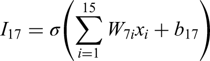
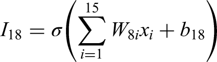
Input layer, I = First hidden layer, H1 = Second hidden layer, H2 = Third hidden layer, H3 = Output, Y =
σi indicates ReLU activation function for i<=4, and σ5 indicates sigmoid function. The variable xi refers to the ith input feature and Wji denotes the weight associated with neuron j against the input feature xi and Wk denotes the weight matrix at kth layer. Similarly, the variable bkj denotes the bias term at jth neuron at the kth layer and Bk indicates the bias matrix at the kth layer. The variable Ikj represents the total input at jth neuron at the kth layer, and I represents the output of the first layer. Hk denotes the output of the kth hidden layer. Y represents the final output obtained from the DNN.
Results
In this section, we evaluate the performance of the models developed and present the results. Then, based on the observed results, we explain and interpret the model outcomes. Followed by the development of the ensemble model and the evaluation of its performance.
Cross Validation
In situations where the available dataset is limited, cross-validation ensures reliable evaluation by using different subsets of available data for training and testing in multiple folds, making it less likely that the model will perform well solely due to chance. 60 We use a 10-fold cross-validation to evaluate the performance of our model. Precision and recall are crucial metrics in the context of medical applications, where the false positives (FP) and false negatives (FN) can have significant impacts on patient outcomes. Precision indicates the accuracy of positive classifications. In cancer diagnosis, high precision means that when the model classifies a case as malignant, it is likely to be correct. High recall suggests a lower risk of FN, which is critical in cancer diagnosis, as a missed malignant case can delay the treatment. A good F1-score indicates a better balance between precision and recall. The receiver operating characteristics-area under the curve (ROC-AUC) provides a comprehensive summary of a model's performance 61 across various classification thresholds. It considers the trade-off between true positive rate (TPR) and true negative rate (TNR). Table 3 compares the performance of the candidate models developed. It can be observed that the DNN model, which used all the 78 attributes, scored higher accuracy, recall and F1-score than the simple ANN model. The simple ANN model, which used only 15 relevant attributes, scored higher precision than the DNN model.
Performance Metrics for the ANN and DNN Models.
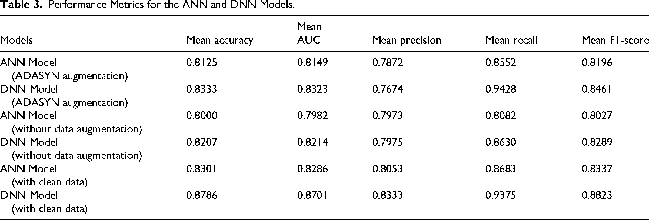
From Table 3, it can be observed that with clean data (without rare records), the performance of the DNN model is very good, and the ANN model performs slightly inferior. However, in the medical domain, it makes sense to consider rare medical cases while developing the model. A model trained without considering rare cases might become biased towards more common conditions, reducing its generalizability and reliability when deployed in clinical settings. The ADASYN augmented data yielded better results for our models than the data without augmentation. Hence, we choose to develop fair models that offer inclusivity to diagnose rare medical conditions. We then tried to enhance the diagnosis performance of these models through additional steps.
Calibration Curve
A calibration graph gives a visual representation of the quality of model suitability by illustrating the observed values and true values in the evaluation. It is commonly used in ML to assess the rightness and reliability of the model classifications. 62 Calibration graphs are important tools in evaluating ANN and DNN models because they provide insight into the reliability and accuracy of the model's predictions. The x-axis of the graph typically represents the predicted probabilities generated by the model, while the y-axis represents the actual observed outcomes.63,64 By comparing these values, we can assess how well the model's classification aligns with the actual underlying probabilities. In a well-calibrated model, the points on the calibration graph should fall along a diagonal line, indicating that the predicted probabilities closely match the true probabilities. Deviations from the diagonal line suggest calibration errors, indicating that the model's predicted probabilities may not accurately reflect the true likelihood of events. Platt scaling is a method used to calibrate the output probabilities. 62 It involves fitting a logistic regression model to the predicted probabilities to map them to calibrated probabilities.
Figure 5 compares the calibration curves, plotted with Platt scaling, for the ANN and DNN models. From the graphs, it can be observed that the ANN exhibits a better orientation to the ideal calibration curve than the DNN model for higher prediction probabilities. This could be because DNNs require large datasets to leverage their capacity effectively, which is not the case here. When the dataset is small or noisy, ANNs, being simpler, may perform better as they don't overfit as easily.

Calibration Curves of ANN and DNN Models.
Error Analysis
We performed an error analysis augmented with counterfactual reasoning on how minimal changes to those features could potentially correct the model's errors. We identified misclassified samples by comparing predicted labels to true labels on the test set. The percentages of true positives are 43.06%, false positives are 9.03%, true negatives are 43.06%, and false negatives are 4.86%.
Among the false positives and false negatives, we selected representative samples for deeper interpretability. To explain misclassified predictions, we used the diverse counterfactual explanations (DiCE). 65 For each misclassified instance, we generated multiple diverse and plausible counterfactuals and observed a minimum change in a set of impactful features that can flip the decision right.
Table 4 shows the top features identified by DiCE that are sufficiently perturbed in order to change the model's output from a false positive to a true negative diagnosis. Average reductions in these identified features sufficient for the model to flip the decision from cancer to no cancer are shown.
Counterfactual Explanation for False Positives to True Negatives Using DiCE.

Table 5 shows the top features identified by DiCE that are sufficiently perturbed in order to change the model's output from a false negative to a true positive diagnosis. Average reductions in these identified features sufficient for the model to flip the decision from no cancer to cancer are shown. These observation shows the major factors that confuse the diagnosis model to misclassify the cases.
Counterfactual Explanation for False Negatives to True Positives Using DiCE.

Explaining Model Decision
Explaining and interpreting the results of neural network models may be crucial for building trust, providing transparency, accountability, and error diagnosis. Interpretation of the models presents the details of the methods and techniques used in the models to arrive at the decisions. SHAP and LIME are two popular methods that can explain neural network classifications. LIME focuses only on local interpretability based on the instances, whereas, SHAP offers both local and global interpretability, consistent interpretations based on SHAP values. Though SHAP is computationally intensive and complex, it is a more accurate and theoretically sound explanation than LIME interpretations.24,64 Hence, we use the SHAP tool to interpret our models.
For a binary classification model, the SHAP value for feature i is computed using the equation (1)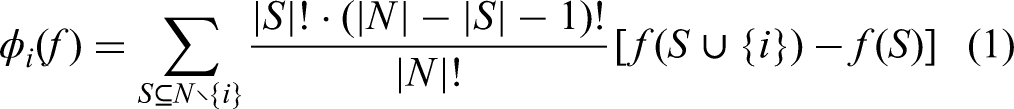
Where
Positive SHAP values indicate that the feature contributes positively to the decision, while negative SHAP values indicate a negative contribution. Features with larger absolute SHAP values are considered more important in influencing the model's decisions. 64 Figure 6 shows the 3D visualisation of the SHAP values for a subset of medical instances and their corresponding features. The red scale corresponds to a positive diagnosis, whereas the blue scale corresponds to a negative diagnosis. The final decision for an instance can be interpreted as a function of the sum of individual SHAP values for each feature.
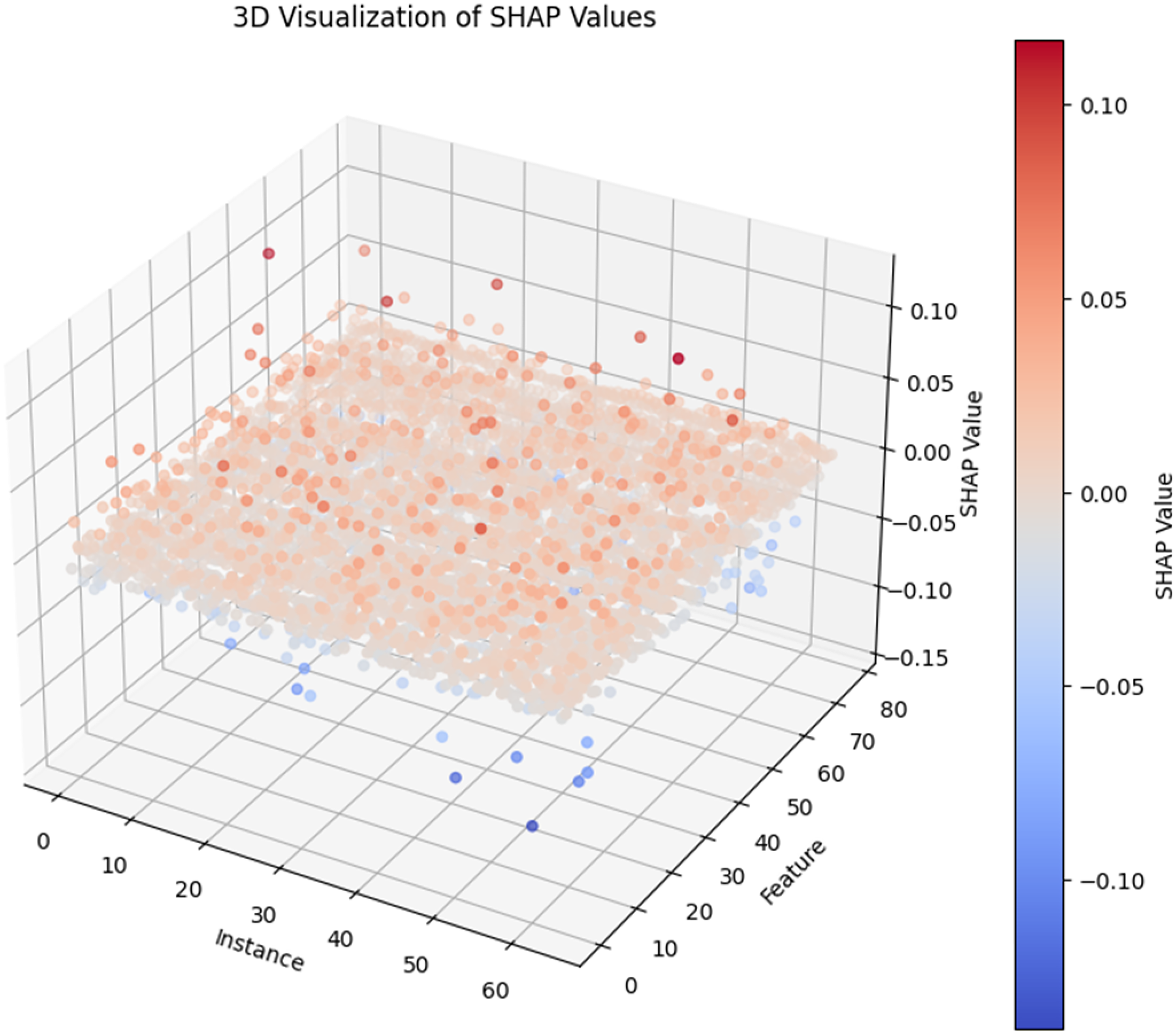
The 3D visualisation of SHAP values.
Explaining the ANN Model Outcome Using SHAP Interpretation
Figure 7 shows the top fifteen features contributing to the model's decision, ranked in descending order. We can identify Hemoglobin, ESR and Neutrophils as the top features that contribute to the lung cancer diagnosis. The left or right orientation of the colour scale indicates the direction of impact of the model for a change in feature value. For example, the red points of ESR are on the positive SHAP scale, which indicates that high ESR contributes positively to lung cancer diagnosis and low ESR contributes negatively. Meanwhile, the attribute RBC is vice versa due to the opposite direction of colouring. From Figure 7, all features except Pneumonia and RBC contribute positively to lung cancer diagnosis.

SHAP Summary Plot for the ANN Model.
Figure 8 shows the mean absolute SHAP values of each feature based on the class. This represents the average impact each feature has in labelling an instance to a particular class by the ANN model. For instance, the red bar represents the impact of each feature contributing to labelling a case as malignant. To further understand the associations between features and their contribution to lung cancer diagnosis, we plot dependency graphs. The dependency plot has SHAP values of a feature on the y-axis and standardised values of that feature on the x-axis. The colour gradient represents its association with another feature.
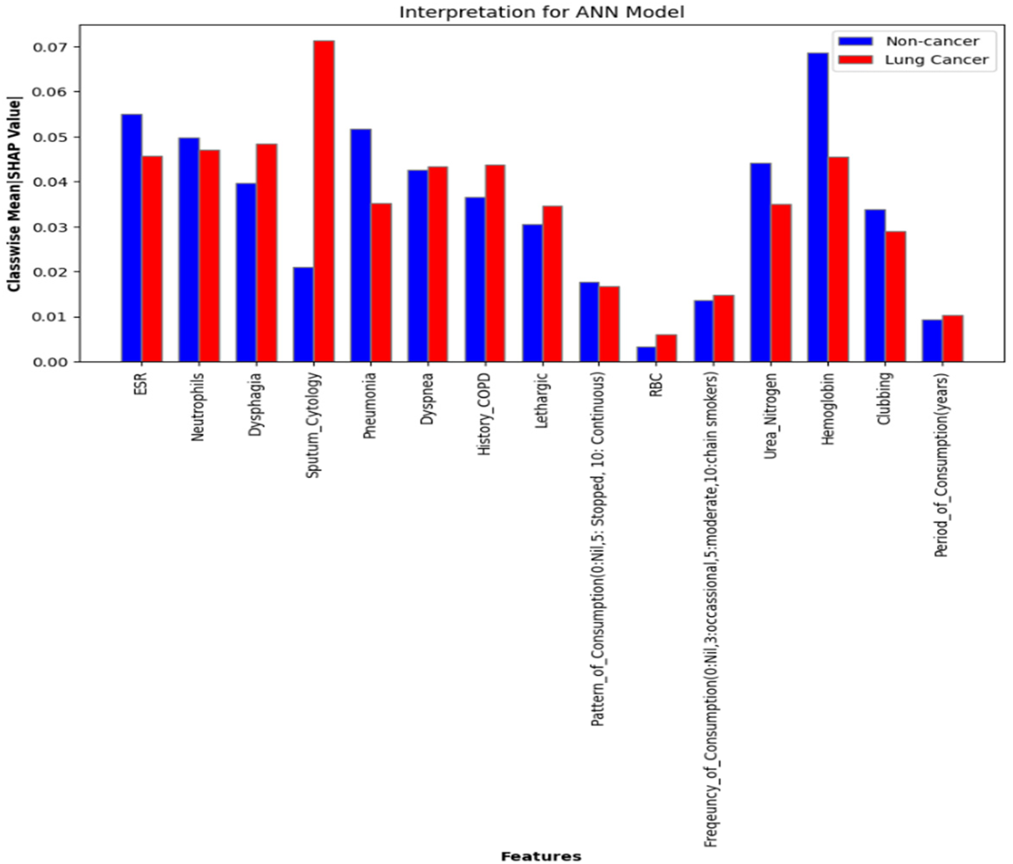
Classwise mean absolute SHAP values for the ANN model.
Figure 9 shows the two dependency plots for ESR against a period of consumption (tobacco) and frequency of consumption (tobacco) of the ANN model. Two noteworthy associations were made while exploring the dependencies of features using SHAP values. There is an increasing tendency in patients with higher periods of tobacco consumption and higher frequency of consumption to have increased ESR values. This insight aligns with the relevant clinical literature.66–68 In addition, a higher ESR value has a higher SHAP value, which indicates increased chances of a lung cancer diagnosis.

SHAP Dependency Plot of the ANN Model.
Explaining the DNN Model Outcome Using SHAP Interpretation
Figure 10 shows the SHAP summary plot for the DNN model. It contains the top 20 features that significantly contribute to lung cancer diagnosis by the DNN model based on their corresponding ranking. The three most significant features of this model are ESR, Mode_of_Tobacco, and Sputum_Cytology. From Figure 10, all the features except History_Respiratory_Tract_Infection, Lymphs, Fever, Platelets, and Spirometry contribute positively to the lung cancer diagnosis.

SHAP summary plot for DNN model.
Figure 11 shows the mean absolute SHAP values of each feature based on the class. This represents the average impact each feature has in labelling an instance to a particular class by the DNN model. For example, the red bar against the feature Sputum_Cytology shows its huge impact in labelling a case as malignant with a mean absolute SHAP value above 0.025. Its impact on labelling a case as non-cancerous is relatively less. Further associations of these primary features are visualised as dependency graphs, as shown in Figure 12. These results are then reviewed by domain experts to ensure their clinical relevance.
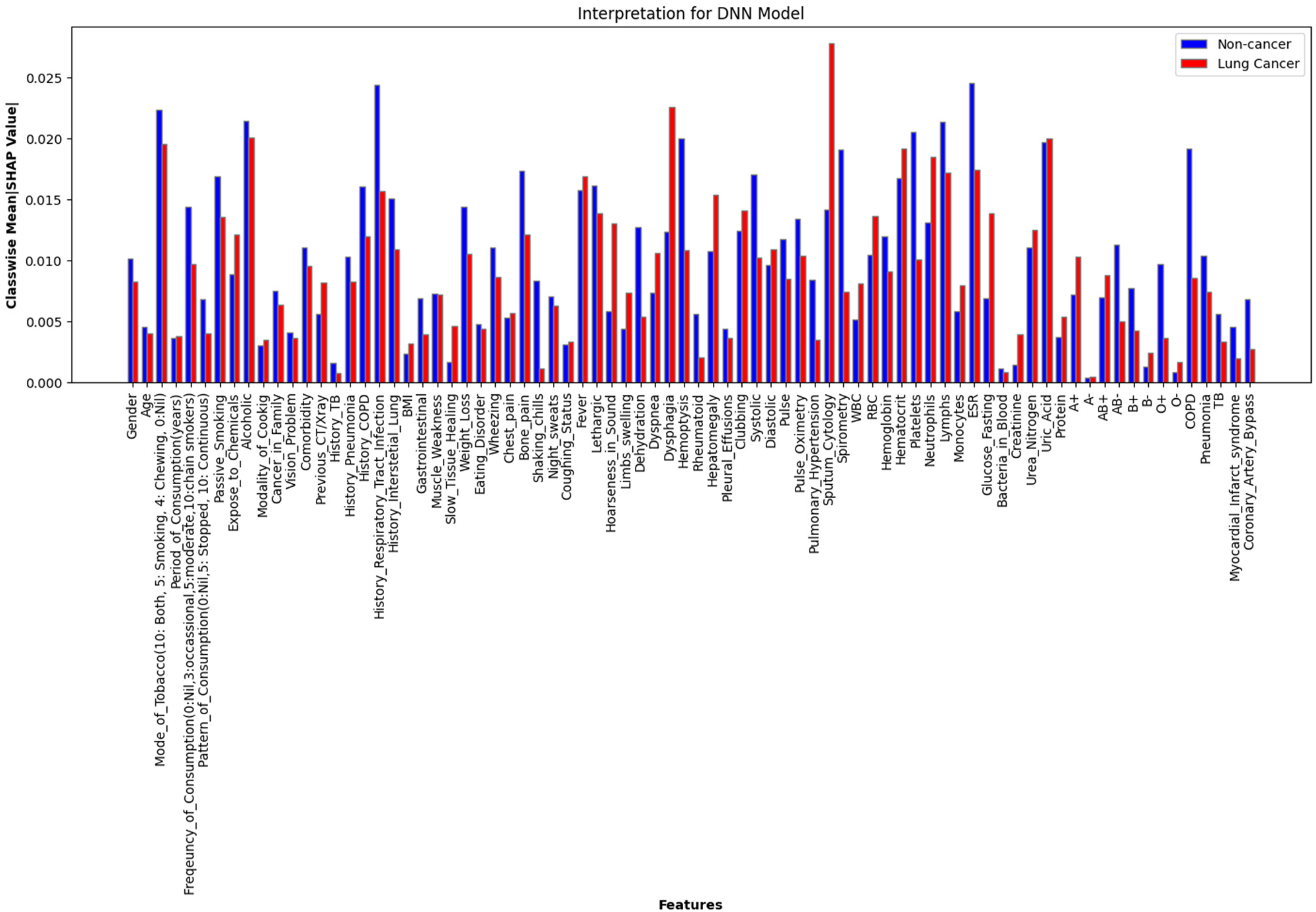
Class-Wise Mean Absolute SHAP Values for the DNN Model.

SHAP dependency plot of the DNN model.
Figure 12 shows the dependency graphs plotted for the features of the DNN model. The first two dependency plots align with the findings in the dependency plots for the ANN model. The third dependency plot indicates an association of high Hoarseness_in_Sound to the severity of Coughing_Status, both of which contribute positively to the malignancy diagnosis. The fourth dependency graph shows the increasing tendency of association of high ESR values with high History_of_COPD. The fifth dependency graph indicates that the occurrence of COPD has a high association with low Pulse_Oximetry. The sixth dependency graph shows that pleural effusions are associated with lower values of Pulse_Oximetry.
In our ANN model with fewer features, the model relies more heavily on each feature, and so their SHAP values are typically higher. In the DNN model, which has many features, the model might still rely on significant features, but the SHAP values tend to be lower because the contributions are spread out across more features. Hence, the importance is distributed across a larger number of features, leading to smaller individual SHAP values. As a result, the threshold of significance can vary for each case based on the relative ranking. One interesting observation in the interpretation of the diagnosis models developed is that the attribute ESR is a major determinant that favours a malignancy diagnosis in both models. This indicates that an elevated ESR value is a prominent factor in labelling a patient's case as malignant, but it is not a sufficient condition, ie, a high ESR does not necessarily imply the presence of cancer. However, elevated ESR levels were observed in a larger proportion of lung cancer patients.
Developing an Ensemble Model
Now we have two models, one with better accuracy and recall (DNN model) and the other with better precision and calibration (ANN model). We utilise the benefits of the individual models and mitigate the effect of biases by leveraging an ensemble model for diagnosis using two approaches. The weighted voting ensemble approach directly combines predictions of individual models using predefined weights.
69
This approach does not involve training a meta-model on top of the base model predictions. The final output is computed using equation (2).
Where,
On the other hand, the stacking ensemble approach involves training base models (ANN and DNN models) and then using their predictions as inputs to a meta-model (logistic regression) that makes the final decision.
70
The final output of the models is computed using equation (3).
Where,
Figure 13 shows the AUC scores of the Weighted voting ensemble model and the stacking ensemble model. For instance, the weighted voting with ANN model weight 0.4 and DNN model weight 0.6 yielded a mean AUC of 0.85, and the Stacking approach yielded a mean AUC of 0.86.

AUC Scores of the Weighted Voting Ensemble Model and the Stacking Ensemble Model.
It can be observed that the Stacking ensemble approach has improved the overall diagnosis capability of the model despite having rare record data. It achieved a performance comparable to that of the DNN model with clean data. The stacking ensemble model gives a mean accuracy of 0.8558, a mean AUC score of 0.8600, 0.8092 mean precision, 0.9282 mean recall, and 0.8646 mean F1-score. These performance scores are satisfactory for developing practical models. The Weighted ensemble model is giving a mean accuracy of 0.8411, a mean AUC of 0.8500, 0.7846 mean precision, 0.8907 mean recall, and a mean score of 0.8342. Figure 14 shows the model accuracy comparison with 95% confidence interval (C.I.). The error bars do not overlap with those of the ensemble model, indicating its statistically significant superior performance.

Model accuracy comparison with 95% C.I.
Discussion
Given the moderate sample size and high dimensionality, we are aware of the high risk of overfitting for the DNN model; however, we took several rigorous steps to mitigate this by employing cross-validation and dropout. We also kept the network architecture intentionally shallow and limited the number of parameters to suit the small dataset size.
Overfitting would be indicated by the increased difference between average validation loss and average training loss. From Figure 15, we do not observe any signs of relevant overfitting. Having addressed that concern, we now turn our attention to two key aspects of this research: the use of ADASYN and the implementation of an ensemble model.

Training Versus Validation Loss for DNN Model.
ADASYN is employed to address the challenge of class imbalance in medical datasets, particularly when rare conditions are underrepresented. This approach is crucial to ensure fairness in medical research, where certain disease conditions may have limited data due to their rarity. The possible biases can be mitigated carefully through expert review of the generated synthetic samples and regularisation. Thereby ensuring proper management of the potential drawbacks. This inclusivity is vital for developing diagnostic tools that perform equitably across diverse patient populations, preventing the neglect of rare cancer cases.71,72
The benefit of the ensemble model can be leveraged when the base models have diversity in their operation, when the individual models are learning and making different kinds of errors. Here, our ANN model has increased precision, and the DNN model has increased recall; therefore, the ensemble facilitated the imbibe the merits of both models. Since the data size is limited, adding more base models might result in overfitting. Also, if the errors of the base models are not complementary, adding additional models will not benefit to the ensemble performance. Youden's J statistic can be used to find the optimal threshold for classifying the classes to avoid a high disparity between accuracy and AUC values for the model. For our final model, the optimal threshold for classification is 0.3936. The ensemble model with a stacking approach can give a better performance with the dataset containing rare outlier data, which is comparable to the performance of the DNN model trained on clean clinical data. We evaluated the statistical significance of the performance differences between the ensemble model and the DNN model (trained on clean data) using McNemar's test. 73 The resulting test statistic was 0.2500 with a p-value of 0.6171, indicating no statistically significant difference between the two models. In contrast, when comparing the ensemble model with the DNN model trained on ADASYN-augmented data, the test yielded a statistic of 107.6412 with a p-value of 0.0000, indicating a statistically significant improvement in performance by the ensemble model.
Comparing the Proposed Model with the Latest Models
In this section, we compare the performance and features of the proposed model to the latest models developed for lung cancer diagnosis, prediction, and prognosis. Table 6 highlights the key advantages of the proposed model. It is explainable, poses no health risks as it relies solely on routine clinical data without the need for repeated radiomic procedures, and is cost-effective since it does not require sophisticated tests or complex processing. Additionally, the model is scalable and can be deployed across a wider range of medical centres, unlike the models that use advanced technologies based on genomic data, which are often accessible only to a privileged segment of the population. Notably, this model has been developed to include rare cases of lung cancer, ensuring fairness and inclusivity in its application.
Comparison of Model Features of the Proposed Lung Cancer Diagnosis Model with the Latest Lung Cancer Models.

Table 7 presents the approximate cost range associated with various diagnostic methods. Among all the services, clinical evaluation emerges as the most cost-effective option on average.76,77
Approximate Cost Range for Different Medical Services.

Several recent studies have raised safety concerns by reporting cases of radiation-induced cancer.78–80 Though LDCT is not expensive and widely accessible, it will not provide adequate images in obese patients. Heavier patients receive higher doses of radiation. Our proposed diagnostic model does not rely on radiomic features or imaging-based data. Instead, it utilises routine clinical data, making it a significantly safer and more cost-effective alternative.
Limitations
However, given the limited scale of the dataset used in this research, we propose this study as a prototypical research cohort for the development of a clinical data-based lung cancer diagnostic system. In its current form, the proposed model is best suited as a pre-screening tool rather than a definitive lung cancer diagnostic solution. With training on larger and more diverse datasets, the model has the potential to achieve improved generalizability and more precise factor identification, at which point it could serve as a robust tool for lung cancer diagnosis.
Implications of Excluding Rare Medical Records from Training Data
The scope of applicability of the model trained without considering rare cases becomes limited, as it fails to recognise and handle the full spectrum of possible conditions, including rare but critical ones. Failing to account for rare cases can lead to inequitable healthcare services. Misdiagnosis or delayed diagnosis of rare conditions can lead to incorrect treatments, which can undermine patients’ health and increase costs. Also, over the years, medical practitioners may become overly reliant on the model, leading to a lack of awareness and knowledge about rare conditions. Hence, the models need to learn from properly handled rare medical records.
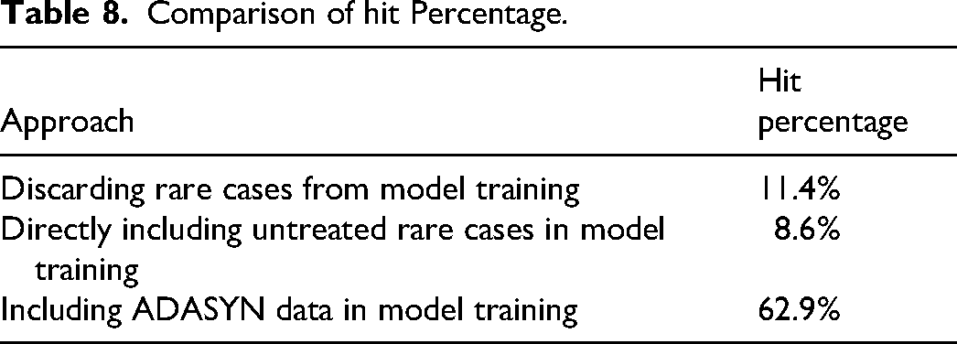
Table 8 highlights the clear advantage of using ADASYN augmentation for improving the diagnosis of rare cases. From a set of 35 actual rare case records, our approach achieved the highest number of correct diagnoses, demonstrating its effectiveness in addressing data imbalance in medical applications.
Comparison of hit Percentage.
Implications of XAI
Explainability in neural network-based models for lung cancer diagnosis has significant implications for various stakeholders such as doctors, patients, researchers, and regulatory bodies. It increases the trust among doctors by providing insights into the decision-making process, which is crucial for adopting AI models in clinical practice. From the SHAP interpretations, we can observe that the significance and impact of each clinical symptom in deciding a particular class has a large variance. These variations and insights are hard to comprehend by human cognitive skills, despite having years of clinical experience. Therefore, the explainable models not only give a proper diagnosis but also serve as a robust quantitative explanation of how the diagnosis model labels a patient case. The clear explanations of the model also allow doctors and researchers to identify potential flaws or biases in the model, leading to the development of more accurate and reliable diagnostic tools. Understanding the model will guide iterative improvements, which can guarantee that the AI model will remain accurate and relevant as and when new data arrives. Patients will be more open to AI-based interventions without anxiety.
Financial Implications
The proposed XAI model for lung cancer diagnosis can be easily deployed into the clinical setup as it does not incur a huge capital investment in buying any hefty diagnostic equipment. The only additional cost associated with implementing this AI model in practice is to provide training for medical practitioners. This involves teaching them how to collect high-quality clinical data, run the model with proper interfaces and understand the model's decisions based on the interpretations.
Conclusion
Alternative techniques for radiation-based screening to diagnose lung cancer are in high demand due to the increased rate of late-stage diagnoses and associated exposure risks. Although several novel alternatives have been developed, their widespread adoption is hindered by high costs and limited access to necessary resources. 5 Leveraging clinical data presents a cost-effective and viable solution to this problem. Often, early clinical indications of lung cancer are overlooked or considered insignificant, contributing to delays in diagnosis. A key strength of the proposed approach lies in its seamless integration with existing clinical workflows, requiring no additional investment in equipment or diagnostic procedures. By utilising routinely collected clinical data, our tool provides a resource-efficient method for identifying patients at risk of lung cancer, significantly reducing operational costs.
This research presents an XAI model for the early diagnosis of lung cancer using clinical data. The model emphasises accurate diagnosis along with interpretability, aiming to build trust among healthcare practitioners and patients. One major challenge in building a diagnostic model from clinical data is handling missing values. Given the prevalence of non-Gaussian data distributions, the semiparametric MICE method was employed to impute missing values effectively. Two XAI models were developed. The ANN model uses 15 selected, clinically relevant features, while the DNN model incorporates 78 features to capture complex patterns in the data. ADASYN augmentation was applied to address the imbalance caused by rare medical records. The DNN model demonstrated superior performance in terms of accuracy, AUC, and recall. In contrast, the ANN model showed better precision and calibration when trained with ADASYN-augmented data.
Another significant barrier to the adoption of AI in clinical settings is the lack of interpretability. Healthcare professionals are often presented with black-box decisions, making them reluctant to trust or endorse such models. This paper addresses this issue using SHAP for global interpretation. Both models’ decisions are explained using SHAP, providing transparency into their diagnostic rationale. To capitalise on the strengths of both models, we developed a stacking ensemble that yielded diagnostic performance comparable to the DNN model trained on clean data, while improving robustness.
In a clinical workflow, patient observations can be input into the model to generate a diagnosis that is either positive or negative. These models can be continuously updated with new clinical data, enhancing their accuracy and effectiveness over time. Medical practitioners require minimal training to operate the model and can easily interpret its outputs. The combination of affordability, accessibility, and interpretability makes our XAI models a promising and safe alternative to traditional radiation-based screening for early lung cancer diagnosis. Additionally, the model must comply with relevant regulatory standards. 81 This includes obtaining regulatory approvals such as those required for Software as a Medical Device or under the European Union Medical Device Regulation, adhering to artificial intelligence-specific guidelines like the Food and Drug Administration's Good Machine Learning Practices and the International Organization for Standardization Technical Report 24028, as well as ensuring compliance with data privacy regulations such as the Health Insurance Portability and Accountability Act and the General Data Protection Regulation.
However, the current XAI models are trained on a relatively limited dataset, which constrains their reliability and generalizability as fully assertive diagnostic tools. At this stage, the model should be regarded as a prototype and a feasibility study. Our findings aim to support healthcare practitioners in adopting a cost-effective, interpretable pre-screening tool for identifying high-risk lung cancer patients.
Future Work Should Focus on Several key Areas:
Dataset expansion and diversity: To enhance model robustness and applicability, future research should involve training and validating the model on larger, multi-institutional datasets that include a more diverse patient population across different age groups, ethnicities, and geographic regions.
Improvement of data augmentation techniques: While ADASYN has proven effective in our research, its performance can be further optimised. Future work could explore hybrid augmentation strategies combining ADASYN with generative models to create more realistic synthetic samples and avoid overfitting.
Model calibration and reliability: Calibration of deep learning models remains a critical step to ensure that predicted probabilities reflect true risks. Techniques such as temperature scaling, isotonic regression, or Bayesian deep learning approaches could be considered to enhance the trustworthiness of predictions, especially in clinical settings.
Clinical validation and deployment: Real-world testing through prospective clinical trials is essential to validate the utility and impact of the model in actual healthcare environments. Integration with existing diagnostic workflows and evaluation of cost-effectiveness, decision impact, and clinician trust will be crucial steps toward clinical deployment.
By addressing these areas, future iterations of our model can move closer to deployment as a reliable, generalizable, and interpretable decision-support tool for early lung cancer detection.
Footnotes
Ethics Statement
This research is conducted by a collaborative team of technical and medical experts of the field in line with the ethical and data collection standards outlined in [ 45 ]. This research was approved by the institutional ethics committee of Government Medical College, Kozhikode, and adhered to their de-identification protocols. Reference no. GMCKKD/RP 2019/IEC/148.
Funding
The authors received no financial support for the research, authorship, and/or publication of this article.
Declaration of Conflicting Interests
The authors declared no potential conflicts of interest with respect to the research, authorship, and/or publication of this article.