Sage Journals: Discover world-class research

Abstract

Introduction: The application of single-cell RNA sequencing to delineate tissue heterogeneity and complexity has become increasingly popular. Given its tremendous resolution and high-dimensional capacity for in-depth investigation, single-cell RNA sequencing offers an unprecedented research power. Although some popular software packages are available for single-cell RNA sequencing data analysis and visualization, it is still a big challenge for their usage, as they provide only a command-line interface and require significant level of bioinformatics skills. Methods: We have developed scAnalyzeR, which is a single-cell RNA sequencing analysis pipeline with an interactive and user-friendly graphical interface for analyzing and visualizing single-cell RNA sequencing data. It accepts single-cell RNA sequencing data from various technology platforms and different model organisms (human and mouse) and allows flexibility in input file format. It provides functionalities for data preprocessing, quality control, basic summary statistics, dimension reduction, unsupervised clustering, differential gene expression, gene set enrichment analysis, correlation analysis, pseudotime cell trajectory inference, and various visualization plots. It also provides default parameters for easy usage and allows a wide range of flexibility and optimization by accepting user-defined options. It has been developed as a docker image that can be run in any docker-supported environment including Linux, Mac, and Windows, without installing any dependencies. Results: We compared the performance of scAnalyzeR with 2 other graphical tools that are popular for analyzing single-cell RNA sequencing data. The comparison was based on the comprehensiveness of functionalities, ease of usage and flexibility, and execution time. In general, scAnalyzeR outperformed the other tested counterparts in various aspects, demonstrating its superior overall performance. To illustrate the usefulness of scAnalyzeR in cancer research, we have analyzed the in-house liver cancer single-cell RNA sequencing dataset. Liver cancer tumor cells were revealed to have multiple subpopulations with distinctive gene expression signatures. Conclusion: scAnalyzeR has comprehensive functionalities and demonstrated usability. We anticipate more functionalities to be adopted in the future development.

Keywords

single-cell RNA-seq data analysis software liver cancer tumor heterogeneity

Introduction

Single-cell RNA sequencing (scRNA-seq) is different from the conventional bulk-cell sequencing approach. It can effectively investigate cellular heterogeneity.¹ It can be used to study developmental processes and pathological mechanism of diseases.^2,3 In addition, scRNA-seq can discover complex and rare cell populations,⁴ track the trajectories of distinct cell lineages in developmental stages,⁵ and reveal regulatory relationships between genes.⁶ Importantly, it can lead us to discover the previously uncovered cell populations and suggest how distinct subpopulations of cells respond to disease progressions.⁷ Regarding liver cancer, it is known to have a high degree of intra-tumoral heterogeneity,^8,9 and therefore, scRNA-seq is an ideal tool to perform its cellular and molecular investigations.¹⁰ A range of software tools and packages (https://www.scrna-tools.org/) are available for scRNA-seq data analysis. The majority of them are command-line, without a graphical user interface. Popular command-line analysis packages are Seurat,⁴ Scater,¹¹ and Scanpy.¹² Only very few tools have been developed with graphical user interface, such as ASAP,¹³ Granatum,¹⁴ and SINCERA.¹⁵ However, they have limited functionalities on restricted perspectives (some of them have only visualization function¹⁶) and may not support the whole course of scRNA-seq data analysis. Moreover, they may not have enough user-defined parameters that allow for flexibility, and some of them cannot handle large dataset.

To alleviate the aforementioned research gaps, we developed scAnalyzeR (scRNA-seq Analyzer), which provides a wide range of functionalities with an interactive graphical user interface for analyzing scRNA-seq data. It covers a comprehensive workflow including dataset uploading, data preprocessing (discarding low-quality samples, and outlier detection and removal), normalization, highly variable gene (HVG) identification, cell clustering, differential gene expression analysis, data visualization (dimension reduction plot, violin plot, feature plot, heatmap, dynamic principal component analysis [PCA] plot, and correlation plot), pathway enrichment analysis, and pseudotime trajectory construction. Moreover, scAnalyzeR is completely dockerized,^17,18 thus users will not be required to install any dependencies. It also allows users to analyze large-scale scRNA-seq datasets.

In this study, we developed our comprehensive scRNA-seq analysis tool and compared its performance with other scRNA-seq analysis pipelines with graphical interface. The comparison of scAnalyzeR and the other tools was in terms of comprehensiveness of functionalities, ease of usage and flexibility, and execution time. To illustrate the usefulness of scAnalyzeR in cancer research, we analyzed our in-house liver cancer scRNA-seq dataset. Intriguingly, tumor cells stratified according to multiple liver cancer stem cell (CSC) marker expressions.

Materials and Methods

Implementation of scAnalyzeR

The overall workflow of the scAnalyzeR is divided into 9 primary modules, as depicted in Figure 1: (i) upload dataset, (ii) preprocessing, (iii) normalization, (iv) dimensionality reduction, (v) clustering, (vi) differential expression (DE), (vii) plots, (viii) pathway analysis, and (ix) trajectory analysis. The scAnalyzeR was developed using Shiny web framework¹⁹ with RStudio²⁰ and written in the statistical programming language R.²¹ It relied on some of the functionalities of Seurat⁴ and Monocle.⁵ For interactive designing of the user interface, the R package ShinyJS²² was used. Various R packages were also used as dependencies, including DT²² for output data table formation and exhibition in different modules, plotly²³ for interactive dynamic graphs (eg, dynamic PCA plot), dplyr²⁴ for data manipulation, and ggplot2²⁵ for presenting bar plots.

Figure 1.

Workflow of the scAnalyzeR. Major steps include dataset uploading, preprocessing, data normalization, dimension reduction, clustering, differential expression analysis, data visualization, pathway analysis, and pseudotime trajectory analysis.

Comparison With Other Existing Tools

We compared the scAnalyzeR with other similar scRNA-seq analysis pipelines with graphical interface. In this comparison study, the scAnalyzeR was compared with Granatum¹⁴ and ASAP¹³ tools in terms of functionalities (Table 1), the number of parameters available, and the execution time using the 3 K peripheral blood mononuclear cells (PBMCs) dataset.

Table 1.

Comparison of Functionalities With Other Similar Existing Tools.

Functionalities		scAnalyzeR	Granatum	ASAP
Uploading	Delimited text file	√	√	√
Uploading	Cellranger output files (MEX)	√	×	×
Preprocessing		√	√	√
Normalization and Scaling		√	√	√
Highly variable genes (HVGs) selection		√	√	√
Imputation		×	√	×
Dimensionality reduction		√	√	√
Clustering		√	√	√
Differential expression (DE) analysis	Find all markers	√	√	√
	Cluster oriented markers	√	×	×
	Cluster combination	√	×	×
Gene set enrichment analysis (GSEA)		√	√	√
Protein network construction		×	√	×
Pseudotime construction		√	√	×
Pseudotemporal heatmap		√	×	×
Other plots		Heatmap, Violin plot, Dynamic PCA, and Correlation plot (between 2 genes)	×	×

Example Datasets for Implementation and Illustration of scAnalyzeR

To implement the scAnalyzeR, we used the example dataset of 2700 PBMC from 10X Genomics (referred as 3 K PBMC dataset thereafter) (https://support.10xgenomics.com/single-cell-gene-expression/datasets/1.1.0/pbmc3k) for testing and illustration purpose. To illustrate the application of scAnalyzeR in cancer research, we used the previously published²⁶ in-house scRNA-seq dataset (13,789 genes across 139 tumor cells that were derived from a patient-derived tumor xenograft model established from hepatocellular carcinoma (HCC) patient.

Results

Illustration of scAnalyzeR

User interface

The scAnalyzeR provides a comprehensive graphical user interface for analyzing and visualizing scRNA-seq data. The user can visit the individual analysis module simply by clicking the different analysis tabs. Default parameters are provided but users can make any necessary changes. Besides, figures and output data tables can be downloaded.

Upload dataset

The scAnalyzeR accepts either a delimited text file (containing the gene expression matrix for cells) or Cell Ranger output files (barcodes, genes, and matrix file) as an input. The user is required to choose an appropriate species (human or mouse) option before uploading the data file. A text notification will be shown automatically after uploading the data file successfully. For illustration purposes, plots were generated using 3 K (2700 single cells with 32,738 genes) PBMC dataset from 10× Genomics (https://support.10xgenomics.com/ single-cell-gene-expression/datasets/1.1.0/pbmc3k).

Preprocessing

The scAnalyzeR provides a filtering process to detect outlier samples as well as to remove them. We performed preprocessing steps (Create dataset and Filtering) by default settings, and it can also be run with different parameters. In Create dataset step, the Minimum no. of cells (MCs) was set to 3, and Minimum no. of genes (MGs) was set to 200, and the created dataset remained with 13,714 genes across 2700 cells. The created dataset (before filtering) had the maximum number of features (number of genes expressed in a cell) around 3000, gene counts were approximately 15,000 and the mitochondrial percentage was nearly 20% (Figure S1A, C, E). The parameter settings in the Filtering step were as follows: nFeature_RNA > 200, nFeature_RNA < 2500, and percent.mt < 5%. The filtered dataset remained with 13,714 genes across 2638 cells for downstream analysis (Figure S1B, D, F).

Normalization and scaling

There are 3 available normalization methods (Log Normalization, Centered log-ratio transformation, and Relative counts) in the current version of scAnalyzeR. We used default settings for normalizing to the filtered dataset, where the Log Normalization method was applied, and the scaling factor was set to 10,000. In total, 2000 HVGs were selected and only these genes were used in the downstream analyses whenever indicated as “Highly Variable Genes Only.” Figure S2A shows a feature plot where red dots indicate HVGs and black dots represent non-HVGs. The list of HVGs can be reported in table format as well as a downloadable file. By default, the top-10 HVGs are shown as a table in the scAnalyzeR's interface (Figure S2B).

Dimensionality reduction

The dimensional reduction technique applied to the normalized dataset reduced the data dimensionality, where the multidimensional data is converted to a 2D space. We calculated 20 principal components in the normalized dataset, where only the HVGs (2000 genes) were used. Figure S3A describes the PCA plot after applying the linear dimensionality reduction method. We considered the first 10 principal components (PCs) (PC1-PC10) for subsequent analyses (Figure S3B and C). The t-SNE plot was generated using the first 10 PCs (Figure S3D). Besides, the heatmap illustrates the primary sources of heterogeneity in the PC1-PC2 (Figure S3E and F).

Clustering

The clustering analysis was performed based on the first 10 PCs (PC1-PC10), where the resolution was set to 0.4, and the default clustering method (Louvain algorithm) was applied from 3 available clustering methods. The t-SNE plot illustrates the clustering result (Figure S4A), and the bar graph shows the number of cells in each cluster (Figure S4B). Increasing the resolution value generated more cell clusters (Figure S5). In general, setting the resolution value between 0.4 and 1.2 gives good results, where the dataset contains around 3000 cells (Figure S5).

Differential expression

Three different strategies of DE analysis were implemented in scAnalyzeR: (i) find DE genes for every cluster, compared to all remained clusters, (ii) find DE genes in a particular cluster, compared to the remained clusters, and (iii) identify DE genes, cluster(s) versus cluster(s). We applied the ‘wilcox’ method for identifying DE analysis for every cluster, that is, DE analysis strategy (i). Figure S6A shows the total number of DE genes (both positives and negatives) in each cluster, before filtering. To filter the DE genes, we used the default parameter settings, after filtering, it was identified a number of up- and downregulated genes in each cell group (Figure S6B and C). Cluster oriented (Figure S7) and cluster(s) versus cluster(s) (Figure S8) DE analysis techniques were also implemented in scAnalyzeR.

Cell type identification

For illustration purposes, the well-known immune cell markers (Table S1, Figure S9) were used for cell-type identification in the 3 K PBMC dataset. CD14 was expressed in cluster 1. CD79A and CD8A were expressed in clusters 3 and 4, respectively. Therefore, CD14 + Monocytes (cluster 1), B Cell (cluster 3), and CD8 + T Cell (cluster 4) were identified in the dataset. CD3E was highly expressed in clusters 0, 2, and 6. These clusters were likely to be T cells. The CD68 marker was expressed highly in clusters 5, 7, and 8, which indicates their identity as macrophage. Collectively, distinct cell types were assigned to different cell clusters based on known immune cell markers (Table S2, Figure S10).

Plots

Other plotting functions were implemented in scAnalyzeR, namely, Heatmap (Figure S9A), Violin plot (Figure S9B), Feature plot (Figure S9C), Dynamic PCA plot (Figure S11), and Correlation plot (Figure S12). The Dynamic PCA provides a PCA plot for a given set of genes with some dynamic features. For instance, we calculated PCs for 45 genes across 2638 cells, and the computed result was illustrated on a 2D scatter plot (with PC1 and PC2) with several dynamic properties, such as zooming, rectangular selection, and lasso selection (Figure S11). Besides, to calculate the correlation between the 2 genes, a function was implemented in the Correlation Plot submodule, for example, the correlation between NKG7 and LTB genes (Figure S12).

Pathway analysis

DE genes were selected for GSEA, and either KEGG pathways or gene ontology terms can be used as the source of gene sets. The full list of the pathway result was available with necessary filtering when the GSEA computation was completed, and the user can download the GSEA results as well. The bubble plots showed the top 10 pathways (based on adjusted P value, ascending order) for both upregulation and downregulation (Figure S13A and B), separately. Moreover, the user can see either the list of significant or all gene sets (with gene symbol) in a particular pathway and visualize the heatmap plot for exploring the expression pattern for the selected pathway (Figure S13C and D).

Trajectory analysis

Pseudotime trajectory analysis module was implemented in scAnalyzeR for reordering cells based on the pseudotime. For trajectory analysis, either HVGs or all genes can be used as the input. In our analysis, the HVGs were used both in cell trajectory plots and pseudotemporal heatmap analysis (Figure S14).

Performance Comparison With Other Similar Tools

The comparison study among 3 distinct tools (scAnalyzeR, Granatum, and ASAP) was done based on the functionalities, execution time, and the number of parameters. Regarding functionalities, all 3 tools provided essential functionalities for scRNA-seq analyses. However, there were some differences (Table 2). scAnalyzeR implemented 14 out of 16 functionalities compared, except imputation, and protein network construction. On the other hand, 11 and 8 functionalities were implemented in Granatum and ASAP, respectively. Notably, imputation and protein network construction functions were only implemented in Granatum, but both of them failed to execute during the testing. In fact, Granatum could only execute the initial analysis parts (uploading, preprocessing, normalization, HVGs selection, dimensionality reduction, and clustering), and all the remaining steps failed to execute. In addition, all the cell clusters were labeled with the same color, but it was not clear to see for the overlapping cell groups (clusters), although cells were labeled with cluster number (Figure S15). Besides, scAnalyzeR provided several unique functionalities, including accepting Cellranger output files as input, different ways to define groupings for DE analysis, as well as various analysis plots, for example, heatmap, violin plot, feature plot, dynamic PCA plot, and correlation plot.

Table 2.

Comparison of Execution Time and Functionalities With Similar Existing scRNA-seq Analysis Tools.

Functionalities		scAnalyzeR		Granatum		ASAP
Uploading	Delimited text file	46 s, (kept 32,738 genes across 2700 cells upon uploading)		15 min 45 s, (kept 16,634 genes across 2700 cells upon uploading), discarded genes that have no expression		32 min 10 s, Parsing: 1 min 13 s, (kept 32,738 genes across 2700 cells upon uploading)
Uploading	Cellranger output files (genes.tsv, barcodes.tsv, matrix.mtx)	8 s		×		×
Preprocessing (outlier detection and removal)		1 s (after filtering: 13,714 genes across 2638 cells) (used default parameters: Minimum no. of cells: 03, Minimum no. of genes: 200, Number of RNA Feature: >200 and <2500; and Mitochondrial content- 5%)		2 min 30 s (after cell filtering: 16,634 genes across 2327 cells) (used default parameters)		(i) Cell filtering: 15 s [after filtering: 2644 cells] Used parameters to discard cells: Read counts<200, Detected genes<200, Mitochondrial content>5, (ii) Gene filtering: 12 s, After filtering: 16,612 genes, (used Basic method) Overall: 16,612 genes across 2644 cells
Normalization and Scaling		<2 s (used default parameters: Log normalization method, Scaling factor)		10 s (applied Rescale to geometric mean method)		18 s for all genes (16,612), 14 s for highly variable genes (HVGs) (2000); (used default parameter settings)
Highly variable genes (HVGs) selection		<1 s (2000 genes) (used default parameter settings: number of highly variable genes)		30 s (2007 genes) (Log Mean Expression Threshold = −6.0, and Dispersion Fit Threshold = 0.24)		14 s (2000 genes) (used HVG[scanpy] method; ‘Number of genes to keep’ set to 2000, and used default values for other parameters)
		All genes (13,714)	HVGs (2000)	All genes (16,634)	HVGs (2007)	All genes (16,612)	HVGs (2000)
Imputation		×	×	Failed to run	Failed to run	×	×
Dimensionality reduction		12 s (PCA, computed 20 PCs), 7 s (tSNE)	7 s (PCA, computed 20 PCs), 4 s (tSNE)	1 min 25 s	25 s	22 s (PCA, computed 20 PCs), 6 min 30 s (method: t-SNE[Seurat, Rtsne], default parameters: Perplexity, Theta)	10 s (PCA, computed 20 PCs), 1 min 12 s (method: t-SNE [Seurat, Rtsne], used default parameters: Perplexity, Theta)
Clustering		5 s, identified 9 clusters (0-8), used all genes. (parameters: 1-10 PCs, resolution = 0.4, Louvian algorithm)		1 min 45 s, computed 9 clusters (used K-means -Euclidean method)	4 s, computed 9 clusters (used K-means -Euclidean method)	11 s, identified 9 clusters (used Seurat method, resolution = 0.4)	9 s, identified 8 clusters (used Seurat method, resolution = 0.4)
Differential Expression (DE) analysis	Find all markers	35 min, find markers for every cluster compared to all remaining cells. (used all genes, and Wilcox method)		Failed to run	Failed to run	9 min 38 s (used Wilcoxon [Seurat] method, parameters: ‘Min% cells with gene>0’ set to 0, fold change cutoff set to 0; and ‘Min% off’, ‘Max cells per group’ were used with default settings)	2 min 32 s (used Wilcoxon [Seurat] method, parameters: ‘Min% cells with gene>0’ set to 0, fold change cutoff set to 0; and ‘Min% off’, ‘Max cells per group’ were used with default settings)
	Cluster oriented markers	4 min 35 s for identifying DE genes for cluster ‘0’, compared to all remaining cells (cluster 1-8)		×	×	×	×
	Cluster combination	1 min 40 s for identifying DE genes for cluster 1 compared to cluster 2, and 2 min 51 s for clusters (01,2) versus cluster (7)		×	×	×	×
Gene set enrichment analysis (GSEA)		10 s for each cluster (9 clusters in total), total time = 109 = 90 s = 1 min 30 s (used KEGG pathways*)		Failed to run	Failed to run	38 s (filtering time = 16 s + analysis time = 22 s) for each cluster(9 clusters in total), total time = 389 = 5 min 42 s, (used Fisher's exact test, KEGG pathways; adjustment method: FDR, Min number of genes in pathway* = 1, Max number of genes in pathway = 16,612)	35 s (filtering time = 13 s + analysis time = 22 s) for each cluster (8 clusters in total), total time = 358 = 4 min 40 s, (used Fisher's exact test, KEGG pathways; adjustment method: FDR, Min number of genes in pathway* = 1, Max number of genes in pathway = 2000)
Protein network construction		×		Failed to run	Failed to run	×	×
Pseudo-time construction		9 min 45 s	37 s	Failed to run	Failed to run	×	×
Pseudo-time heatmap		2 min 55 s (used 10 genes and default parameters)		×	×	×	×
Other plots		Heatmap Violin plot, Feature plot, Dynamic PCA plot, and Correlation plot (between 2 genes)		×		×

Abbreviation: scRNA-seq, single-cell RNA sequencing.

For execution time, scAnalyzeR generally required the shortest execution time on most of the individual step or the overall analysis process (Table 2). Moreover, scAnalyzeR was running faster than other tools using all genes or only the HVGs, the only exception is the DE analysis. However, the scAnalyzeR was run on local computer with 32 gigabytes of RAM while Granatum and ASAP were executed on web server. Thus, the calculated execution time does not reflect the actual run time differences among the analysis tools because of the different runtime environment, and this is the limitation of our comparative analysis.

In terms of parameter availability, scAnalyzeR allows user-defined parameters for flexibility but provides default values to save operation time. This allows a simpler and more flexible way to perform scRNA-seq analysis as compared to Granatum (insufficient user-defined parameters) and ASAP (too many unnecessary parameters).

In summary, scAnalyzeR has outperformed in comparison to the other 2 existing popular scRNA-seq analysis pipelines, in terms of functionalities, execution time, and parameter availability.

Analyzing in-House HCC scRNA-seq Dataset Using ScAnalyzeR

Herein, we used scAnalyzeR to analyze our previously published²⁶ in-house scRNA-seq dataset (13,789 genes across 139 tumor cells) to investigate the heterogeneity landscape in HCC.

Preprocessing

The preprocessing step was divided into 2 processes, that is, Create dataset and Filtering. After performing the Create dataset process, 12,739 genes across 139 cells have remained. Then, we applied the Filtering function on the created dataset with the following parameters: nFeature_RNA(<): 2000, nFeature_RNA(>): 10000. 12,739 genes across 139 cells remained after applying the Filtering. Figure S16 shows the summary of the preprocessing step.

Normalization, scaling, and HVGs selection

The filtered dataset was scaled and normalized, and the top 2000 HVGs were selected (Figure S17A). Top 10 HVGs were displayed in the feature plot (Figure S17B).

Principal component analysis

The top-2 PCs (PC1 and PC2) are visualized in a 2D scatter plot (Figure S18A). JackStraw and Elbow plots indicated that the top-5 PCs were significant and should be used for downstream analysis (Figure S18B and C). The t-SNE plot using top-5 PCs is shown in Figure S18D.

To confirm the significant PC selection, we generated heatmaps for PC1-PC10, and the first 5 PCs (PC1-PC5) were confirmed to capture the majority of information in explaining variance among cells (Figure S19). Therefore, only these first 5 PCs were used for subsequent steps.

Cell clustering

Three distinct cell clusters were identified and the distribution of tumor cells in different cell clusters was displayed in the t-SNE plot (Figure 2A). Cluster 0, cluster 1, and cluster 2 comprised of 65, 53, and 21 cells, respectively (Figure 2B).

Figure 2.

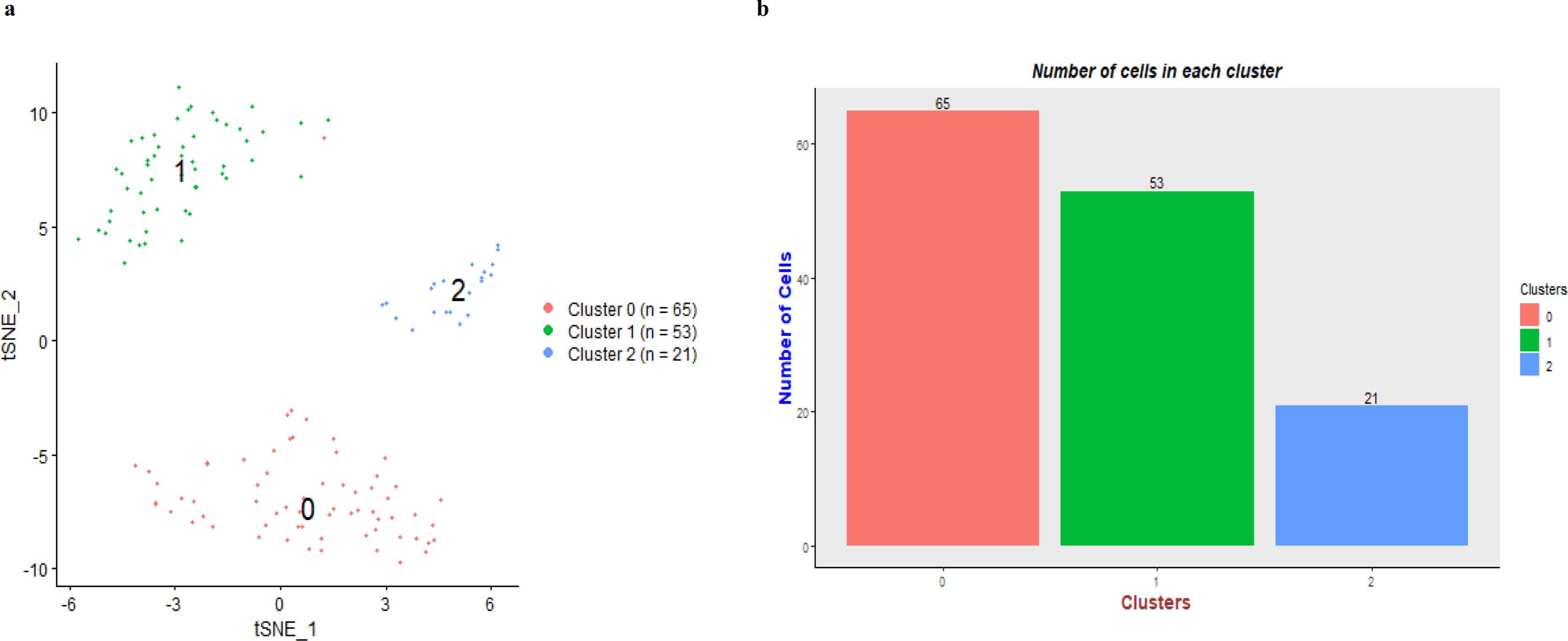
Cell clustering in hepatocellular carcinoma (HCC) dataset. (A) t-SNE plot for cell clustering with 3 clusters, and (B) the bar plot shows the number of cells in individual cluster.

Differential expression analysis

The DE genes were identified in the Differential expression analysis step. After performing filtering (Avg.logFC threshold: 0.585, Min % (min.pct): 0.25, Adjusted P value: .05) on DE gene list, the total number of up-regulated and down-regulated DE genes was 78 and 355, respectively (Figure S20). Cluster 0 detected most of the upregulated genes, and cluster 2 detected the majority of downregulated genes. In addition, violin plots for top-6 upregulated genes (according to logFC) in each cluster are shown in Figure S21. Similarly, the top-6 downregulated genes (according to logFC) for each cluster are shown in Figure S22.

Pseudotime analysis

In our pseudotime trajectory analysis, the tumor cells were stratified according to cell cluster and pseudotime (Figure 3). Cluster 0 cells were assigned with earlier pseudotime, suggesting their potential role as progenitor cells in the HCC development process.

Figure 3.

Pseudotime analysis for the in-house hepatocellular carcinoma (HCC) dataset. Cell trajectory plots based on (A) clusters and (B) pseudotime. Clusters were stratified according to differential pseudotime, with cluster 0 being at putative progenitor-like status.

Liver CSC markers analysis

To further investigate the potential uniqueness of tumor cells of cluster 0 and their putative role as progenitor in cancer development, we examined a panel of liver CSC markers and stemness-related markers. It is found that 9 gene markers (CD24, MYC, CD47, EPCAM, SMO, CTNNB1, KLF4, PROM1, and ABCG2) were highly expressed in cluster 0 (Figure 4). In cluster 0, EPCAM, MYC, and CD47 were the top-3 genes according to the logFC. Taken together, we detected multiple stemness-related or liver CSC markers were significantly and specifically enriched in tumor cells of cluster 0. This evidence is supportive of the suggestive progenitor role for cluster 0 cells in HCC development.

Figure 4.

Liver CSC markers analysis. Violin plots showed the expression of common liver CSC markers according to clusters.

Discussion

In view of the increasing usage of scRNA-seq in various areas of research but there is a lack of analysis tools with graphical interface and comprehensive analytical functionalities, we initiated the current study. First, we developed scAnalyzeR, which is a comprehensive analytical tool for scRNA-seq data with user-friendly graphical interface. It allows scientists with minimal computational knowledge to be able to utilize it. Besides, all the analysis steps in scAnalyzeR are reproducible by taking the advantage of docker platform and versioning system. Importantly, we compared scAnalyzeR with other existing tools with similar developing purposes and demonstrated superior performance as compared to the counterparts. We are aware of other emerging tools, for example, Asc-Seurat²⁷ and will compare the future version of scAnalyzeR against them. Moreover, we also made use of scAnalyzeR to analyze our in-house HCC scRNA-seq dataset and identified interesting findings regarding the identification of progenitor-like tumor cells that expressing multiple stemness-related markers in HCC tumor.

Importantly, scAnalyzeR is aiming to ease the implementation for scRNA-seq study by facilitating the analysis of scRNA-seq data, even for biologists without computation knowledge. Our tool provides full functionality for scRNA-seq data analysis, as well as allows flexibility for users by allowing a wide range of user-defined parameters. A complete user guide is available to illustrate the entire analysis workflow of scAnalyzeR with an example dataset. We hope this tool can be widely adopted by scientists for the convenient analysis of scRNA-seq datasets.

We believe our tool can give a wide range of functionalities to users for scRNA-seq data analysis, although it has some limitations. First, the current version of scAnalyzeR can analyze data of limited species (only 2 species options are available—Human and Mouse). Moreover, it only allows users to upload a single dataset. In the future development, we will accommodate more species and include the functionality of multiple files uploading as it will enable the integration analysis of multiple scRNA-seq datasets. Besides, we have the plan to develop supervised learning method for automatic cell-type annotation, cell–cell interaction analysis, and protein network visualization of the gene sets in pathways. Notably, new dimension reduction and clustering algorithms have emerged,^28–31 and we will consider incorporating them in our future development of scAnalyzeR.

Conclusion

In summary, scAnalyzeR has been evaluated in comparison to other existing scRNA-seq analysis pipelines, in terms of functionalities, execution time, and parameter availability. Moreover, it has demonstrated usability on our in-house liver cancer dataset. We anticipate more functionalities will be adopted to our tool, through the incorporation of other latest packages or algorithms.

Supplemental Material

sj-docx-1-tct-10.1177_15330338221142729 - Supplemental material for scAnalyzeR: A Comprehensive Software Package With Graphical User Interface for Single-Cell RNA Sequencing Analysis and its Application on Liver Cancer

Supplemental material, sj-docx-1-tct-10.1177_15330338221142729 for scAnalyzeR: A Comprehensive Software Package With Graphical User Interface for Single-Cell RNA Sequencing Analysis and its Application on Liver Cancer by GS Chuwdhury, Irene Oi-Lin Ng and Daniel Wai-Hung Ho in Technology in Cancer Research & Treatment

Supplemental Material

sj-docx-2-tct-10.1177_15330338221142729 - Supplemental material for scAnalyzeR: A Comprehensive Software Package With Graphical User Interface for Single-Cell RNA Sequencing Analysis and its Application on Liver Cancer

Supplemental material, sj-docx-2-tct-10.1177_15330338221142729 for scAnalyzeR: A Comprehensive Software Package With Graphical User Interface for Single-Cell RNA Sequencing Analysis and its Application on Liver Cancer by GS Chuwdhury, Irene Oi-Lin Ng and Daniel Wai-Hung Ho in Technology in Cancer Research & Treatment

Footnotes

Abbreviations

Acknowledgements

The authors wish to thank Umme Hafsa for testing the scAnalyzeR and providing valuable feedback during testing. They also thank other group members for suggestions for tool development. The authors also acknowledge other accompanying tools from which scAnalyzeR was developed.

Availability and Requirements

Project name: scAnalyzeR; Project home page: ; Operating system(s): Platform independent; Programming language: R; Other requirements: Docker; License: GNU GPL; Any restrictions to use by non-academics: None.

Authors' Contributions

DWH proposed, designed, and guided the overall study. GSC developed scAnalyzeR, built the docker image, and wrote the usage manual for the software. GSC and DWH tested the software and analyzed the datasets. All provided valuable feedback and suggestions for the functionalities. All wrote and approved the manuscript.

Declaration of Conflicting Interests

The author(s) declared no potential conflicts of interest with respect to the research, authorship, and/or publication of this article.

Funding

The author(s) disclosed receipt of the following financial support for the research, authorship, and/or publication of this article: The study was supported by the National Natural Science Foundation of China (grant number 81872222), Health and Medical Research Fund (07182546), General Research Fund (grant numbers 17100021 & 17117019), Hong Kong Research Grants Council Theme-based Research Scheme (grant numbers T12-704/16-R and T12-716/22-R) and Innovation and Technology Commission grant for State Key Laboratory of Liver Research. I.O.L. Ng is Loke Yew Professor in Pathology.

ORCID iD

Daniel Wai-Hung Ho

Supplemental Material

Supplemental material for this article is available online.

References

Saliba

Westermann

Gorski

, et al. Single-cell RNA-seq: advances and future challenges. Nucleic Acids Res. 2014;42(14):8845‐8860.

Arendt

Musser

Baker

CVH

, et al. The origin and evolution of cell types. Nat Rev Genet. 2016;17(12):744‐757.

Gawad

Koh

Quake

. Single-cell genome sequencing: current state of the science. Nat Rev Genet. 2016;17(3):175‐188.

Butler

Hoffman

Smibert

, et al. Integrating single-cell transcriptomic data across different conditions, technologies, and species. Nat Biotechnol. 2018;36(5):411‐420.

Trapnell

Cacchiarelli

Grimsby

, et al. The dynamics and regulators of cell fate decisions are revealed by pseudotemporal ordering of single cells. Nat Biotechnol. 2014;32(4):381‐386.

Matsumoto

Kiryu

Furusawa

, et al. SCODE: An efficient regulatory network inference algorithm from single-cell RNA-seq during differentiation. Bioinformatics. 2017;33(15):2314‐2321.

Zhang

Luo

, et al. Landscape and dynamics of single immune cells in hepatocellular carcinoma. Cell. 2019;179(4):829‐845. e20.

Chan

Tsui

, et al. Cellular heterogeneity and plasticity in liver cancer. Semin Cancer Biol. 2022;82:134‐149.

Chan

, et al. Molecular pathogenesis of hepatocellular carcinoma. Liver Cancer. 2016;5(4):290‐302.

10.

Zhang

Tsui

, et al.

Single-cell transcriptomics of liver cancer: hype or insights?

Cell Mol Gastroenterol Hepatol. 2022;14(3):513–525.

11.

McCarthy

Campbell

Lun

, et al. Scater: pre-processing, quality control, normalization and visualization of single-cell RNA-seq data in R. Bioinformatics. 2017;33(8):1179‐1186.

12.

Wolf

Angerer

Theis

. SCANPY: large-scale single-cell gene expression data analysis. Genome Biol. 2018;19(1):15.

13.

David

FPA

Litovchenko

Deplancke

, et al. ASAP 2020 update: an open, scalable and interactive web-based portal for (single-cell) omics analyses. Nucleic Acids Res. 2020;48(W1):W403‐w414.

14.

Zhu

Wolfgruber

Tasato

, et al. Granatum: a graphical single-cell RNA-seq analysis pipeline for genomics scientists. Genome Med. 2017;9(1):108.

15.

Guo

Wang

Potter

, et al. SINCERA: a pipeline for single-cell RNA-seq profiling analysis. PLoS Comput Biol. 2015;11(11):e1004575.

16.

Cakir

Prete

Huang

, et al. Comparison of visualization tools for single-cell RNAseq data. NAR Genom Bioinform. 2020;2(3):qaa052.

17.

Merkel

. Docker: Lightweight Linux Containers for Consistent Development and Deployment. 2014. 2014.

18.

Boettiger

. An introduction to docker for reproducible research. ACM SIGOPS Operating Syst Rev. 2015;49(1):71‐79.

19.

Chang

Cheng

Joe

Allaire

, et al. shiny: Web Application Framework for R. R package version 1.4.0. https://CRAN.R-project.org/package=shiny

20.

RStudio Team. RStudio: Integrated Development for R. RStudio, Inc.; 2016. http://www.rstudio.com/

21.

Ihaka

Gentleman

. R: A language for data analysis and graphics. J Comput Graph Stat. 1996;5(3):299‐314.

22.

Xie

Cheng

Tan

. 2019. DT: A Wrapper of the JavaScript Library ‘DataTables’. R package version 0.8. https://CRAN.R-project.org/package=DT

23.

Carson Sievert (2018), plotly for R . https://plotly-r.com

24.

Wickham

Romain

François

Lionel

Henry

, et al. dplyr: A Grammar of Data Manipulation. R package version 0.8.1. https://CRAN.R-project.org/package=dplyr

25.

Wickham

. ggplot2: Elegant Graphics for Data Analysis. Springer-Verlag; 2016.

26.

Tsui

Sze

, et al. Single-cell transcriptomics reveals the landscape of intra-tumoral heterogeneity and stemness-related subpopulations in liver cancer. Cancer Lett. 2019;459:176‐185.

27.

Pereira

Almeida

Conde

, et al. Asc-Seurat: analytical single-cell seurat-based web application. BMC Bioinformatics. 2021;22(1):556.

28.

Liu

. JSRC: a flexible and accurate joint learning algorithm for clustering of single-cell RNA-sequencing data. Brief Bioinform. 2021;22(5):bbaa433.

29.

Zhang

. Network-based integrative analysis of single-cell transcriptomic and epigenomic data for cell types. Brief Bioinform. 2022;23(2):bbab546.

30.

Wang

. Learning deep features and topological structure of cells for clustering of scRNA-sequencing data. Brief Bioinform. 2022;23(3):bbac068.

31.

. Joint learning dimension reduction and clustering of single-cell RNA-sequencing data. Bioinformatics. 2020;36(12):3825‐3832.

Supplementary Material

Please find the following supplemental material available below.

For Open Access articles published under a Creative Commons License, all supplemental material carries the same license as the article it is associated with.

For non-Open Access articles published, all supplemental material carries a non-exclusive license, and permission requests for re-use of supplemental material or any part of supplemental material shall be sent directly to the copyright owner as specified in the copyright notice associated with the article.

0.00 MB

4.36 MB

0.01 MB