
Abstract
Negativity in election campaign matters. To what extent can the content of social media posts provide a reliable indicator of candidates' campaign negativity? We introduce and critically assess an automated classification procedure that we trained to annotate more than 16,000 tweets of candidates competing in the 2018 Senate Midterms. The algorithm is able to identify the presence of political attacks (both in general, and specifically for character and policy attacks) and incivility. Due to the novel nature of the instrument, the article discusses the external and convergent validity of these measures. Results suggest that automated classifications are able to provide reliable measurements of campaign negativity. Triangulations with independent data show that our automatic classification is strongly associated with the experts’ perceptions of the candidates’ campaign. Furthermore, variations in our measures of negativity can be explained by theoretically relevant factors at the candidate and context levels (e.g., incumbency status and candidate gender); theoretically meaningful trends are also found when replicating the analysis using tweets for the 2020 Senate election, coded using the automated classifier developed for 2018. The implications of such results for the automated coding of campaign negativity in social media are discussed.
Introduction
Modern politics is a hard-fought business. The public is increasingly hostile toward those they consider as their rivals (Iyengar et al., 2012; Iyengar & Westwood, 2015), antagonistic and aggressive political figures are on the rise across the globe (Nai & Martinez i Coma, 2019a), and attacks seem at times the very essence of election campaigns (Ansolabehere et al., 1994; Lau & Pomper, 2004). To be sure, negativity in politics matters. Negative information, when compared to equivalent “positive” information, is more likely to be seen, processed, and remembered (e.g., Rozin & Royzman, 2001). Also because of that, some scholars show that negative messages can convey important and useful information to the voters, promote issue knowledge, cue the voters that the election is salient, and thus worth the emotional and cognitive investment, and ultimately stimulate the interest of the public (Finkel & Geer, 1998; Martin, 2004; Geer, 2006). On the other hand, however, strong evidence suggests that negative campaigning can be a detrimental force in modern democracies. Negative and harsh campaigns can reduce turnout and political mobilization, depress civic attitudes such as political efficacy and trust, foster apathy, and generally produce a “gloomier” public mood (Ansolabehere et al., 1994; Thorson et al., 2000; Yoon et al., 2005). On top of this, a case can be made that decreased trust in the political game and increased political cynicism are likely to reinforce the consolidation of antagonistic and disruptive movements, which often “feed” off the public discontent. Whether a positive or detrimental force, few would contest that negativity is a key component of contemporary electoral democracies.
In recent years, the dynamics of electoral campaigning have been reshaped by the emergence of social media (Gainous & Wagner, 2014; Graham et al., 2016; Straus et al., 2013). Online communication, especially via social media, allows political actors to “cut the middlemen”—for instance, journalistic gatekeeping—and communicate directly with their audience, in what is often referred to as “one-step flow of communication” (Bennett & Manheim, 2006). Such facilitated access to the people is one of the reasons why online communication is particularly favored by populists (Engesser et al., 2017). In recent years, several studies have assessed the presence of negativity in social media (e.g., Auter & Fine, 2016; Ceron & d’Adda, 2016; Evans et al., 2014; Evans & Clark, 2016; Gainous & Wagner, 2014; Gross & Johnson, 2016). Broadly speaking, these studies find confirmation that the main trends of strategic campaigning found for traditional techniques—for instance, that challengers tend to attack more than incumbents (Gainous & Wagner, 2014)—are also found when looking at campaigning on social media. Those existing studies tended to rely on manual coding of social media posts. For instance, in their analysis of the drivers of negativity of Facebook during the 2010 Midterms, Auter and Fine (2016) manually coded more than 14,000 posts. Similarly, Ceron and d’Adda (2016) hand-coded more than 15,000 Tweets published by competing candidates prior to the 2013 Italian general election. Recent advances of machine learning approaches have made it increasingly affordable to dive into very large amounts of data, which were inaccessible—or required time-intensive coding efforts—up to recently due to insufficient computational power and the preference for manual coding. In this article, we expand the growing literature on automated classification of textual data within the context of political communication. We introduce a neural network classifier that we trained to automatically annotate the tweets of candidates competing during the 2018 US Senate Midterms elections, in terms of the presence of political attacks. The algorithm was run on approximately 16,000 tweets, posted by 63 candidates for the period between September 1st and November 6th, 2018 (the day of the election). After presenting the results of the classification, the article will test the external and convergent validity of the measure; more specifically, we will check whether the results make sense in terms of factors that can be theoretically expected to drive the presence of negativity in the candidates’ tweets (e.g., the incumbency status of the candidate), and by triangulating the measure with an independent dataset about the content of candidates’ campaigns in the 2018 Midterms, as assessed by expert surveys (Nai & Maier, 2020).
The reason for studying the 2018 midterm elections was two-fold. Firstly, from a conceptual standpoint, the US senate elections provide a unique opportunity to study a series of extremely similar elections with a reduced number of competitors, happening simultaneously within the same broad societal, cultural and, ultimately, political context (Lau & Pomper, 2001, 2004)—while, at the same time, being able to control for the most important differences at the contextual level (e.g., how close the race was). Yet, even if driven by state-level dynamics, Senate Midterms elections all participate to the broader national context and political dynamics. The 2018 Midterms were not an exception in this sense, and the results in each state had fundamental national implications in terms of, for example, the control of the upper house (so central to the recent dynamics of presidential impeachment of Donald J. Trump). In other terms, the Senate Midterms are an ideal research setting, allowing all the benefits of variation—both at the candidate and context levels—while keeping most of the broad cultural and political dynamics, assumed to be shared across all state-level elections at bay, so to speak. Indeed, especially compared with Presidential elections, Senate elections can be seen as “methodologically superior” for the study of campaign dynamics (Lau & Pomper, 2004, p. 6). Secondly, the 2018 Midterm Senate elections provide us with the unique opportunity to test the convergent validity of our data by comparing it with other, independent data about the same elections and the same dynamics (i.e., how negative the candidates in the Midterms went against each other). More specifically, we will triangulate the tone of the candidates’ campaign on Twitter with expert ratings provided by independent scholars (Nai & Maier, 2020).
The rest of this article proceeds as follows. In section 2, we describe the empirical procedure employed to develop the algorithm for the automated coding of the negativity in tweets. Section 3 then presents three tests. First, we test the convergent validity of the algorithm, by comparing it with the measure of negativity from independent data using expert surveys. Second, we test its external validity by checking our measurement against some trends that can be theoretically expected (i.e., the fact that challengers should be expected to be more likely to go negative, or that female candidates tend to use gentler campaigns. Finally, third, we investigate whether applying the coding algorithm to a different set of data—the campaign on Twitter during the 2020 Senate election—yields results that are also theoretically valid. As we will see, our algorithm scores well in both external and convergent validity, suggesting that the automated coding of social media posts is an effective alternative to standard measurement of campaign content. The last section concludes the discussion and glimpses over the directions of future research.
Supporting materials for this article are available at the following Open Science Foundation repository: https://osf.io/up826/. The repository includes (i) the Jupyter Notebook (Python) file with the code that was used to pre-process the raw data, build the classifier, and annotate the whole dataset, (ii) the annotated dataset of all tweets, (iii) the archive with the text of all the collected tweets, and (iv) an excel file with the reliability assessment of the initial sample of tweets coded (see below).
Measuring Negative Campaigning in Tweets
Data and Procedure
During the 2018 Midterms, 33 Class 1 Senate seats were up for grabs (plus additional special elections in Minnesota and Mississippi to fill vacancies, but which we will not analyze here); Democrats were holding 26 of these seats, and Republicans 9. Excluding some scattered small third-party candidates that ran in a handful of elections (e.g., the Libertarian Rusty Hollen in West Virginia), 66 main candidates competed overall to fill these 33 seats, in as many bipartisan races.
The data (tweets) used in this study were collected via vicinitas.io, a website that allows for bulk downloading of tweets retroactively based on Twitter handles (usernames). Prior to it, an online search for Twitter pages of all contemporaneous Senate election candidates was performed to determine which of the candidates used Twitter for their political campaigns and what their Twitter handles were. 1 The handles were then supplied to vicinitas.io to collect the tweets for the period of September 1, 2018–November 6, 2018 (the day of the election), for a total of N = 16,173 tweets. 2 Three candidates did not, to the best of our knowledge, post any tweets in that period (even though they do have a twitter handle): Chele Chiavacci (R, NY, @CheleNYC), Leah Vukmir (R, WI, @LeahVukmir), and Lawrence Zupan (R, VT, @LawrenceZupan). The analyses discussed in this article thus concern the 63 remaining candidates (see Table A1 in Appendix A). The number of tweets per candidate collected varies considerably, from N = 24 for Mitt Romney (R, UT, @MittRomney) to N = 1028 for Rick Scott (R, FL, @SenRickScott), with an average of 256.7 tweets per candidate. Figure 1 plots the number of tweets per day, per party. The figure shows a rather marked increase in the number of published tweets as election day nears, for both parties, similarly to what found in Gross & Johnson (2016) for the 2016 Republican primaries.
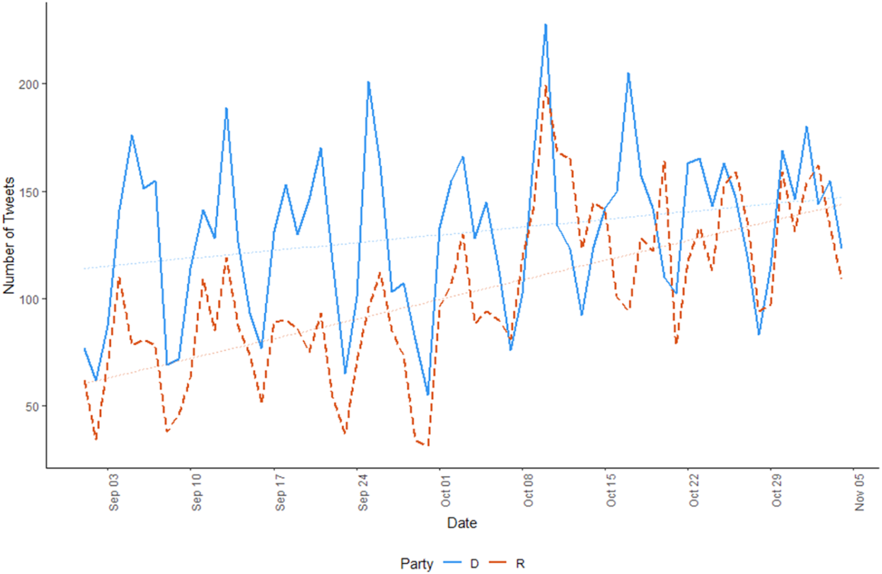
Frequency of tweets per day and party (2018 Senate election).
A codebook was developed to measure the tweets on four dimensions of negativity: negative tone, personal attacks, policy attacks, and incivility. Each of these dimensions was to be coded dichotomously as either present or absent in a given tweet. A random sample of 200 tweets was then coded by four coders independently to assess intercoder reliability. The initial Krippendorff’s alpha reliability scores were .79 for negative tone, .52 for political attacks, 0.50 for personal attacks, and 0.66 for incivility. Given such suboptimal scores, the tweets where disagreements between coders occurred were analyzed by the researchers and the coders were consulted to establish any systematic differences in interpretation of negativity dimensions between the coders. Based on the resulting observations, the codebook was reworked, and its instructions elaborated upon.
Once the coders were briefed on the new instructions, each of them was given a random sample of 100 tweets to annotate. That proved to be insufficient as the negativity dimensions were coded as absent in the overwhelming majority of tweets (M = 89%). Building a successful machine learning classifier presupposes providing a sufficient number of all possible examples during the algorithm training: if there are only a few examples of any given dimension, the model will not be able to accurately generalize the text features that determine the presence or absence of that dimension. To account for such an imbalance, the coders were provided with new random samples of the data and asked to annotate the tweets on one dimension until at least 200 tweets were coded as “present” for the respective dimension. The annotated tweets were then combined producing a dataset of 1186 tweets.
The Algorithm
A multilayer perceptron neural network (MLP; Pedregosa et al., 2011) classifier was trained to automatically annotate the remainder of the tweets. MLP is a type of feedforward neural network where connections between neurons (nodes) do not form loops but are directed onto subsequent layers only, as opposed to recurrent neural networks (RNNs) in which such loops are an integral part. All nodes, with the exception of the input ones, are activated with a non-linear activation function (a function that determines the node’s output given its input), usually a sigmoid or a rectifier, with possible value in the ranges of [−1:1] and [0:1], respectively. The number of hidden layers in the model and the number of neurons in them is chosen freely. All input nodes are connected with a certain weight to all nodes of the first hidden layer, all nodes of the hidden layer are connected to the nodes of the following layer, and so on until the output layer is reached. The initial connection weights are chosen randomly and are adjusted via backpropagation during training (Rosenblatt, 1961).
Using MLP, just like any other neural network, presupposes supplying numeric values, not text, as input values. Consequently, a numeric representation of text (tweets in our case) is required. Such mapping of words (or phrases) to numeric vectors is referred to as word embedding. Multiple techniques have been developed to accomplish the task (c.f. Mikolov et al., 2013; Levy & Goldberg, 2014). For this project, we opted for a pre-trained model from SpaCy owing to its state-of-art performance, compact size, and processing speed. The model 3 includes over 685,000 vectors of 300 dimensions each trained on Common Crawl 4 and OntoNotes 5 5 using convolutional neural networks (Honnibal & Johnson, 2015).
The Procedure
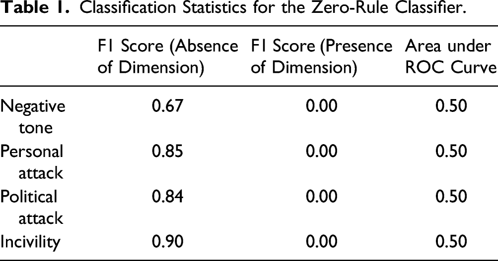
Classification Statistics for the Zero-Rule Classifier.
Next, the data was pre-processed before supplying it to the MLP model. The text of the annotated tweets was “cleaned”: they were stripped of punctuation and single characters, all words were converted to lowercase, and stop-words were removed. Stop words are those words that do not carry any particular information relevant to the meaning of the text, such as “the,” “at,” and “to”; in our case, we use a pre-compiled list of stop words from Spacy.
6
The words also were lemmatized: inflectional endings of words were removed keeping only their “base forms” (lemmas) such that the same words occurring in different grammatical forms across tweets would be transformed into identical ones. Below is an example sentence from one of the tweets (1) in its “raw” format and (2) with the pre-processing steps discussed above conducted: (1) Another example of the corruption our current representation is a part of and the false claims that @SenatorCarper is for the environment. (2) exampl corrupt current represent fals claim senatorcarp environ
Since the stop-word removal and lemmatization are not guaranteed to result in a better classifier performance (sometimes resulting in the opposite effect), four different pre-processed datasets were created with either (1) none, (2 and 3) one, or (4) both of these steps skipped.
As the next step, the words contained in the tweets were vectorized using the pre-trained word-embedding model discussed above and an average vector with 300 dimensions for every tweet was calculated (the number of dimensions is determined by the dimensionality of vectors supplied with the word-embedding model). All out-of-vocabulary words (such as hashtags and mentions) were mapped to zero vectors when computing the average tweet vector. Taking an average of all word embeddings per tweets was done to reduce the processing time needed for the classifier training. 7 As discussed above, vectorizing the input data allowed for (1) representation of words as numeric values required for the next step of model training while (2) preserving the (contextual) meanings of the original words through assignment of similar vector values to words similar in meaning. As the final pre-processing step, the annotated negativity data was reshaped into an array of binary label vectors (e.g., [1,0,0,1] for a single tweet) to allow for a convenient parsing of them into a multi-label MLP model. These transformations resulted in two numeric arrays: one with (1168,300) dimensions for the textual data, and one with (1168,4) dimensions for the negativity dimensions. With both the text and the corresponding label data transformed into the desired formats, we moved onto determining the most fitting hyper-parameters for the data at hand.
To be able to evaluate the model’s performance, 20% of the data (N=234) was set aside as a testing dataset to eventually be used to calculate accuracy statistics of the trained model. Using the remaining 80%, the best parameters were estimated for a multi-label prediction model, a model in which all dimensions of negativity are predicted concurrently. Three-fold cross-validation (i.e., splitting the data into three equal parts and predicting each individual part based on the training of the remaining two) was used to minimize the chance of accidental high performance of the model that is not generalizable to the rest of the data. An alternative approach of training four separate single-label models (one for each negativity dimension) and estimating their hyper-parameters was attempted, too. This was done to see whether greater accuracy can be achieved by fine-tuning independent models rather than having one model predicting all labels simultaneously.
Classification Performance of the Best Model.
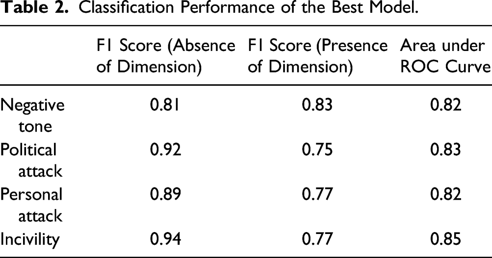
Figure 2 plots the number of negative tweets per day between September and November 2018, separately for Democratic and Republican candidates. The graph shows that Democrats started rather negative but somehow reduced the share of negativity near the end of the campaign. Republicans, on the other hand, rather consistently went more negative as time came close to election day. Frequency of negative tweets per day by party (2018 Senate election).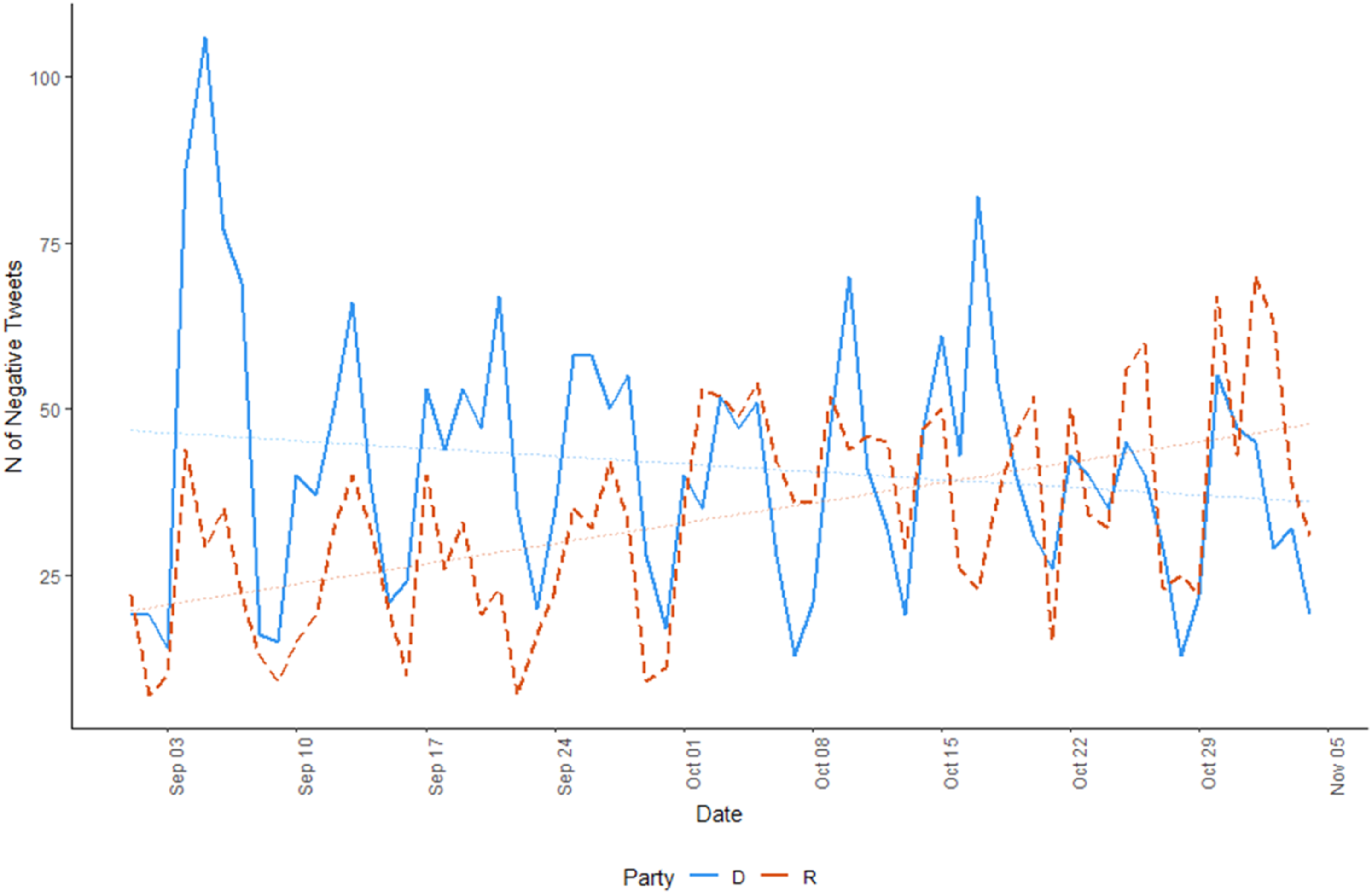
Algorithm Bias
Before moving onto evaluating external and convergent validity of the automatic classification, we assessed the consistency in the algorithm’s predictions and attempted to detect potential systematic errors in its classification. To do that, we leveraged the testing dataset by comparing the true negativity values of the hand-coded tweets to those predicted by the algorithm. Figure 3 presents daily time series of the true and predicted values of all four dimensions of negativity (the time series were smoothed using a 7-day moving average). The figure suggests that the algorithm is consistent in its predictions of the negativity dimensions and does not significantly deviate from the true values at any time. Seven-day moving average of true and predicted values of the four negativity dimensions by day (2018 Senate election). Note. The figure also includes standard deviations of the difference between the true and predicted values for each of the negativity dimensions (top right corner).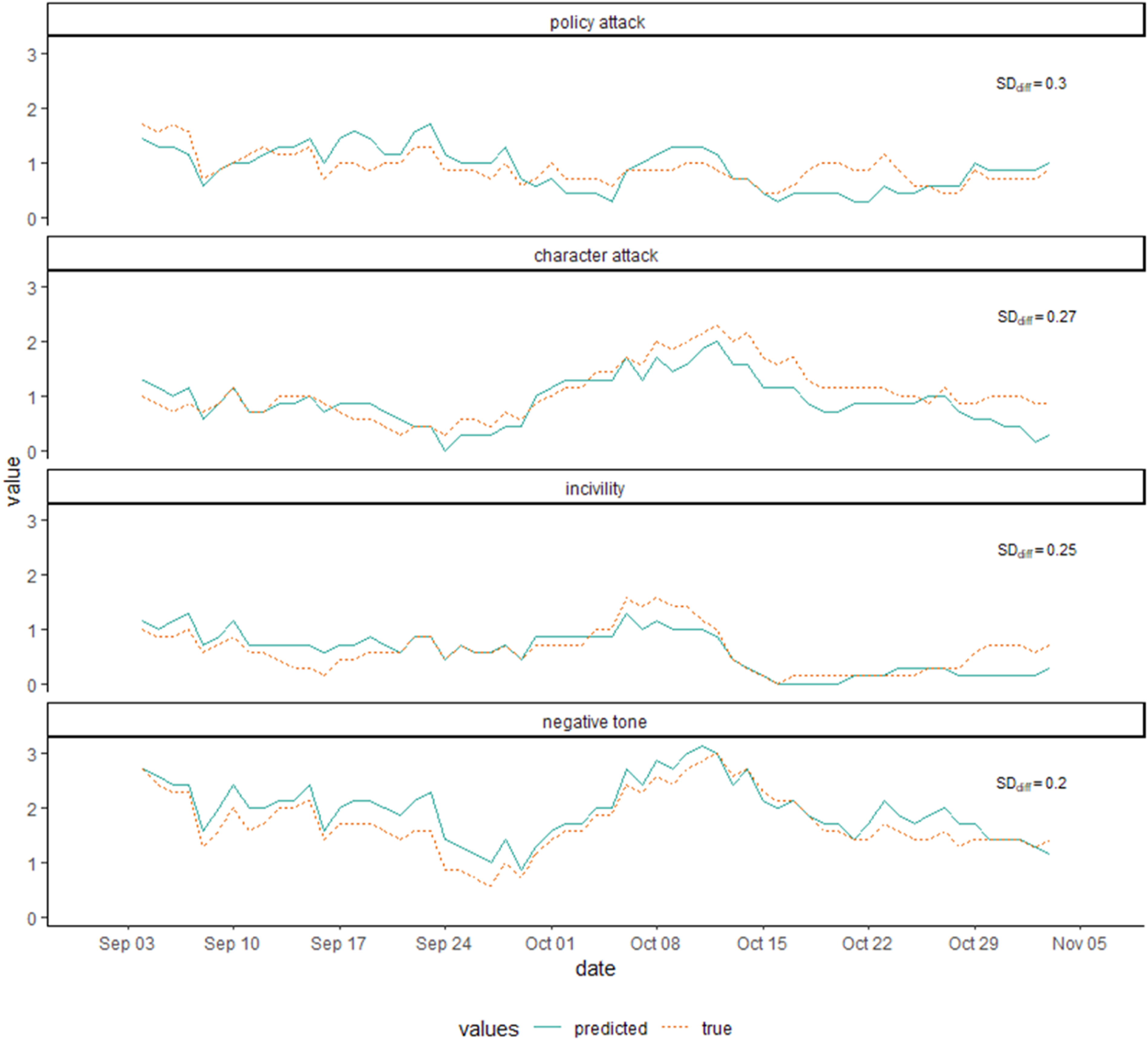
For a more formal analysis, we ran a series of chi-square tests comparing the frequencies of the presence and absence of negativity between the manually annotated and predicted tweets. Separate chi-square tests were run for tweets posted by different groups of candidates to see whether the algorithm performs equally well under all circumstances. The difference between the true and predicted values were assessed for tweets subset by candidates’ party, gender, incumbency status, state-level race closeness, and state level of Trump support in the 2016 presidential elections. In total, 48 chi-square tests were performed, with none indicating a significant difference between the true and predicted values. Additionally, we performed topic modeling using density-based clustering (Campello et al., 2013) on the entire dataset (extracting 15 topics such as discussions of economic policy or encouragements to cast a vote) to check whether the algorithm’s performance is consistent over different topics. Chi-square tests comparing the true and predicted negativity values were run for each topic with all tests producing statistically insignificant results. Finally, we also performed correlation analyses to determine whether there is a relationship between the candidates’ frequency of posting and the candidates’ average negativity scores (on all four dimensions). These tests also produced no statistically significant results. Together these analyses suggest that the algorithm’s performance is consistent and unbiased.
Testing the Algorithm
We present below three sets of analyses that we implemented to test for the convergent and external validity of our developed algorithm. The first test (convergent validity) checks whether the measurement of campaign negativity from our algorithm yields results that are in line with other, independent measurements of the same phenomena, in our case expert judgments about the campaign content of candidates having competed in the 2018 Senate elections (Nai & Maier, 2020). The second test (external validity) checks whether our measurement is theoretically meaningful, that is, is able to show trends that reflect string theoretical assumption—in our case, regarding the drivers of campaign negativity. Finally, the third test (replication) tests whether applying the coding algorithm to a different set of data—the campaign on Twitter during the 2020 Senate election—yields results that are also theoretically valid. As we will discuss below, all three sets of tests yield positive results for our algorithm.
Convergent Validity: Negativity in Twitter and Expert Ratings
Convergence
Valid new constructs should ideally be in line with similar existing constructs. We test here convergent validity by comparing our Twitter measures of negativity with completely independent data gathered within the framework of an expert survey (Nai & Maier, 2020). In the direct aftermath of the 2018 Midterms, we distributed a standardized survey to a sample of scholars with expertise in elections, politics, or political communication working for a US higher education institution. Among other things, experts were asked to evaluate the content of campaigns of the two competing candidates for the Senate in that state. We were not able to gather any expert opinions for North Dakota and West Virginia, and only one expert provided ratings for candidates in Hawaii, Nevada, and Wyoming, which we excluded from our analyses for robustness reasons; only candidates for whom at least two scholars provided independent ratings are included in our analyses. Analyses are run for the remaining 49 candidates (see Table A1 in Appendix A).
The number of experts that answered our survey varies between 2 (e.g., for Delaware) and 30 (California), with an average of 8.04 experts per candidate. Table A1 in Appendix A lists all candidates and presents how many experts rated their campaign. On average, experts in the sample lean unsurprisingly to the left (M = 3.22/1-10, SD = 1.43); 66% of them identify as a Democrat, 21% as Independent, and only 4% as a Republican (4% prefer not to say). 27% of them are female. Experts rated themselves as quite familiar with election campaigns in their state (M = 7.81/0-10, SD = 2.05) and estimated that the survey was easy to answer (M = 7.52/0-10, SD = 2.39).
Experts were asked to rate to what extent candidates used “negative campaigning” against their opponent during the election, that is, to what extent they relied on campaigning messages “criticising their opponents’ programs, ideas, accomplishments, qualifications, and so forth.” For each candidate, they provided a rating between −10 “Very negative” and +10 “Very positive,” which we simplified into a 0-10 negativity scale where 10 means “Very negative.” Experts also had to evaluate whether candidates attacked mostly on policy issues or on the personal characteristics and character of their opponents, using a scale from 1 “Exclusively policy attacks” to 5 “Exclusively character attacks.” For the sake of comparison, we transformed this variable into a 0-10 scale, where 10 means “Exclusively character attacks.” Finally, experts were asked to what extent the candidates used “fear appeals,” on a 0-10 scale where 10 means “very high use.”
Unsurprisingly, the three measures are strongly correlated, for example, for fear and tone, r(52) = .75, p < .001, and would load into an additive scale, α = 0.87. An exploratory factor analysis (PCA) extracted a single underlying factor explaining 81% of the variance (Eigenvalue = 2.42), with factor loadings between 0.56 and 0.60. This underlying factor varies between −2.91 and +2.81 and can be seen as a broad measure of campaign negativity, as assessed by experts. Amy Klobuchar (D, MN) and David Baria (D, MS) are the two candidates with the lowest scores of campaign negativity according to our experts, whereas Corey Stewart (R, VA) and Matt Rosendale (R, MT) score the highest. Table A1 in the Appendix includes the scores, for each candidate, on both the Twitter and experts’ measures of negativity.
To what extent are the two independent measures of campaign negativity—the automated coding of tweets and the broad assessment by election experts—associated? Before answering this question, it is important to stress that the two measures do not necessarily reflect the same phenomenon: the automated measure is specific to the content of campaigns is social media (on Twitter, more precisely), whereas experts were asked to assess the campaign of candidates in general, regardless of the medium. It is known that the use of negativity differs across different communication channels (Walter & Vliegenthart, 2010). Some candidates, for instance, might go very negative in TV ads, and only use Twitter to promote events. In this sense, we should not expect that the two measures are a perfect reflection of each other. Nonetheless, we could expect that both are a proxy of the underlying campaigning style of each candidate, and we thus expect them to be associated somehow.
Table 3 regresses the three measures of campaign negativity via the automated coding of tweets on the expert’s assessment of candidate negativity (underlying index), controlling for the usual suspects that drive negativity discussed in the previous section. Perception of campaign negativity is a function of both the content of each ad (or, in this case, tweet) and the total volume of ads (tweets) people are exposed to (e.g., Stevens, 2009); for instance, a candidate with very negative tweets but having posted only a handful of them would probably be perceived as much less negative than a candidate with fewer negative tweets on average but much more activity on social media. We take this into account by using in our analyses the volume of negativity in tweets, that is, the average content of tweets for each candidate (in terms of tone, policy attacks, and character attacks) multiplied by the total number of tweets posted by that candidate. Models in Table 3 are hierarchical linear models, where candidates are nested within states.
Negativity on Twitter by Expert Assessments (2018 Senate Election).
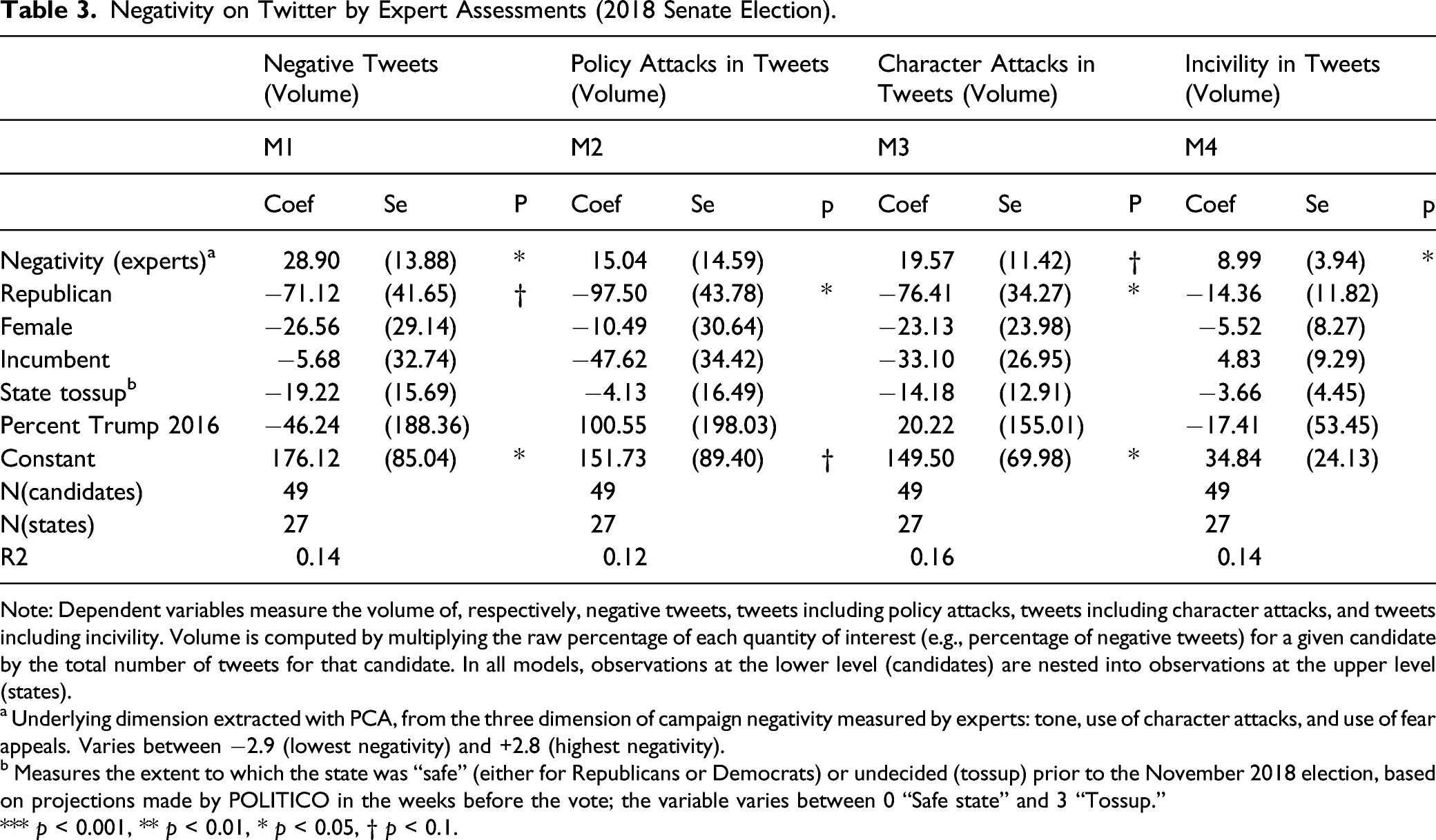
Note: Dependent variables measure the volume of, respectively, negative tweets, tweets including policy attacks, tweets including character attacks, and tweets including incivility. Volume is computed by multiplying the raw percentage of each quantity of interest (e.g., percentage of negative tweets) for a given candidate by the total number of tweets for that candidate. In all models, observations at the lower level (candidates) are nested into observations at the upper level (states).
a Underlying dimension extracted with PCA, from the three dimension of campaign negativity measured by experts: tone, use of character attacks, and use of fear appeals. Varies between −2.9 (lowest negativity) and +2.8 (highest negativity).
b Measures the extent to which the state was “safe” (either for Republicans or Democrats) or undecided (tossup) prior to the November 2018 election, based on projections made by POLITICO in the weeks before the vote; the variable varies between 0 “Safe state” and 3 “Tossup.”
*** p < 0.001, ** p < 0.01, * p < 0.05, † p < 0.1.
Results in Table 3 suggest that the two measures are associated, once controlling for the candidate profile, the closeness of the race, and the percent of votes for Trump in the state in the 2016 Presidential election. Campaigns that are evaluated by the experts as very negative (underlying dimension) have a volume of negativity on Twitter that is twice as high as campaigns that are evaluated as very low in negativity (M1). A similar trend exists for the volume of incivility (M4) and character attacks on Twitter (M3), albeit less strongly. We do not find a significant association between experts’ negativity measure and the volume of policy attacks on Twitter (M2), which might be due to the fact that the expert measure mostly picked up the harsher components of campaign negativity (harsher personal attacks and fear appeals). All in all, however, the expert general perceptions of candidates’ negativity and the volume of tweets coded as negative (and containing character attacks), as coded by our algorithm, go hand in hand quite strongly, and in the expected direction—even controlling for powerful drivers of campaign negativity, to which we turn in section 3.2.
Divergences
To be sure, for some candidates the level of negativity in their campaigns diverges quite considerably from what estimated by experts. In order to uncover any substantial patterns in this sense, we have computed for each candidate the distance between the volume of negativity on Twitter (coming from our algorithm) and the estimated volume of negativity predicted by our inferential model (Table 3, M1). We have computed such residual (M = 0.0, SD = 83.9) in such a way that positive values indicate that the model underestimated the volume of negativity when compared to the measurement produced by the algorithm, and negative values indicate the opposite (experts overestimated, or the algorithm is more conservative) (see Table D1 (Appendix D) for all divergence scores). By far the most extreme case when it comes to underestimation by the model is represented is Corey Stewart (R, VA). Even accounting for the fact that experts assessed Mr. Steward as having run a very negative campaign, the volume of negative tweets he employed was off the charts, much higher than what the model estimated. This is unlikely to be outlandish. Stewart is known for his “Trumpian” style, affiliations to ultranationalists, and frequent harsh comments against more moderate Republicans (Nwanevu, 2018). As such, it is actually likely that the algorithm correctly picked up the very extreme campaign run by Mr. Stewart, not only in absolute terms but also in comparison to all other candidates—something that experts were of course unable to do. On the other end of the spectrum we find Geoff Diehl (R, MA), Robert Flanders (R, RI), and Jon Tester (D, MT), for whom the algorithm measured less negativity than it was predicted by the model—perhaps indicating that these candidates campaigned more negatively on other channels. Perhaps as a confirmation, Mr. Tester is among the candidates having used the higher share of negative TV ads (64%), as attested by the Wesleyan Media Project (WMP; Fowler et al., 2020). 8
The presence of these outliers is both a cautionary tale and a reassuring finding. On the one hand, it indicates that even if the convergent validity check was successful, extreme cases for which the algorithm is less successful cannot be excluded. On the other hand, the fact that these extreme cases can be explained logically is reassuring and allows for a better understanding of what the algorithm picks up (and not).
External Validity: What Drives Negativity?
Beyond convergent validity, any relevant measure must be able to tell something about the broad phenomenon it captures. Thus, an additional important test for the validity of a measure is to assess to what extent it is useful to predict known dynamics, or it is predicted by known drivers. In our specific case, we test to what extent some known drivers of negativity are associated with the presence or absence of attacks in the tweets. If we expect our algorithm to effectively capture tweet negativity, then we ought to expect that cases in which negativity should be expected to be greater should be more likely to be represented by tweets classified as negative, broadly speaking. It is important to note here that we are not interested in discussing the drivers of campaign negativity on social media. Rather, our substantive point in this section (and the following) is that being able to find theoretically relevant patterns when using our algorithm to code the content of campaigns in social media is likely to indicate, in our opinion, that the algorithm is measuring something that is substantively valid, above and beyond its technical components.
Why, and under which circumstances are candidates competing in elections more likely to go negative on their rivals? Research on the drivers of negative campaigning, even if comparatively less developed than research in its effects, provides some cues. First, consistent evidence in the US and internationally suggests that incumbent candidates are less likely to go negative (e.g., Lau & Pomper, 2004; Gainous & Wagner, 2014; Nai, 2020). The rationale here is two-fold. On the one hand, because they previously held an office, incumbents have experience and records to showcase, and have thus greater incentives to go positive; challengers often do not have such a possibility, and are thus more naturally driven to attack the incumbents (Nai, 2020), whose record while in the office is in any case already closely scrutinized by the public at large; because voters tend to rely on retrospective evaluations to make up their mind (Healy & Malhotra, 2013), challengers naturally try to expose bad deeds and inconsistencies in their opponent’s record, program, and character. The fact that challengers receive comparatively a weaker media coverage than incumbents (Hopmann et al., 2011) should also act as incentive to go more negative, in the light of evidence showing that negativity is much more likely to attract media attention that positivity (e.g., Geer, 2012). On the other hand, incumbents have much to lose—much more so than challengers—and should thus be more wary of the potentially negative effects of harsh attacks; the public usually tend to dislike harsh campaigns (Fridkin & Kenney, 2011; Johnson-Cartee & Copeland, 1989), and candidates that go excessively negative face the risk of backlash effects where their net favorability in the eyes of the voters drops—instead of the target’s (Shapiro & Rieger, 1992; Roese & Sande, 1993). Many scholars have shown that the prospect of electoral failure is a catalyst to adopt a more negative rhetoric (Harrington & Hess, 1996; Walter et al., 2014; Nai & Sciarini, 2018). Negative campaigning aims at reducing support for (and favorability of) the opponents; a candidate that starts with a comparative disadvantage (e.g., lagging behind in the polls) “has not succeeded in attracting undecided voters and, therefore, has to scare off the opponent’s voters to stand a better chance” (Elmelund-Praestekaer, 2010, p. 141). Given that incumbents naturally start with a strong comparative advantage over challengers (Cox & Katz, 1996), these latter should face extra incentives to go negative. In their analysis of negative campaigning on Twitter during the 2016 Republican primaries, Gross & Johnson (2016) also find that candidates tended to “punch upwards” (excluding Donald Trump, an exception on many aspects).
Second, some evidence exists that candidates or the right-hand of the political spectrum are more likely to go negative. In the USA, Lau and Pomper (2001) and Gainous and Wagner (2014) show that Republican candidates are more likely to go negative than Democrats, which might perhaps be because GOP strategists have been shown to be more open to the idea of strategic attacks (Theilmann & Wilhite, 1998). On the other hand, some marginal evidence exists that voters identifying with the Democrats are, under some conditions, less sympathetic toward negativity than Republicans or independents (Ansolabehere & Iyengar, 1995; Mattes & Redlawsk, 2015). These trends seem to exist outside of the USA as well; in Switzerland, the most negative party by far during referenda campaigns is the far-right Schweizerische Volkspartei (SVP—Swiss People’s Party; Nai & Sciarini, 2018), and an analysis of 172 candidates competing in elections worldwide shows that, indeed, the likelihood of going negative is higher for candidates on the right (Nai, 2020).
Third, we might expect female candidates to be less likely to go negative (but see Maier, 2015; Evans et al., 2014; Evans & Clark, 2016). Even today, reasons still exist to imagine women have a strategic disadvantage, compared to men, when adopting a more negative or harsher rhetoric. Social stereotypes generate shared expectations that female candidates should be passive, kind, and sympathetic (Huddy & Terkildsen, 1993; Fridkin et al., 2009; Krupnikov & Bauer, 2014), and harsh rhetoric clearly contrasts with these stereotypes, generating potentially stronger backlash effects (Kahn, 1996; Trent & Friedenberg, 2008).
The conditions of the race should also shape the strategic considerations leading to the decision to go negative (or not). Some authors suggest that more competitive or “close” races should lead to more negative campaigns because the stakes tend to be higher (Kahn & Kenney, 1999; Lau & Pomper, 2004; Elmelund-Praestekaer, 2008); yet, the opposite is also found (e.g., Francia & Herrnson, 2007). Given what is discussed above for incumbents, we believe that close situations should decrease the use of attacks in a case such as the US Senate elections. In elections with uncertain results, risk aversion should play a particularly important role; on the other hand, if elections run in “safe” states, the risks of nefarious backlashes should be lower for both challengers and incumbents: the former have probably little to lose, and for the latter any backlash effects are unlikely to put a decisive dent in their chances to secure a victory. We might thus expect negativity to be especially high during elections fought in “safe” states. Finally, evidence exists linking the timing of the campaign with the use of more negative messages, so that little remaining time before the vote increases negativity (Ridout & Holland, 2010; Damore, 2002; Nai & Martinez i Coma, 2019b). According to most existing studies, negative campaigning is more likely to be effective for candidates that are seen as credible on the issues at stake—which is mostly achieved with positive campaigning. In other terms, “by waiting to go negative until after they have established themselves in the mind of voters, candidates may be perceived as more credible, which may increase the veracity of their attacks” (Damore, 2002, p. 673). On the other hand, and following the main rationale discussed above for incumbency and competitiveness of the race, late attacks might be ever riskier, and the time to correct potential backlash effects is limited. In this sense, a rationale could also be developed why negativity should decrease when election day looms—especially when the election is close.
Drivers of Negativity on Twitter (2018 Senate Election).
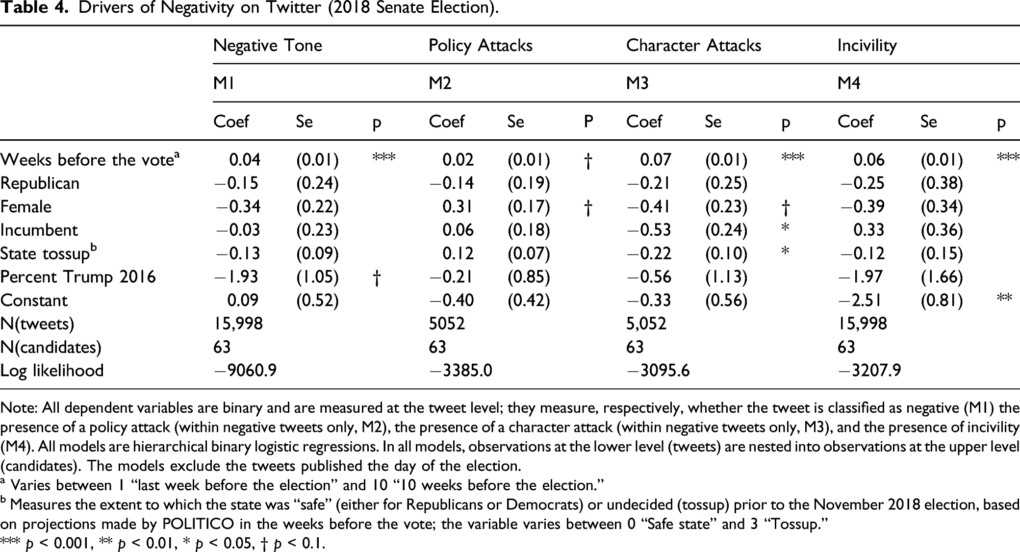
Note: All dependent variables are binary and are measured at the tweet level; they measure, respectively, whether the tweet is classified as negative (M1) the presence of a policy attack (within negative tweets only, M2), the presence of a character attack (within negative tweets only, M3), and the presence of incivility (M4). All models are hierarchical binary logistic regressions. In all models, observations at the lower level (tweets) are nested into observations at the upper level (candidates). The models exclude the tweets published the day of the election.
a Varies between 1 “last week before the election” and 10 “10 weeks before the election.”
b Measures the extent to which the state was “safe” (either for Republicans or Democrats) or undecided (tossup) prior to the November 2018 election, based on projections made by POLITICO in the weeks before the vote; the variable varies between 0 “Safe state” and 3 “Tossup.”
*** p < 0.001, ** p < 0.01, * p < 0.05, † p < 0.1.
Table 4 shows several results that are in line with our expectations. Incumbents are less likely to use character attacks (M3), in line with the idea that incumbents have much to lose if they are excessively harsh. Inversely, female candidates are more likely to use policy attacks (M2) and less likely to run character attacks (M3) than their male counterparts, confirming the idea that female candidates have incentives to stay away from harsher attacks that are potentially at odds with social gender stereotypes. No significant results appear for the candidate’s partisanship, even if Republican candidates seem marginally to have been less negative overall. Given that the Democrats were generally more active on Twitter than the Republicans during the time period analyzed, the proportion of negative tweets to all tweets posted by a given party was also considered. While there was no significant difference in the average levels of negative tone between the parties, Republican candidates had a significantly larger proportion of tweets containing character attacks (p < 0.001, M = 0.04) and incivility (p = 0.003, M = 0.02) while the Democrats had a larger proportion of tweets containing policy attacks (p = 0.002, M = 0.03). However, considering that (1) perception of campaign negativity is a function of both the content of each ad (or, in this case, tweet) and the total volume of ads (tweets) people are exposed to (e.g., Stevens, 2009), and (2) comparison of the overall volume of negative tweets produces no significant results, these minor differences in negative dimensions between the parties are likely inconsequential. Turning to the campaign conditions, tweets during elections fought in competitive states—in our case, states whose result was expected to be a likely tossup 9 —are less include harsher character attacks (M3). The effect is relatively substantial; marginal effects show that the estimate share of character attacks tweets goes from about 22% in “tossup” states to about 36% in “safe” states. Finally, tweets published late in the race are less likely to be negative, uncivil, and if negative they are less likely to use harsh character attacks. This effect contradicts usual trends in the literature, suggesting that the end of the race tends to increase in negativity and harshness (e.g., Ridout & Holland, 2010; Nai & Martinez i Coma, 2019b), but could make sense in light of the effects shown for incumbency and closeness of the race: when the stakes are higher (in this case, little remaining time), risk averse behaviors kick in and negativity goes down.
A Replication Check: The 2020 Election
An even more severe test for the external validity of our automated measurement is to assess whether it is also able to predict theoretically meaningful dynamics in another election. To do this, we have used the algorithm developed for the 2018 election, discussed in this article so far, to classify the content of Tweets published by candidates having competed in the 2020 Senate election. In the November 2020 election, 33 Class 2 Senate seats were contested (plus additional special elections in Arizona and Georgia to fill vacancies, which we will not analyze here); 12 were previously held by Democrats and 21 by Republicans. Out of all candidates competing in the (mostly) two-party races for these seats, we were able to collect the Twitter posts for 63 of them (Table A2, Appendix A). 10 We collected via vicinitas.io all tweets published by these candidates for the period between August 29, 2020 and November 3, 2020 (the day of the election), matching the length of data collection used for 2018. A total of total of N = 24,762 tweets were collected, an increase of 53% compared to 2018. The number of tweets per candidate collected varies considerably, from N = 3 for Ben Sasse (R, NE, @SenSasse) to N = 2055 for John Cornyn (R, TX, @JohnCornyn), with an average of 393.0 tweets per candidate. These tweets were classified using the algorithm developed for the 2018 election (i.e., the same MLP classifier fitted on the manually annotated data from the 2018 election was used).
Drivers of Negativity on Twitter (2020 Senate Election).
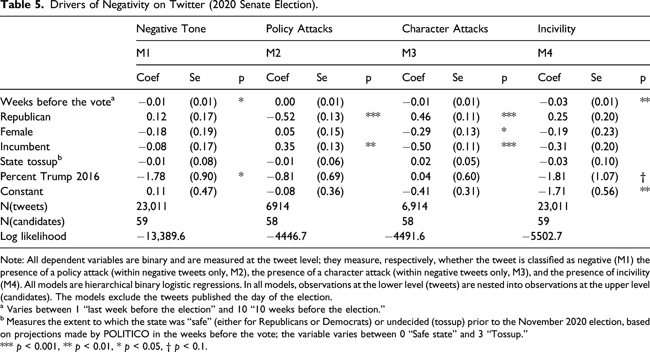
Note: All dependent variables are binary and are measured at the tweet level; they measure, respectively, whether the tweet is classified as negative (M1) the presence of a policy attack (within negative tweets only, M2), the presence of a character attack (within negative tweets only, M3), and the presence of incivility (M4). All models are hierarchical binary logistic regressions. In all models, observations at the lower level (tweets) are nested into observations at the upper level (candidates). The models exclude the tweets published the day of the election.
a Varies between 1 “last week before the election” and 10 “10 weeks before the election.”
b Measures the extent to which the state was “safe” (either for Republicans or Democrats) or undecided (tossup) prior to the November 2020 election, based on projections made by POLITICO in the weeks before the vote; the variable varies between 0 “Safe state” and 3 “Tossup.”
*** p < 0.001, ** p < 0.01, * p < 0.05, † p < 0.1.
As for 2018, and in line with the literature, results for 2020 indicate that the harshest attacks (character attacks) are significantly less likely for incumbents and for female candidates (M3). Furthermore, incumbents were more likely to prefer policy attacks when going negative (M2; this trend was also present in 2018, but the coefficient was not significant).
Interestingly, Table 5 presents two instances of results that match the theoretical expectations discussed above but were not present in 2018. First, general negativity and incivility increase as the election day nears, as shown in the literature (Ridout & Holland, 2010; Damore, 2002; Nai & Martinez i Coma, 2019b). Second, Republican candidates were significantly more likely to use character attacks and less likely to use policy attacks (the effect of being a Republican on the presence of attacks in general and the use of uncivil messages is positive, but not significant), also in line with American and comparative research showing a greater propensity for right-wing candidates to go negative (Lau & Pomper, 2001; Gainous & Wagner, 2014; Nai, 2020). Additional models (Appendix C) show furthermore that Democrats and Republicans use different attacks depending on the political leaning of the context in which they campaign. As substantiated in Figure 4 with marginal effects, Democrats increasingly use character attacks in Republican states (high percentage of Trump votes in 2016) and policy attacks in Democrat strongholds (low percentage of Trump votes in 2016). Inversely, Republicans use more character attacks in Democratic states, and policy attacks in Republican states. Taken together, these results indicate that in more unfavorable contexts both Democrats and Republicans tend to prefer a more confrontational approach via harsher attacks, but rely on constructive, policy attacks in their strongholds—reflecting the general idea that conflict spawns conflict (Maier & Nai, 2021). Probability of attack by candidate leaning and percent votes for Trump in 2016; marginal effects (2020 Senate election). Note. Marginal effects, with 95% confidence intervals. Dependent variable is the probability that the tweet was coded as negative (top left-hand panel), as containing a policy attack (within negative tweets only; top right-hand panel), as containing a character attack (within negative tweets only; bottom left-hand panel), and as uncivil (bottom right-hand panel). Full results are in Table C1 (Appendix C).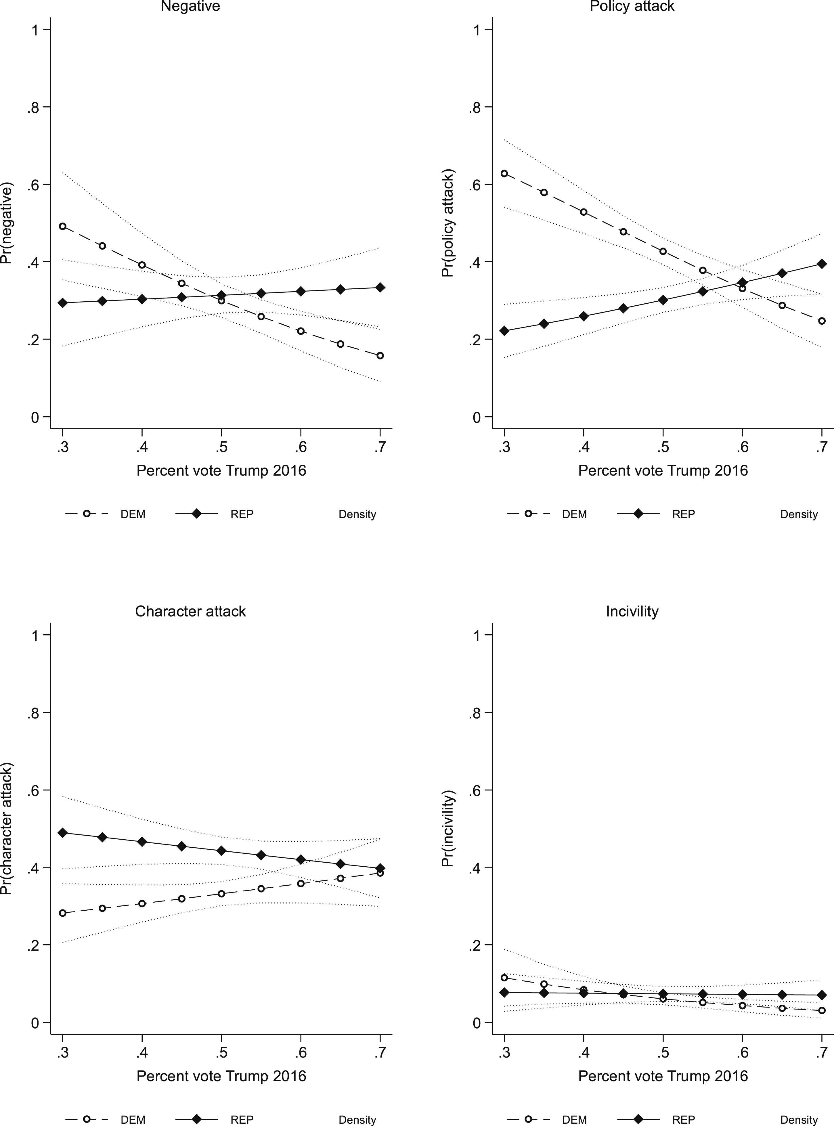
All in all, trends for 2020 are theoretically meaningful, suggesting that our automated measurement comes with a strong potential for replication in different contexts, on top of performing well in convergent and external validity.
Applications and Limitations
All in all, the results discussed in the previous sections seem to indicate that automated classifications are able to provide reliable measurements of campaign negativity. Triangulations with independent data show that our automatic classification is strongly associated with the experts’ perceptions of the candidates’ campaign. Furthermore, variations in our measures of negativity can be explained by theoretically relevant factors at the candidate and context levels (e.g., incumbency status and candidate gender); theoretically meaningful trends are also found when replicating the analysis on tweets published by candidates during the 2020 Senate election, coded using the automated classifier developed for 2018.
These results face some caveats. First, if the dataset at the tweet level was relatively consequential, it represented a restricted number of candidates overall. Studying the campaign behavior of candidates in the US senate elections offers multiple advantages (Lau & Pomper, 2004), but due to the mechanism of electoral competition in the US only about 60 candidates are actually competing for open seats in any given Midterm election. To be sure, the data at hand was large enough to test for the driving effect of characteristics at the candidate and context levels. Yet, the relatively small N prevented us for more nuanced analyses, especially in terms of composition effects—for instance, it could be argued that the gender plays a different role for Democrats and Republicans, but testing for such moderating effects would stretch the data too thinly. Second, the dynamics discussed in this article reflect a very narrow electoral setting, which only rarely finds a match outside of the US. At odds with the imperative of expanding our current knowledge of negative campaigning outside of the abundantly studied US case (e.g., Nai and Walter, 2015), our article plays the card of simplicity versus innovation when it comes to case selection. To be sure, there are several excellent reasons for selecting the US Senate Midterms for our study; yet, further research is direly needed to confirm the exportability of US results in different settings. Third, and relatedly, the jury is out regarding the exportability of our algorithm to textual data in other languages (but see, e.g., Huang et al., 2013).
Finally, some critical questions about the process behind algorithmic classification of negativity still remain to be answered. Although our tests suggest that the new automatic classification method exhibits satisfactory performance and is generalizable to other contexts, a lot remains unknown about what features the algorithm considers relevant and how exactly it decides on its classification of negativity. Yet, transparency in the algorithmic classification process is important: not only to be able to definitively assess the features’ theoretical relevance and justifiability, but also to better detect possible systematic errors in the algorithm’s predictions. Recent developments in explainable artificial intelligence (XAI) have sparked the creation of a number of frameworks aimed at opening the “black box” of machine learning algorithms. These frameworks rely on various mathematical models that attempt to approximate the black box model’s predictions (globally or locally) while still allowing for interpretability of the results. Some of the widely used frameworks include LIME (Ribeiro et al., 2016), which uses local linear approximations to mimic the black box model’s behavior, and SHAP (Lundberg & Lee, 2017) which borrows from game theory and utilizes Shapley values for model approximation. Regardless of the employed method, all of these frameworks aim to discern which features, and to what extent, contribute to the classification result. Employing them in future research on automated classification of negativity can shed some light on the algorithmic decision-making process and elucidate how robust and context-independent it is. Doing so can further strengthen the case for usability of automated measures of negativity and help discern in which scenarios such measures are most effective and in which less so.
With these limitations in mind, it is important to explicitly state what we believe the best usages for our algorithm are. First, from a practical standpoint, our algorithm can be used to assess the level of negativity in upcoming elections that reflect the structural and institutional patters of elections investigated here—that is, single-seat elections with a small number of competing candidates elected via plurality voting. This can be either done post-hoc once the election is over, or be scaled up as an interactive tool for real-time campaign assessment. But, given the materials on which the algorithm was developed, we strongly advocate against the use of the algorithm for the classification of elections under, for example, a plurality formula, where the absence of a zero-sum game makes it much more complicated to assess automatically who the target of attacks and incivility might be (and who might benefit from it). Second, from a methodological standpoint, our algorithm can however serve as a starting point to develop expanded classifications of campaign negativity that are less contingent on the institutional circumstances we faced here. Finally, and within the parameters discussed above, our algorithm can be used to provide independent external validity checks for all scholars engaged in content analysis of election campaigns in traditional communication channels, such as TV ads. Being largely automated, quite cost-effective, and scalable for large datasets, the algorithm ticks all the boxes for validity checks.
Discussion and Conclusion
The study of campaign messages has only recently turned toward the candidates’ communication in social media (Gainous & Wagner, 2014; Graham et al., 2016; Straus et al., 2013). Several studies assessed the presence of negativity in social media (e.g., Auter & Fine, 2016; Ceron & d’Adda, 2016; Evans et al., 2014; Evans & Clark, 2016; Gainous & Wagner, 2014; Gross & Johnson, 2016), and broadly confirmed that the main trends of strategic campaigning found for traditional techniques—for instance, that challengers tend to attack more than incumbents (Gainous & Wagner, 2014)—are also found when looking at campaigning on social media.
Within this framework, our article introduces a neural network classifier that we trained to automatically annotate the tweets of candidates competing during the 2018 US Senate Midterms elections. The algorithm, trained on approx. 1000 tweets, was run on over 16,000 tweets, posted by 63 candidates for the period between September 1st and November 6th, 2018 (the day of the election) to classify the presence of political attacks (both in general and separately for policy and character attacks) and the use of incivility. Safe for the description of the algorithm construction, the bulk of the article was dedicated to a series of tests, showing the performance of our algorithm in terms of external and convergent validity of the measure. The first series of tests assessed the convergent validity of our measure. To do so, we compared it with independent data gathered within the framework of an expert survey (Nai & Maier, 2020). Controlling for several determinants at the candidate and state levels, our results show that campaigns that are evaluated by the experts as very negative (underlying dimension) have a volume of negativity on Twitter that is twice as high as campaigns that are evaluated as very low in negativity; a similar trend exists for the volume of incivility and character attacks on Twitter, albeit less strongly. All in all, this suggests high convergent validity of our automated measure of negativity on Twitter.
The second series of tests checked whether our automated measure “makes sense” in terms of factors that can be theoretically expected to drive the presence of negativity in the candidates’ tweets. Our results show that consistently with evidence in the US and internationally (e.g., Lau & Pomper, 2004; Nai, 2020), incumbents are significantly less likely to go negative on their rivals. Also, in line with the theory (e.g., Kahn, 1996; Trent & Friedenberg, 2008), female candidates are less likely than their male counterparts to run harsher character attacks and more likely to attack on policy. Our results also show that tweets in competitive states are less likely to be negative and uncivil, and that tweets published late in the race are less likely to be negative, uncivil. This last effect is at odds with results found elsewhere (e.g., Ridout & Holland, 2010; Nai & Martinez i Coma, 2019b), but makes sense in light of the effects shown for incumbency and closeness of the race: when the stakes are higher (little remaining time), risk averse behaviors are probably triggered, reducing the chances that candidates go negative. The third series of tests took the external validity check a step further, and assessed whether the classifier developed for the 2018 election is able to provide a theoretically meaningful measurement of the tone of campaigns on Twitter for a different election altogether—the 2020 Senate election. Results show that as for 2018 (and in line with the literature), results for 2020 indicate that character attacks are significantly less likely for incumbents and for female candidates, and that incumbents were more likely to prefer policy attacks when going negative. In 2020, we also find several results that perfectly match the theoretical expectations, but were not present in 2018: negativity increases as the election day draws near, and Republican candidates were significantly more likely to use character attacks and less likely to use policy attacks. An additional series of models showed furthermore that both Democrats and Republicans tend to use harsher attacks in states controlled by the other party, in pine with the general idea that more conflictive contexts provide incentives for harsher campaigns (Maier & Nai, 2021). The fact that results are at times different from the trends showed for the 2018 election suggest that contextual determinants are quite likely to play an important role as well. The 2020 election was a rather different political event than the 2018 one, for many reasons—it included a presidential contest, whereas the 2018 only featured elections for the House and the Senate, and of course it took place in a unique political context marred by extreme polarization and the unfolding drama of the COVID-19 pandemic. These contextual drivers are likely to alter the dynamics at play and affect the incentives for candidates to go negative. Yet, the fact that for both the 2018 and 2020 elections the trends shown are broadly in line with the theoretical expectations reinforces our main claim that our automated classifier is able to yield an externally valid measurement of campaign negativity.
Our article contributes by expanding the state of the art in computational research for political communication. From a practical point of view, it demonstrates that automatic classification is a viable and efficient method for content analysis of campaign negativity. Researchers can rely on this method in the future to investigate dynamics of negative campaigning across parties and elections, the relationship between negativity and electoral outcomes, and drivers of campaign negativity, among other things. Furthermore, from a theoretical perspective, by enriching the tools at our disposal to measure negativity, our article indirectly contributes to a broader understanding of negative campaigning dynamics. As discussed above, our measure confirmed some established trends in the literature when it comes to the drivers of negative campaigning in elections. The mammoth task at hand now is to deepen our understanding of its consequences. Does negativity work as intended, by increasing the electoral prospect of the attackers while at the same time reducing support for the target? Does negativity mobilize or demobilize? And, on the long term, is negativity nefarious for our current standards of liberal democracy? It is not our goal here to develop on these fundamental, normative questions. We conclude by simply suggesting that fine-grained measurements of candidate negativity in social media have potentially an important role to play for these questions. Figure 5 plots the frequency of attacks per day, and depending on whether the candidate ultimately won or lost the race for the seat. Frequency of policy attacks per day and election outcome (2018 Senate election).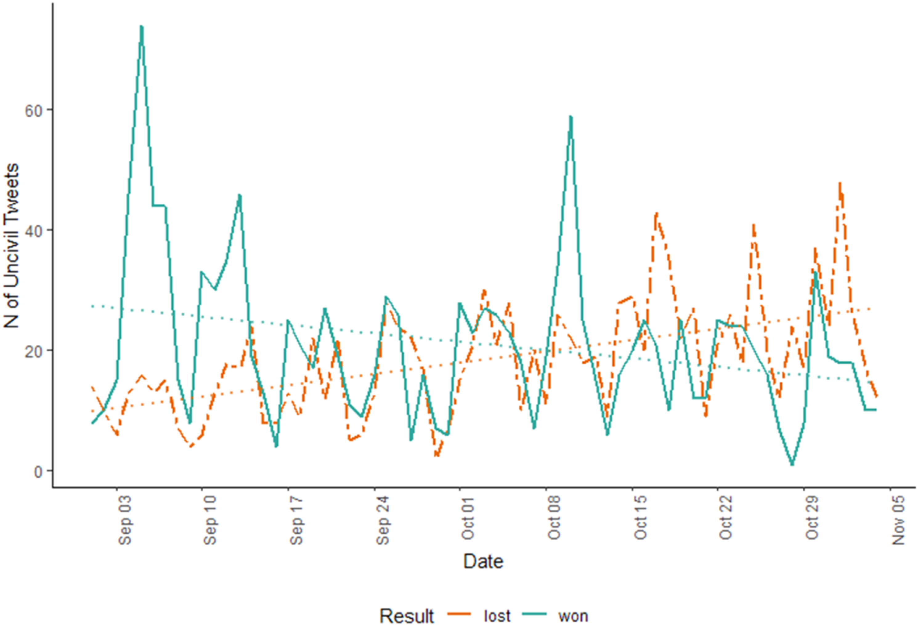
The figure seems to indicate a trend where an increase of negativity over time is associated with electoral defeat, in line with the idea that negativity is a risky business. To be sure, this simple association is not enough to conclude that (an increase in) negativity has detrimental effects on electoral results. The relationship between the use of attack politics and electoral success could very well be reversed so that candidates lagging behind in the polls and facing an electoral defeat could face enhanced incentives to attack (e.g., Skaperdas & Grofman, 1995; Harrington & Hess, 1996; Nai & Martinez i Coma, 2019b). The dynamics of attack politics and electoral support are complex, and likely to be marred by two-sided causality—negativity can drive more (un)favorable electoral standings in polls, which in turn set up (dis)incentives to go negative subsequently, and do forth (e.g., Blackwell, 2013). Such fine-grained analysis that also requires intermediate assessments of electoral standings (e.g., poll data) is beyond the scope of this article. But the data at hand is particularly appropriate to disentangle such nuanced dynamics, and further research in this sense is under way.
Footnotes
Acknowledgements
We are very grateful to the journal editor and anonymous reviewers for their careful reading and constructive suggestions, and to Sebastian Stier and Jürgen Maier for precious inputs and feedback. All remaining mistakes are of course our own. Lieke Bos, Camilla Frericks, and Nilou Yekta were instrumental for data collection and coding – thank you! Finally, a sincere thanks to all experts that have donated their time to participate in our expert survey in the aftermath of the 2018 Midterms – and to those who are currently participating in the parallel expert survey covering elections worldwide. We will pay it forward.
Declaration of Conflicting Interests
The author(s) declared no potential conflicts of interest with respect to the research, authorship, and/or publication of this article.
Funding
The author(s) received no financial support for the research, authorship, and/or publication of this article.