Sage Journals: Discover world-class research

Abstract

Electrospinning is one of the leading techniques for fiber development. Still, one of the biggest challenges of the technique is to control the nanofiber morphology without many trial-and-error tests. In this study, it is demonstrated that via design of experiments (DoE), response surface methodology (RSM) and machine learning regressions (MLR) it is possible to predict the beads-on-string size, size distribution and bead density in electrospun poly(vinylidene fluoride) (PVDF) mats with a small number of tests. PVDF concentration, dimethylacetamide/acetone ratio, tip-to-collector voltage and distance were the parameters considered for the design. The results show good agreement between the experimental and modeled data. It was found that concentration and solvent ratio play the main roles in minimizing bead size and number, distance tends to reduce them, and voltage does not play a significant role. As an evaluation of the potential of the method, bead-free fibers were obtained through the predicted parameter values. Comparison of the performance of the two methods is presented for the first time in electrospinning research. Response surface methodology resulted much faster, but MLR achieved a lower error and better generalization abilities. This approach and the availability of the MLR script used in this work may help other groups implement it in their research and find information hidden in the data while improving model prediction performance.

Keywords

electrospinning poly(vinylidene fluoride)response surface methodology machine learning regressions prediction and optimization bead formation

Introduction

Electrospinning technique is more than a century old and has been intensely studied for the last two decades, but it remains a growing area of material and technology research for its unending possibilities. Furthermore, in the last few years, its use has grown in the industry as an innovative filter with very desirable attributes.¹ One of its outstanding applications is the development of poly(vinylidene fluoride) (PVDF) electrospun filters for high-efficiency face masks regarding the covid-19 outbreak.²

Electrospinning consists in the formation of micro-nanofiber nonwovens by electrically charging and ejecting a polymer solution. The solution is pumped through a spinneret under a high-voltage electric field, and solution jets are shot to the opposite electrode (collector). On the way to the collector, bending instability takes place and the jets are extremely stretched, thinned and bent. In this stage, the solvents evaporate, and thin polymer fibers are deposited over the collector. The interaction between the physical parameters in this stage is not yet fully predictable by theory. Common applications of electrospinning technology are air filtration,^3,4 water remediation,^5–8 drug delivery,^9,10 and wound dressing,¹¹ among others.¹²

Electrospun fibers often have beads which are considered defects or by-products. Bead formation in electrospun fibers is caused by the instabilities of the polymer solution jet, where surface tension, viscoelastic forces and electric forces (determined by charge density, conductivity of the solution, and tip-to-collector voltage and distance) compete for the contraction or stretching of the solution jet.¹³ Surface tension leads to droplet formation and capillary breakup, but for polymer solutions, instead of breaking, filaments between the droplets are stabilized and a bead-on-string structure is formed. The reason for this is the elongation and entanglement of the macromolecules of the dissolved polymer, which form a network that persist as the fiber solidifies.¹⁴ Overall, it has become clear that bead formation is related to the complex interactions between the solution properties and electrospinning process parameters,¹⁵ and for this reason, it is still an experimental matter to observe carefully.

Although the formation of such beads on fibers is widely spread over electrospinning research and production,¹⁶ is not commonly addressed, and remains an issue of interest as it is undesirable in many cases, and desirable in others. In air filtration research, the presence of beads on electrospun fibers has been correlated with lower pressure drop while maintaining high filtration efficiency.¹⁷ The presence of beads broadens the distances among the fibers, which lowers the air pressure drop of the membranes.^18,19 Evenly distributed beads in the fibers create a more even pore distribution, which inhibits the aggregation of dust particles during air filtration.²⁰ On the other hand, bead structure of the nanofibers contributes to high specific surface area and surface functional groups, which improves filtration efficiency.²¹ Overall, the filtration quality factor of beads-on-fiber electrospun membranes was found to be higher than that of bead-free fibers.^22–24 Presence of beads on electrospun fibers has also been correlated with improvements in mechanical properties of the mats,^23,25 enhanced hydrophobicity,²⁶ and Na-ion storage advantages.²⁷ In most applications, however, bead-free fibers are more desirable.²⁸

In several works, for the same polymer and solvents choice, dissimilar concentrations have been reported as optimal to obtain bead-free fibers.^29–31 This is reasonable as some of the variables of the process which are not commonly considered may change from one work to the other. Molecular weight, inner diameter of tip, temperature and relative humidity and overall electrospinning chamber geometry are not always reported in electrospinning studies, although they have been found to affect the morphology of the obtained fibers.^32–35 The variability in these factors results in inconstancy of the optimum values of typical electrospinning parameters (i.e. solution concentration and solvent ratio, voltage, tip-collector distance, and flow rate). For these reasons, whenever electrospinning research starts, it is common to use the parameters of previous works, and then change them according to one’s own experimental results. However, the usual protocol for optimizing electrospinning parameters is to change one variable at a time, which is a rather expensive and time-consuming methodology.³⁶

In past research, a great number of tests were needed to find the empirical relations between a set of electrospinning parameters and PVDF nanofibers surface structure.^37,38 No single work has studied the morphology of the electrospun PVDF nanofibers by varying every electrospinning parameter, and therefore, if one or more of the fixed parameters are changed in a new study, the literature values are not reproduced. This fact, added to the variability of electrospinning equipment (open surface, multi-needle, different geometries, etc. ³⁹), and the time optimization required in industrial processes, leads to the necessity of finding a way to achieve the desired electrospun nonwoven morphology without an excessive number of trial-and-error tests.

Response surface methodology (RSM) and machine learning regressions (MLR) are valuable predictive tools to reduce the number of trials necessary to find the optimal set of parameters, especially when a high number of variables are at play. Response surface methodology explores the relationships between factors affecting a process and response variables obtained from the output of that process. It uses a sequence of designed experiments to obtain a desired (optimal) response. Machine learning regressions are programs that “learn” and model the relations between features (input variables) and targets (response variables) from datasets. The empirical models that result from these algorithms predict the response variables in non-explored data points. The algorithms adjust themselves to perform better given feedback on their past performance in predictions about the same dataset. These regressors have been used in several applications with great performance,⁴⁰ and they have outperformed RSM in some studies.⁴¹

Electrospinning is a good candidate for these tools because of the large number of experimental parameters and the difficulty to theoretically predict their effect on the response variables or targets. Also, to reduce the number of tests necessary to optimize the output. Response surface methodology was proposed several times to address this issue, obtaining good results for fiber-size optimization,^42–44 pore size and fiber quality,⁴⁵ bead number,^46,47 bead size,⁴⁸ and other applications.⁴⁹ Some works have made use of machine learning algorithms such as artificial neural networks to minimize electrospinning fiber diameter⁵⁰ and some have compared its performance to that of RSM.^51,52 Few works have been found which used MLR predicting power to optimize the electrospinning process.^53–55 Ieracitano et al. have recently used machine learning algorithms to identify beads on electrospun fibers,⁵⁶ but to the best of our knowledge, MLR have not been used to study the bead formation process. Furthermore, no works have been found which compare MLR and RSM performances for the same experimental design of the electrospinning process.

The objective of this study is to investigate the ability of two different models to predict the size and number of beads-on-fibers for the important case of PVDF electrospun nonwovens: the traditional RSM and a promising approach by MLR. PVDF electrospun micro and nanofibers have been prepared with different sets of parameters, encountering dissimilar beads. The influence of the polymer concentration, solvent ratio, voltage and tip-to-collector distance over the bead size and overall bead density, was modeled through RSM and MLR. The parameters which minimize the targets in each model were investigated through experimental testing, and both models' performances were compared. This work presents a method to achieve the desired mat morphology without an excessive number of tests, addressing the not yet fully understood relation between electrospinning parameters and bead formation, which may be useful regarding the massive use of electrospinning technique. Also, it compares the challenges and performances of a traditional method (RSM) with a machine learning regressor that has never been used in electrospinning optimization.

Experimental section

Materials

Polyvinylidene fluoride (PVDF) powder (Mw = 534.000 g mol⁻¹) and N,N-dimethylacetamide (DMAC, ≥99.0%) were purchased from Sigma-Aldrich. Acetone (≥99.5%) was purchased from Biopack. All reagents were used without further purification. Table 1 shows the viscosity, electric conductivity and surface tension of the solvents.

Table 1.

Physical properties of the used solvents.

Solvent	Viscosity (cP)	Conductivity (10⁻⁴ S m⁻¹)	Surface tension (10⁻³ N m⁻¹)
DMAC	1.02 ± 0.01 (20°C)	1860 ± 30 (26.6°C)	36.7 ± 0.1 (20°C)
Acetona	0.32 ± 0.01 (20°C)	0.38 ± 0.03 (25°C)	23.3 ± 0.1 (20°C)

Preparation of PVDF solution

Poly(vinylidene fluoride) was dissolved in a two-solvent mix of DMAC and acetone by a magnetic stirrer for 4 h at room temperature in a sealed reservoir. The polymer concentration was varied between 15.8 and 20 wt% and DMAC/acetone w/w ratio between 1.2 and 2.9.

Electrospinning

A scheme of the electrospinning device used in this work is shown in Figure 1. The plain metal collector and the single nozzle were horizontally faced inside a rectangular acrylic chamber. The PVDF solution was added to a 10 mL syringe with a needle tip (21G, 0.5 mm inner-tip diameter). A high DC voltage power supply was utilized to generate the electric field between the electrodes, ranging between 8 and 16 kV, and the tip-to-collector distance was varied from 10 to 35 cm. The solution feed rates were controlled by a syringe pump, ranging from 0.1 to 1.0 mL h⁻¹ for preliminary tests (see Supporting Information), and then fixed at 0.2 mL h⁻¹. The samples were obtained by electrospinning over glass coverslips (18 × 18 mm²) attached to the collector for time intervals between 2 and 15 min. All experiments were carried out at room temperature (24.0 ± 1.5)°C and ambient relative humidity (50 ± 3)%.

Figure 1.

Schematic of the electrospinning setup.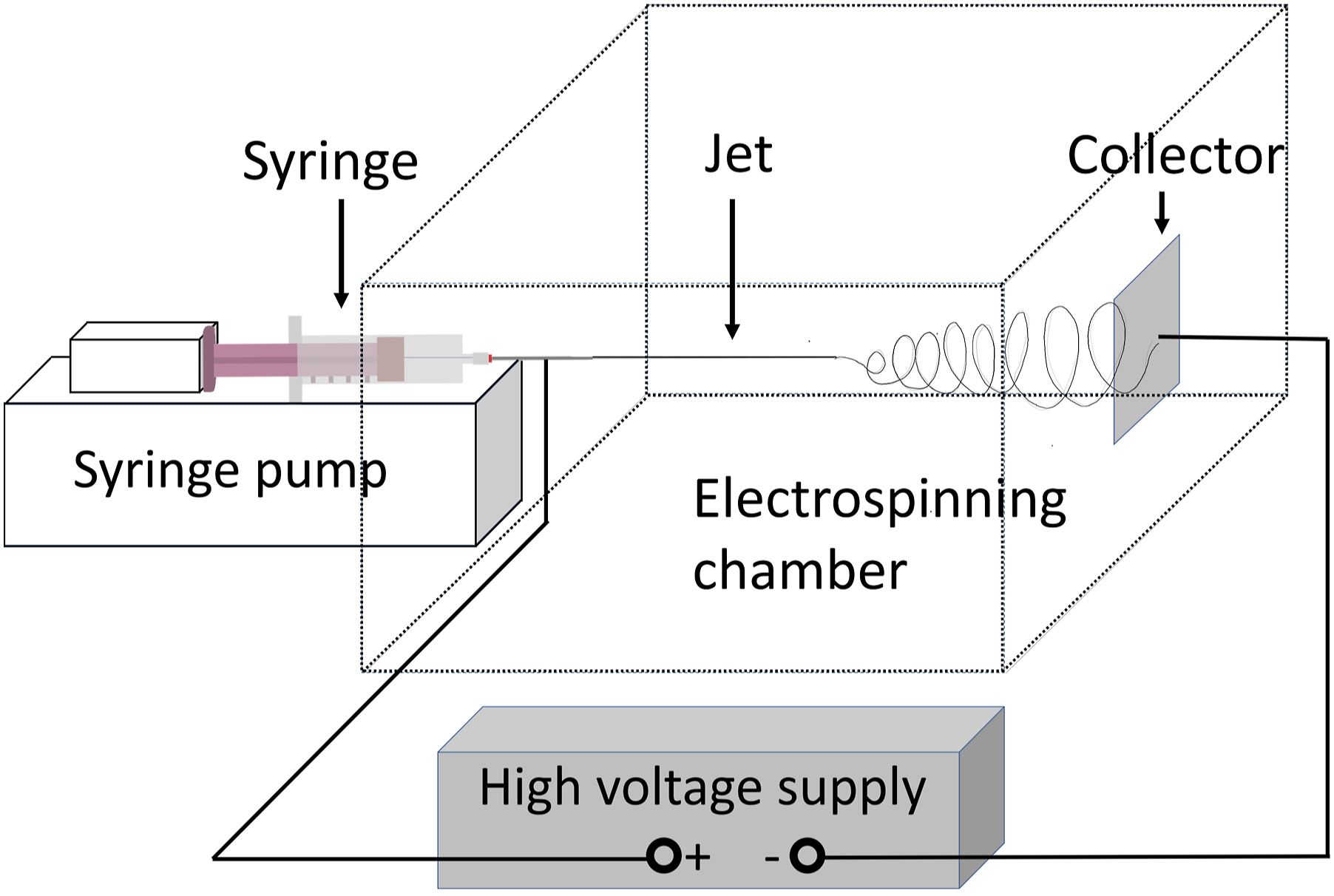

Image analysis

Four images of each electrospun sample were obtained through an Olympus BX60MF5 Optical Microscope (100x) and then processed through ImageJ software. The size of each individual bead was obtained. Given the range of bead sizes found in this work (5–25 μm), optical microscopy was preferred. It allows capturing, in a single picture, larger areas than scanning electron microscopy (SEM), which helps in image processing. It is also faster and cheaper.

Field Emission Scanning Electron Microscopy (FE-SEM Carl Zeiss NTS - SUPRA 40) was used to reveal the micro-nano scale morphologies of optimized electrospun fibers. Samples were previously sputtered with platinum.

Experimental design

Design of experiments is a valuable tool to reduce the number of experimental tests needed to find an approximate relation between some input variables (features), and the response variables (targets). Consequently, it allows predicting response variables of unexplored data points. In this study, a custom I-optimal split-plot design was implemented via Design-Expert software to investigate the relation between the input variables: PVDF concentration (c), ratio between solvents (r), voltage (V) and distance (d) between tip and collector, and the response variables: beads mean equivalent diameter (BMED), standard deviation (Sdev) and bead density (BD). The bead equivalent diameter (BED) was calculated as in equation (1) where AB is the area of the bead in the nonwoven-plane as seen from the microscope image (measured with ImageJ software), and the BMED is the mean of the BED found in the microscope images of one sample. The Sdev is the standard deviation of the BED in each sample, which gives an estimation of the regularity of the bead size throughout the sample.

B E D = 2 \sqrt{\frac{A B}{π}}

(1)

The last target is the bead density, calculated as the number of beads per mm² of electrospun mat. Given that each mat sample has a slightly different thickness and fiber density, a normalization calculation was included.

The split-plot was created to take into account the difference between the hard-to-change factors and the ones that are easy to change. Both PVDF concentration and DMAC/acetone ratio are hard-to-change parameters because they depend on the solution, and it takes hours to make a new solution to restart the electrospinning process. On the other hand, the voltage and tip-to-collector distance may be easily modified during the electrospinning process within seconds. Therefore, it is of interest to provide the algorithm with the least amount of c and r combinations of values necessary. I-optimality was chosen as it has been shown to outperform other criteria regarding improved predicting.⁵⁷

Nine tests were taken mapping the parameters space of the two hard-to-change factors, as shown in Figure 2. The black squares in the graph represent points in the desing space that achieved PVDF bead-free fibers according to literature, using DMAC/acetone solvent system. Therefore, the range of values of each feature was considered by analogy with bibliography and by preliminary tests. The full data (varying voltage and distance) consisted of 126 points. Table 2 shows the value ranges chosen in this work for the four parameters. For voltages under 8 kV the electric field was not enough to eject the solution. For voltages above 16 kV, the jets broke leading to short segments of polymer fiber.

Figure 2.

Design space of the hard-to-change factors: PVDF concentration and DMAC/acetone ratio (blue circles). Black squares: parameters that lead to bead-free PVDF fibers according to literature (1:⁵⁸; 2:⁵⁹; 3:⁶⁰; 4:⁶¹; 5:⁶²; 6:³⁰).

Table 2.

Limit values of the features in the design space.

Feature	Min	Max
PVDF concentration (wt%)	15.8	20
Ratio between solvents (w/w)	1.2	2.9
Voltage (kV)	8	16
Tip-collector distance (cm)	10	35

Response surface methodology

Quadratic, cubic, and quartic basis functions were tested to establish approximation responses in this study, selecting only the most influential coefficients through backward elimination (p-value < 0.1) and respecting hierarchy. The choice of polynomial degree was done through studying the different responses and analysis of variance (ANOVA). Verification of the response was done experimentally as it is customary for this kind of model.⁶³

Machine learning regressors

Data were split into training and testing sets (75-25%). This is a common practice, as it allows testing accuracy of the model in unseen data. Four supervised machine learning algorithms were utilized: Ridge regressor (RR), support vector regressor (SVR), random forest (RF), and voting regressor (VR).

Ridge regression addresses some of the problems of ordinary least squares by imposing a penalty on the size of the coefficients, preventing overfitting.⁶⁴ The implemented algorithm minimized the loss function E_RR shown in equation (2), where y_i is the response variable for the i_th sample and ${\hat{y}}_{i}$ the predicted value. The weight w_j is squared, multiplied by an L2 penalty term (λ) and added to the residual sum of squares. λ is the parameter that controls the amount of shrinkage, i.e. the reduction in the effects of sampling variation: the larger the value of λ, the coefficients become more robust to collinearity; if λ is set to 0 then the entire equation becomes like a normal Linear Regression curve.

E_{R R} = \sum_{i = 1}^{N} {(y_{i} - {\hat{y}}_{i})}^{2} + λ \sum_{j = 1}^{D} w_{j}^{2}

(2)

In this study, RR is fitted in conjunction with a polynomial regression, considering not only linear terms of the variables but also higher orders.

Support vector machines create decision boundary lines from hyperplanes to separate samples in categories and use the kernel trick to map the data into a higher-dimensional feature space.⁶⁵ SVR is an extension to regression problems by considering close samples as similar. The algorithm implemented in this study minimizes equation (3), where C is a penalty term that trades off residual error against simplicity of the response surface. f(x) is the solution regression function (equation (4)), where α_i is the i_th Lagrange multiplier and k(x,x‘) is the kernel function. In this study, radial basis function (RBF) (i.e. $e^{- γ {‖ x - x^{'} ‖}^{2}}$ ) was used as kernel. RBF introduces the hyper-parameter γ, that defines how much influence a single training sample has. The larger γ is, the closer other samples must be to be affected.

m i n C \sum_{i = 1}^{n} {| y_{i} - f (x) |}^{2} + \frac{1}{2} {‖ w ‖}^{2}

(3)

f (x) = \sum_{i}^{n} α_{i} k (x, x')

(4)

Random forest is a regression model that combines many decision trees, trained through bagging. Tree-based methods split the feature space into even chunks (branches) and fit a simple model to each one, while bagging is an ensemble algorithm that improves the accuracy of machine learning individual estimators. RF predicts by taking the average of the output from various trees.⁶⁶ In this study, two RF hyper-parameters were considered: the number of estimators (n), and the maximum number of branches (depth). Increasing n improves the precision of the outcome. Increasing the maximum depth allows better fitting but also may lead to overfitting.

The script was written in python, using Scikit Learn package, which has the in-built function of cross-validation (CV). This allows splitting the data into different groups (folds) and training a regressor holding out one group of data sequentially, which acts as a validation set. The performance of the algorithm is evaluated by some chosen metric in each of the unseen folds of each split, and then the average metric value is considered. This way, the generalization ability of the model is evaluated and optimized during the training. A scheme of the CV can be seen in Figure 3.

Figure 3.

Schematic diagram of the framework proposed in this study.

The three algorithms were fitted to the training data (after scaling if necessary) via GridSearchCV (5-fold cross-validation) to find the hyper-parameters that minimized the root mean squared error (RMSE) for the validation set. The RMSE is a measure of the deviation between the predicted and the actual values, as shown in equation (5), where N is the number of data points. Table 3 shows the hyperparameter values tested in each algorithm.

R M S E = \sqrt{\frac{\sum_{i = 1}^{N} {(y_{i} - {\hat{y}}_{i})}^{2}}{N}}

(5)

Table 3.

Hyperparameter values evaluated through cross-validation.

	Polynomial degree	Lambda (λ)
Polynomial features with ridge regression	1, 2, 3, 4, 5, 6, 7	10⁻³, 10⁻², 10⁻¹, 1, 10, 10², 10³, 10⁴
	C	Alpha (α)
Support vector machine regressor with SBR kernel	1, 10, 10², 10³, 10⁴, 10⁵, 10⁶	10⁻⁴, 10⁻³, 10⁻², 10⁻¹, 1, 10
	n estimators	Max depth
Random forest	10, 50, 100, 300, 500, 700	2, 3, 4, 5, 7, 10, 15

Finally, a weighted voting regressor (VR) was implemented to create an ensemble meta-model that combined the three previous optimized algorithms. This type of regressor can be useful for a set of similarly well-performing but conceptually different models, to balance out their individual weaknesses and avoid systematic errors. The VR was evaluated in the test set, and the predictions of the model were studied by looking experimentally into the values of the optimized features.

Figure 3 shows the whole scheme of this work, from the experimental design and tests, the image analysis and modeling methods, to the final experimental validation.

Results and discussion

The BMED, Sdev and BD histograms are shown in Figure 4(a). The three targets follow normal or slightly positively skewed distributions with respective mean values of (15.7 ± 2.9) μm, (6.0 ± 2.5) μm and (66 ± 43) mm⁻² and Pearson’s first skewness coefficient of 0.38, 0.33 and 0.85 respectively. Figure 4(b) shows the correlation matrix for the whole dataset (correlation between features was omitted). The Pearson coefficient shows that large BMED values are highly correlated with high Sdev values, therefore, minimizing bead size will likely reduce their size dispersion as well, resulting in a more regular morphology. Increasing the distance between tip and collector seems to generally reduce the values of the three targets, tending to the formation of small and regular beads or bead-free mats. Polymer concentration and solvent. Ratio also have a noticeable incidence in the targets. Higher polymer concentrations and DMAC/acetone ratio seem to lead to mats with a higher number of small beads. A more detailed analysis can be found in Influence of Electrospinning Parameters on Bead Formation. Examples of four sample images, their target values and BMED distributions are shown in Figure 4(c).

Figure 4.

(a) Histograms of the target’s distributions. The continuous and the stripped lines represent the fitted skewed and normal curves respectively. (b) Correlation matrix. (c) Optic microscope images of four samples with their beads outlined. The histograms show the BED distribution of each sample.

RSM study

The effect of polymer concentration, solvent ratio, voltage, and tip-to-collector distance in the determination of the three response variables was analyzed via RSM using Design Expert software. The experimental data were fitted by quadratic, cubic and quartic models for each target, and coefficient of determination (R²), adjusted R², and p-value were considered in each case to check the adequacy of the constructed model. The best performing models were quartic for the BMED and Sdev, and cubic for the BD. Figure 5 shows the predicted versus actual values for each response variable, and Table 4 shows the relevant metrics of each model.

Figure 5.

Plots of the actual target values versus the predicted by the RSM model. (a) BMED, (b) Sdev, (c) BD.

Table 4.

Summary of RSM models performances.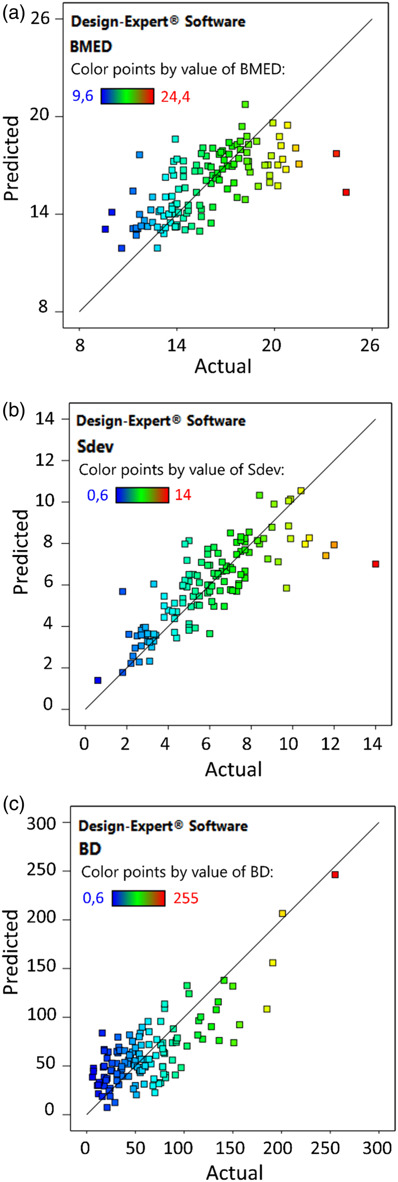

Target	Order	R²	Adj. R²	P-value whole-plot	P-value sub-plot	Most significant terms (p-value < 0.01)
BMED	Quartic	0.638	0.592	0.023	0.04	r², c.r.d²
Sdev	Quartic	0.692	0.656	0.029	0.008	r², d, d³
BD	Cubic	0.741	0.704	0.010	<0.0001	d, c.d, c².d, c.r², c.d², b.d²

Although high-order polynomials (above quadratic) are not usually used in RSM, they may provide more accurate predictions than low-order polynomials, as have been shown in previous works.^67–69 This may be because of the way the parameters affect the physical magnitudes and the overall complexity of the electrospinning process dynamics. Increasing the polynomial degree is generally associated with overfitting due to increasing degrees of freedom, however, this must be contrasted with other metrics and results. Analysis of variance (ANOVA) was utilized to test the significance of the model and factors. The p-value is a probability that measures the evidence against the null hypothesis; in this study, the null hypothesis is that the proposed model does not explain any of the variation in the response. Lower p-values provide stronger evidence against the null hypothesis, and therefore they support the hypothesis that the model does in fact explain the variations in the response. A significance level of 0.05 indicates a 5% risk of concluding that the model explains variation in the response when the model does not. In the same way, a predictor or factor that has a low p-value (<0.05) is more likely to be a meaningful addition to the model because changes in the predictor’s value are related to changes in the response variable. As can be seen in Table 4, p-values show the significance of the whole-plot (c, r and their interactions) and the sub-plot (rest of variables and interactions). The terms in the last column showed the highest statistical significance, having a p-value lower than 0.01.

The R² values in the range 0.63–0.74 imply that most of the variance in the response variables can be explained by the input variables. The remaining can be attributed to unknown (not considered) variables or inherent variability of the targets. The presence of some outliers can be seen in Figure 5, which adversely affect the model’s performance. The small differences between R² and adjusted R² imply that included terms are mainly significant to the model, which further supports a low probability of overfitting.

The most significant terms mainly correlate with the results of the correlation matrix (Figure 4(b)), where c and r have the highest Pearson coefficients, followed by d. This empirical model, however, does not pretend to explain an analytical relation between input and response variable, and therefore the higher-order terms do not necessarily imply a real physical relation between magnitudes.

This method proved to be a very fast and easy-to-use modeling tool. However, testing of different model approaches was needed to achieve the best possible model.

MLR study

Each model was optimized via cross-validation, and the hyper-parameters that minimized RMSE were found for each model (Table 5). Complete GridSearchCV results are shown in Supplemental Figure S2 in Supporting Information. The degrees of the RR polynomials for each target were 4, 6 and 3 respectively. Interestingly, the first and third values match with the degree of the RSM optimized polynomials. The 6-order polynomial of the Sdev model may be explained by the penalty parameter λ, which allows a higher number of degrees of freedom without overfitting.

Table 5.

Summary of MLR models performance in training and testing sets.

	BMED			Sdev			BD
	Hyper-parameters	RMSE train	RMSE test	Hyper-parameter	RMSE train	RMSE test	Hyper-parameters	RMSE train	RMSE test
RR	Degree = 4	1.78	1.84	Degree = 6	1.68	1.69	Degree = 3	27.9	26.8
RR	λ = 0.1			λ = 0.1			λ = 10
SVR	C = 10³	1.78	1.83	C = 10⁵	1.65	1.67	C = 10	26.3	25.0
	α = 0.1			α = 0.01			α = 10
RF	N = 500	1.79	1.85	N = 50	1.62	1.65	N = 300	27.6	27.3
	Depth = 3			Depth = 3			Depth = 1
VR	—	1.77	1.82	—	1.60	1.64	—	26.3	25.0

The VR ensemble was computed by combining the three previously optimized algorithms (for each target). Three approaches were considered for weighting the models: using the inverse of the RMSE as the weight, ranking the models from three to one according to the RMSE (highest rank to the lowest RMSE), and squaring the rank values. The last approach was the most successful, achieving the lowest RMSE for the VR models of each target. Table 5 shows that each algorithm performed best in a different target, but the VR outperformed the others in all three.

The similarity of the RMSE values in train and test sets shown in Table 5 confirms the excellent generalization of the model, achieved via cross-validation. The fact that in some cases the RMSE-test is slightly smaller than the RMSE-train, can be explained by the relatively small number of data points of the test-set (i.e. 32 vs 94): with almost three times the number of data points, the training set is more exposed to outliers and general variability of data that is not explained by the model. Furthermore, Figure 6 shows the predicted versus actual values for the VR model, where the presence of outliers is more notably in the training set. It is worth noticing that RMSE is a metric that, by construction, emphasizes the presence of outliers, in contrast with the mean absolute error. The computed p-value of the VR model was <0.001.

Figure 6.

Plots of the actual target values versus the predicted by the VR model. (a) BMED, (b) Sdev, (c) BD.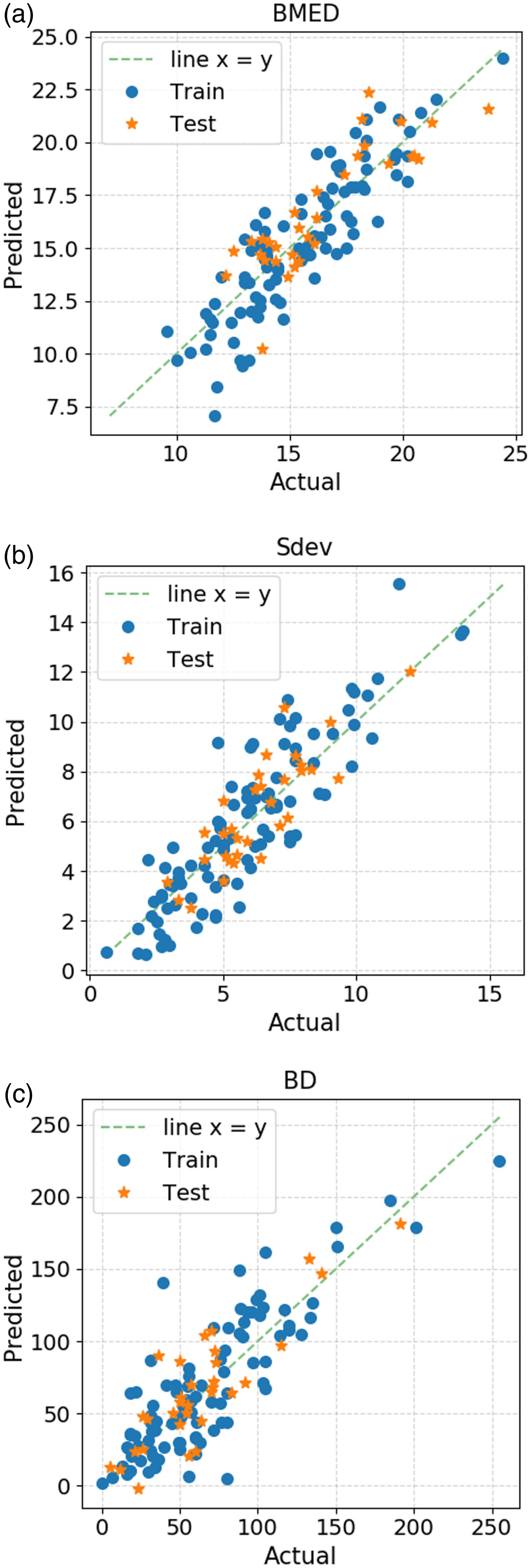

The permutation feature importance is defined to be the decrease in a model score when a single feature value is randomly shuffled. This way, the relative importance of each feature in the model was calculated for the VR model (Figure 7). The solvent ratio appears to be the single most relevant parameter for the BMED and Sdev, followed by polymer concentration. PVDF concentration has the most significant impact in BD, but it is closely followed by solvent ratio and tip-to-collector distance. This is in agreement with the findings of Desai et al., with the difference that in their study, a single solvent was used and therefore solvent weight ratio was not an input variable.⁷⁰ Analogously to the values found in the correlation matrix (Figure 4(b)), the voltage does not seem to be a relevant parameter for the models either.

Figure 7.

Importance of each feature in the VR model for (a) BMED, (b) Sdev, (c) BD.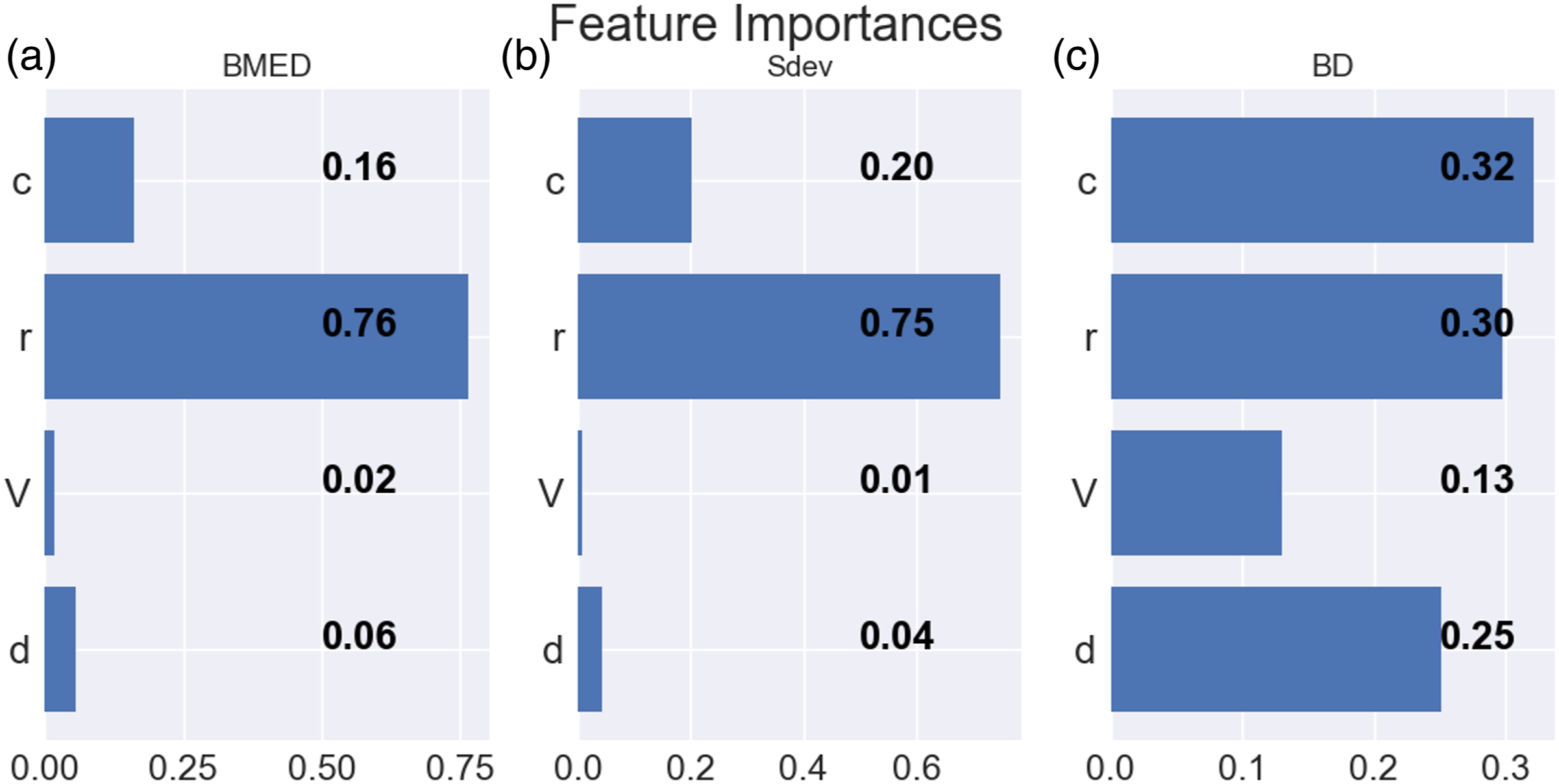

Model comparison

To compare the methods performances, RMSE and coefficient of determination of each model over the whole dataset are shown in Table 6. Machine learning regressions represented by the VR model performs better in every case.

Table 6.

RMSE and R² for each model.

	BMED		Sdev		BD
	RMSE	R²	RMSE	R²	RMSE	R²
RSM	2.17	0.638	1.85	0.692	27.9	0.741
VR	1.78	0.724	1.61	0.700	26.0	0.775

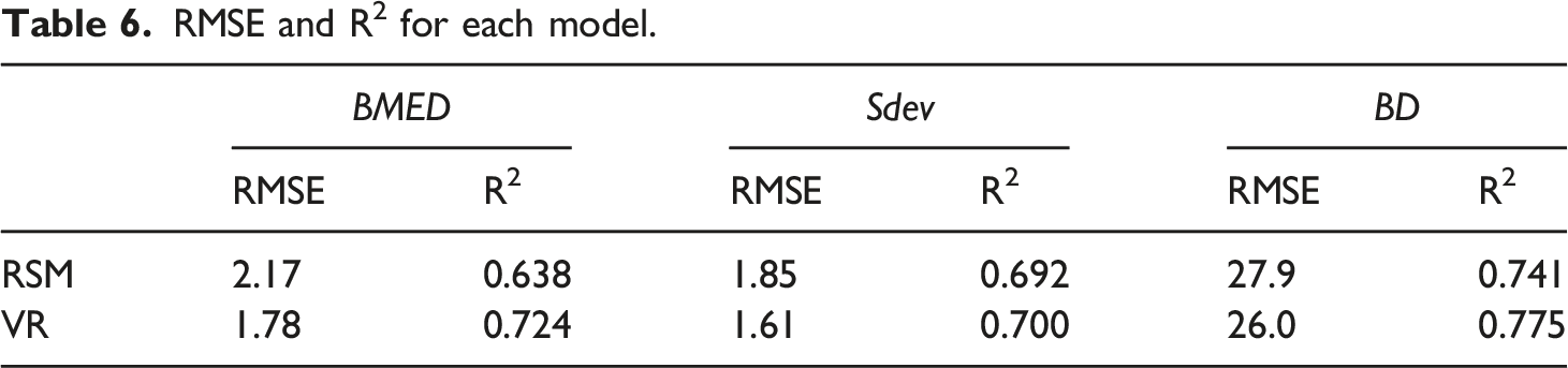
Figure 8 shows the 3D surface of the response variables as a function of PVDF concentration and solvent ratio, by fixing voltage and distance in the values that minimize each target (Table 7). The surfaces created by both methods follow similar trends, but the VR surface shows slightly more irregular curves as a result of the model ensemble. In particular, RF is composed of an assembly of discrete cuts, rather than smooth curves.

Figure 8.

3D Surface plots of the target optimized RSM models (a), (b), (c) and VR models (d), (e), (f) as a function of polymer concentration and solvent ratio. Voltage and tip-to-collector distance were fixed in the values that minimized each target.

Table 7.

Features values that minimize each target according to the RSM and VR models.

		c (wt%)	r (w/w)	V (kV)	d (cm)	Target value
BMED	RSM	19.7–20.0	2.80–2.90	8.0–8.8	35	7.6
BMED	VR	18.7	2.32	8.0	35	5.8
Sdev	RSM	19.7–19.85	2.37	8.0	35	0.75
Sdev	VR	19.3	2.55	8.0	35	0.56
BD	RSM	16.9	1.69	8.0–10	30	1.7
BD	VR	16.4	1.54	13	32	0.1

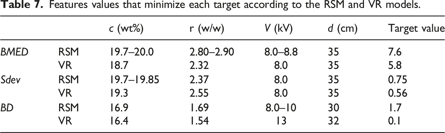
The parameters which minimize each target are shown in Table 7. Generally, both methods lead to similar feature values, but there are a few cases to consider. The BMED-RSM model has its minimum at the extreme values of c (20 wt%) and r (2.9 w/w), while the VR model has its minimum away from the borders of the c-r space (18.7 wt%, 2.32 w/w). Also, the BD models differ considerably in the optimal voltage. The VR model reaches lower values in all three targets.

Machine learning regressions models are not constraint by polynomials (except for the RR, that has also a regularization parameter) and so they can explore and adapt to very complex and multidimensional relations with a smaller number of parameters. This may explain the better performance of the MLR over the RSM.

Testing the predictions

To experimentally test the predictions of the models, two important cases were studied: bead-free fibers and minimum-sized beads. For the former, BD = 0 represents a mat with no beads, while for the latter, BMED must be minimized. Therefore, the BD and BMED parameters shown in Table 7 stand the highest probability of achieving each respective goal.

Figures 8(c) and (f) show the predictions of each model in the c – r parameter space by fixing V and d as in Table 7 for the minimum BD (8.0 kV–35 cm and 13 kV–32 cm respectively). Figures 8(a) and (d) show the analogous prediction surface but for mininum BMED (8.0 kV–35 cm).

Final experimental tests were made to verify the predicted values of the models. Figure 9 shows the fibers obtained for each predicted combination of parameters. Figures 9(a) and (b) show the samples obtained with the parameters that minimized BD for both models. The result BD = 0 confirms the predictions of both models (within small errors). Analogously, the BMED models predicted minimum values of 7.6 and 5.8 μm for the RSM and MLR optimized models respectively, while the encountered experimental values (Figures 9(c) and (d)) were 6.5 and 6.1 μm. Finally, the Sdev predicted versus actual values for the same parameters were 1.2 vs 1.4 for the RSM model and 0.8 vs 1.1 for the MLR model.

Figure 9.

Optic microscope images, and SEM images (insets) of the final experimental tests. (a) RSM, optimal BD parameter combination. (b) VR, optimal BD parameter combination. (c) RSM, minimum BMED parameter combination. (d) VR, minimum BMED parameter combination. (e) and (f) show the histograms of the BED distribution of the samples shown in figure (c) and (d) respectively.

The results show an excellent concordance between the experimental and modeled data, which verifies the predicting ability of the models and their usefulness to find the desired target value. Furthermore, the use of an ensemble model that combines the results of distinct algorithms, turned out to be a very effective way to improve model performance.

Overall, both methods led to satisfactory results, but MLR showed slightly better performance, predicting ability and a better way to avoid overfitting. These qualities may be more crucial in systems where the results vary more abruptly. However, MLR were much more time-consuming than RSM, mainly because of the coding time and secondly the computing times. The availability of the script created in this work here provided may resolve MLR’s biggest disadvantage for future works regarding electrospinning parameter optimization.

Influence of electrospinning parameters on bead formation

The parameter importance shown in Figure 7 leads to the conclusion that conductivity or charge density and surface tension, which are determined mainly by solvent ratio, are the most significant physical magnitudes regarding bead size. The viscosity of the solution, determined mainly by polymer concentration, is the second most significant parameter for bead diameter and standard deviation. Korycka et al. have concluded that viscosity plays the most important role in bead size, but their study consisted of a single solvent solution of PVP in ethanol.⁴⁸

Bead density is highly affected by polymer concentration, solvent ratio, and tip to collector distance as well, which supports the fact that bead formation depends strongly on the polymer solution properties but also on the complex electrospinning dynamics. The fact that polymer concentration is the most relevant factor in beads number (Figure 7) is in agreement with the works of Ruiter et al.²⁸, Khanlou et al.⁴⁷, and Cui et al.⁴⁶ The latter also reported the significance of the molecular weight and solvent system. Zaarour et al. showed that the formation of beads-on-string structures in PVDF electrospinning is highly dependent on solvent system, solvent ratio and polymer concentration.³⁷

It is well known that there is a minimum polymer concentration for the formation of fibers by electrospinning and that below that value, only beads are obtained.^14,71,72 This is because it is necessary to overcome the concentration of interchain entanglement to avoid capillary breakage. In that sense, the formation of beads and bead-on-string structures is often related to low concentration. However, in this work, the range of concentrations is outside that regime (>15%), so the relation between polymer concentration and number of beads is not monotonic. In fact, solution viscosity also plays a role in restraining jet stretching and may lead to beads and thicker fibers. In this study, bead-free fibers were obtained with PVDF concentrations between 16.4 and 16.9 wt%, while by increasing polymer concentration, bead-on-string fibers were obtained. This is similar to the recent findings of Song et al., who made PVDF (M_w = 534 kDa) fibers by the similar technique of near-field electrospinning and obtained smooth bead-free fibers for 16–18 wt% concentrations, and beads-on-string structures above 18 wt%. Moreover, it is important to notice that the range of functional polymer concentration for electrospinning will be correlated with the molecular weight (M_w) of the polymer, as higher M_w increases chain entanglements and viscosity.³⁵ Supplemental Figure S3 (Supporting Info) shows the relation between optimized DMAC/acetone electrospinning solution concentration and PVDF molecular weight found in other studies. It clearly shows that the polymer concentration which leads to bead-free mats is inversely correlated with M_w.

Low conductivity and high surface tension are associated with bead formation, as the electrical forces may result insufficient to elongate the jet and produce uniform fibers.^14,73 As shown in Table 1, DMAC has much higher conductivity than acetone, but higher surface tension as well. Both magnitudes play an opposite role in the fiber-bead formation dynamic. According to Figures 4(b) and 8, DMAC/acetone ratio seems to generally reduce the size and size dispersion of beads but increase its number.

Finally, Figure 10 shows the response surface of the VR model in the V-d space. Increasing the distance between tip and collector seems to generally reduce the values of the three targets (also in accordance to Figure 4(b)), tending to the formation of small and regular beads or bead-free mats. This may be related to the stretching of the jets by enlarging its instability region.¹⁵ The effect of the voltage varies depending on the distance, so no general trend can be stated. However, lower V values seem to reduce bead size and size dispersion for large distances. Voltage is the least significant parameter according to both models, but it should be noticed that the parameter range for V is 100% (from 8 to 16 kV) while for d is 350% (from 10 to 35 cm).

Figure 10.

3D Surface plots of the VR optimized models as a function of voltage and distance. The PVDF concentration and DMAC/acetone ratio were fixed in the values that minimized each target.

Conclusions

Response surface methodology and machine learning regressions models were successfully able to predict the relation between electrospinning parameters and bead-size and bead density on PVDF electrospun mats with a small number of tests. Both models were able to find the combination of parameters that lead to bead-free mats and minimum sized beads.

Response surface methodology quartic and cubic models showed significance through low p-values (<0.05) and reasonable R² and adjusted R² values. Despite the high order polynomials, the model did not overfit the data.

Machine learning regressions achieved lower RMSE and higher R² values than RSM, and the VR ensemble resulted in an effective meta-model, outperforming the individual regressions. The training through cross-validation is a very effective way to avoid overfitting and achieve good generalization ability, which was verified by the similitude between train and test RMSE values.

The PVDF concentration and DMAC/acetone ratio were the most influential parameters of the bead formation process. The results presented herein support the inverse correlation between molecular weight and optimal polymer concentration for bead-free mats. For low bead size and size variance, the optimal parameters were 18.7 wt% polymer concentration, 2.32 w/w DMAC/acetone ratio, 8.0 kV and 35 cm. To minimize the bead density and obtain bead-free mats, the optimal parameters were 16.4 wt%, 1.54 w/w DMAC/acetone ratio, 13 kV and 32 cm.

Overall, RSM via Design Expert resulted a much faster method, but the MLR achieved better performance, versatility and showed useful tools for its optimization. The availability of the python script provided by this work may help other groups significantly reduce the coding time necessary to implement this method to predict electrospinning response variables. This work may help introduce highly efficient predicting algorithms into electrospinning research, greatly reducing the time needed to obtain optimal morphology for any polymer-solvent system and electrospinning machine.

Supplemental Material

Supplemental Material - A prospective randomised comparative study of dynamic, static progressive and serial static proximal interphalangeal joint extension orthoses

Supplemental Material for Poly(vinylidene fluoride) electrospun nonwovens morphology: Prediction and optimization of the size and number of beads on fibers through response surface methodology and machine learning regressions by Federico Javier Trupp, Roberto Cibils and Silvia Goyanes in Journal of Industrial Textiles

Footnotes

Declaration of Conflicting Interests

The author(s) declared no potential conflicts of interest with respect to the research, authorship, and/or publication of this article.

Funding

The author(s) disclosed receipt of the following financial support for the research, authorship, and/or publication of this article: This work was supported by the Fondo para la Investigación Científica y Tecnológica (PICT 2017-2362).

ORCID iD

Silvia Goyanes

Supplemental Material

Supplemental material for this article is available online.

References

Saber

Abd El-Aziz

. Advanced materials used in wearable health care devices and medical textiles in the battle against coronavirus (COVID-19): a review. J Ind Text 2021; 15280837211041771.

Sanyal

Sinha-Ray

. Ultrafine PVDF nanofibers for filtration of air-borne particulate matters: a comprehensive review. Polymers (Basel) 2021; 13: 1864.

Zaarour

Tina

Zhu

, et al. Branched nanofibers with tiny diameters for air filtration via one-step electrospinning. J Ind Text 2020; 152808372092377.

Akduman

. Cellulose acetate and polyvinylidene fluoride nanofiber mats for N95 respirators. J Ind Text 2021; 50: 1239–1261.

Zhu

Zaarour

Jin

. Unexpectedly high oil cleanup capacity of electrospun poly (vinylidene fluoride) fiber webs induced by spindle porous bowl like beads. Soft Mater 2019; 17: 410–417.

Cimadoro

Goyanes

. Reversible swelling as a strategy in the development of smart membranes from electrospun polyvinyl alcohol nanofiber mats. J Polym Sci 2020; 58: 737–746.

Pereira

Fernandez

Cimadoro

, et al. Biohybrid membranes for effective bacterial vehiculation and simultaneous removal of hexavalent chromium (CrVI) and phenol. Appl Microbiol Biotechnol 2021; 105: 827–838.

Torasso

Vergara-Rubio

Rivas-Rojas

, et al. Enhancing arsenic adsorption via excellent dispersion of iron oxide nanoparticles inside poly(vinyl alcohol) nanofibers. J Environ Chem Eng 2021; 9: 104664.

López-Córdoba

Castro

Goyanes

. A simple green route to obtain poly(vinyl alcohol) electrospun mats with improved water stability for use as potential carriers of drugs. Mater Sci Eng C 2016; 69: 726–732.

10.

Wang

Huang

Liu

, et al. Poloxamer188 composite electrospun poly L-lactic acid fibrous nonwoven: sustained in vitro and in vivo release letrozole as a subcutaneous implant. J Ind Text 2022; 152808372110620.

11.

Ranjbar-Mohammadi

Nouri

. Production and in vitro analysis of catechin incorporated electrospun gelatin/poly (lactic acid) microfibers for wound dressing applications. J Ind Text 2021; 1–16.

12.

Islam

Ang

Andriyana

, et al. A review on fabrication of nanofibers via electrospinning and their applications. SN Appl Sci 2019; 1: 1248.

13.

Zuo

Zhu

Yang

, et al. Experimental study on relationship between jet instability and formation of beaded fibers during electrospinning. Polym Eng Sci 2005; 45: 704–709.

14.

Fong

Chun

Reneker

. Beaded nanofibers formed during electrospinning. Polymer (Guildf) 1999; 40: 4585–4592.

15.

Duque Sánchez

Rodriguez

López

. Electrospinning: the nanofibers age. Rev Iberoam Polímeros Vol Iber Polímeros 2014; 14: 10–27.

16.

Ribba

Parisi

D’Accorso

, et al. Electrospun nanofibrous mats: from vascular repair to osteointegration. J Biomed Nanotechnol 2014; 10: 3508–3535.

17.

Cui

, et al. Multistructured electrospun nanofibers for air filtration: a review. ACS Appl Mater Inter 2021; 13: 23293–23313.

18.

Yun

Suryamas

Iskandar

, et al. Morphology optimization of polymer nanofiber for applications in aerosol particle filtration. Sep Purif Technol 2010; 75: 340–345.

19.

Kadam

Kyratzis

Truong

, et al. Electrospun bilayer nanomembrane with hierarchical placement of bead-on-string and fibers for low resistance respiratory air filtration. Sep Purif Technol 2019; 224: 247–254.

20.

Cao

Meng

Tan

, et al. Electrospun bead-in-string fibrous membrane prepared from polysilsesquioxane-immobilising poly(lactic acid) with low filtration resistance for air filtration. J Polym Res 2020; 27: 5.

21.

Zhang

Yang

, et al. Nanofibrous membrane of graphene oxide-in-polyacrylonitrile composite with low filtration resistance for the effective capture of PM2.5. J Memb Sci 2018; 551: 85–92.

22.

Matulevicius

Kliucininkas

Prasauskas

, et al. The comparative study of aerosol filtration by electrospun polyamide, polyvinyl acetate, polyacrylonitrile and cellulose acetate nanofiber media. J Aerosol Sci 2015; 92: 27–37.

23.

Rajak

Hapidin

Iskandar

, et al. Controlled morphology of electrospun nanofibers from waste expanded polystyrene for aerosol filtration. Nanotechnology 2019; 30: 5602.

24.

Huang

Tian

Wang

, et al. Fabrication of bead-on-string polyacrylonitrile nanofibrous air filters with superior filtration efficiency and ultralow pressure drop. Sep Purif Technol 2020: 237: 116377.

25.

Greenfeld

Rodricks

Sui

, et al. Beaded fiber composites—Stiffness and strength modeling. J Mech Phys Sol Beaded Fiber Composites — Stiffness Strength Modeling 2019; 125: 384–400.

26.

Lee

Park

. Highly hydrophobic nanofibrous surfaces genearated by poly(vinylidene fluoride). Fibers Polym 2013; 14: 1271–1275.

27.

Xue

Guo

Zhou

, et al. Influence of beads-on-string on Na-Ion storage behaviors of electrospun carbon nanofibers. Carbon N Y 2019; 154: 219–229.

28.

Ruiter

FAA

Alexander

Rose

FRAJ

, et al. A design of experiments approach to identify the influencing parameters that determine poly-D,L-lactic acid (PDLLA) electrospun scaffold morphologies. Biomed Mater 2017; 12: 055009.

29.

Kim

Choi

, et al. Electrospun PVdF-based fibrous polymer electrolytes for lithium ion polymer batteries. Electrochim Acta 2004; 50: 69–75.

30.

Hwang

Kwon

Byun

. Preparation of PVdF nanofiber membranes by electrospinning and their use as secondary battery separators. J Memb Sci 2011; 378: 111–116.

31.

Yang

, et al. Hydrophobic polyvinylidene fluoride fibrous membranes with simultaneously water/windproof and breathable performance. RSC Adv 2016; 6: 87820–87827.

32.

Yang

, et al. Influence of working temperature on the formation of electrospun polymer nanofibers. Nanoscale Res Lett 2017; 12: 55. Epub ahead of print 2017. DOI: 10.1186/s11671-016-1824-8

33.

Shim

Kouh

. Effects of electrospinning nozzle size and voltage on polyvinylpyrrolidone fiber structure formation. New Phys Sae Mulli 2020; 70: 531–534.

34.

Szewczyk

Stachewicz

. The impact of relative humidity on electrospun polymer fibers: From structural changes to fiber morphology. Adv Colloid Interf Sci 2020; 286: 102315.

35.

Nayak

Ghosh

Bhatnagar

. Investigation of solution rheology in electrospinning of ultra high molecular weight polyethylene. Fibers Polym 2021; 23: 48–57.

36.

Guerreiro

SFC

Valente

JFA

Dias

, et al. Box-Behnken design a key tool to achieve optimized PCL/gelatin electrospun mesh. Macromol Mater Eng 2021; 306: 2000678.

37.

Zaarour

Zhang

Zhu

, et al. Maneuvering surface structures of polyvinylidene fluoride nanofibers by controlling solvent systems and polymer concentration. Text Res J 2019; 89: 2406–2422.

38.

Zaarour

Zhu

Jin

. Maneuvering the secondary surface morphology of electrospun poly (vinylidene fluoride) nanofibers by controlling the processing parameters. Mater Res Express 2019; 7: 015008.

39.

Zaarour

Zhu

Jin

. A review on the secondary surface morphology of electrospun nanofibers: formation mechanisms, characterizations, and applications. ChemistrySelect 2020; 5: 1335–1348.

40.

Weichert

Link

Stoll

, et al. A review of machine learning for the optimization of production processes. Int J Adv Manuf Technol 2019; 104: 1889–1902.

41.

Marques

Prates

Pereira

AFG

, et al. Performance comparison of parametric and non-parametric regression models for uncertainty analysis of sheet metal forming processes. Metals (Basel) 2020; 10(4), 457.

42.

Nasouri

Shoushtari

Mojtahedi

MRM

. Evaluation of effective electrospinning parameters controlling polyvinylpyrrolidone nanofibers surface morphology via response surface methodology. Fibers Polym 2015; 16: 1941–1954.

43.

Kheirkhah Barzoki

Latifi

Rezadoust

. Response surface methodology optimization of electrospinning process parameters to fabricate aligned polyvinyl butyral nanofibers for interlaminar toughening of phenolic-based composite laminates. J Ind Text 2020; 49: 858–874.

44.

Chomachayi

Solouk

Mirzadeh

. Mathematical modeling of electrospinning process of silk fibroin/gelatin nanofibrous mat: comparison of the accuracy of GMDH and RSM models. J Ind Text 2021; 50: 1020–1039.

45.

Angel

Guo

Yan

, et al. Effect of processing parameters on the electrospinning of cellulose acetate studied by response surface methodology. J Agric Food Res 2020; 2: 100015.

46.

Cui

Zhou

, et al. Investigation on process parameters of electrospinning system through orthogonal experiment design. J Appl Polym Sci 2007; 103: 3105–3112.

47.

Khanlou

Ang

Talebian

, et al. Multi-response analysis in the processing of poly (methyl methacrylate) nano-fibres membrane by electrospinning based on response surface methodology: fibre diameter and bead formation. Meas J Int Meas Confed 2015; 65: 193–206.

48.

Korycka

Mirek

Kramek-Romanowska

, et al. Effect of electrospinning process variables on the size of polymer fibers and bead-on-string structures established with a 23 factorial design. Beilstein J Nanotechnol 2018; 9: 2466–2478.

49.

Hassan

, et al. Effective modeling and optimization of PVDF–PTFE electrospinning parameters and membrane distillation process by response surface methodology. J Appl Polym Sci 2019; 136: 1–12.

50.

Naghibzadeh

Adabi

. Evaluation of effective electrospinning parameters controlling gelatin nanofibers diameter via modelling artificial neural networks. Fibers Polym 2014; 15: 767–777.

51.

Rabbi

Nasouri

Bahrambeygi

, et al. RSM and ANN approaches for modeling and optimizing of electrospun polyurethane nanofibers morphology. Fibers Polym 2012; 13: 1007–1014.

52.

Nasouri

Bahrambeygi

Rabbi

, et al. Modeling and optimization of electrospun PAN nanofiber diameter using response surface methodology and artificial neural networks. J Appl Polym Sci 2012; 126: 127–135.

53.

Nurwaha

Wang

. Modeling and optimization of electrospun PAN nanofiber diameter using response surface methodology and artificial neural networks. Glob J Technol Optim 2019; 10: 1–6.

54.

Wang

Cai

Liu

, et al. Harnessing a novel machine-learning-assisted evolutionary algorithm to co-optimize three characteristics of an electrospun oil sorbent. ACS Appl Mater Inter 2020; 12: 42842–42849.

55.

Toscano

Segura

, et al. A machine leraning approach fo model the electrospinning process of biocompatible materials. In: Manufacturing Science and Engineering Confrerence MSEC2020, 22–26 June 2020, Cincinnati, OH, USA, 2020, pp. 1–9.

56.

Ieracitano

Paviglianiti

Campolo

, et al. A novel automatic classification system based on hybrid unsupervised and supervised machine learning for electrospun nanofibers. IEEE/CAA J Autom Sin 2021; 8: 64–76.

57.

Jones

Goos

. I-Optimal versus D-Optimal split-plot response surface designs. J Qual Technol 2012; 44: 85–101.

58.

Gong

Wang

, et al. A high-strength PPESK/PVDF fibrous membrane prepared by coaxial electrospinning for lithium-ion battery separator. High Perform Polym 2019; 31: 948–958.

59.

Buddhakala

Muakngam

. Preparation of Poly(Vinylidene Fluoride)/silica composite nanofiber by electrospinning technique. Appl Mech Mater 2015; 804: 84–87.

60.

Kim

J-W

Kim

D-G

Koo

J-M

, et al. Characterization of failure behaviors in anisotropic conductive interconnection. Mater Trans 2007; 48: 1070–1078.

61.

Moshfeghian

Azimi

Mahkam

, et al. Effect of solution properties on electrospinning of polymer nanofibers: a study on fabrication of PVDF nanofibers by electrospinning in DMAC and (DMAC/Acetone) solvents. DormajOrg 2021; 2: 53–58.

62.

Damaraju

Jaffe

, et al. Structural changes in PVDF fibers due to electrospinning and its effect on biological function. Biomed Mater 2013; 8: 045007.

63.

Anderson

Whitcomb

. RSM simplified – optimizing process using response surface methods for design of experiments. New York, NY, USA: Productivity Press, 2004. Epub ahead of print 2004. DOI: 10.4324/9781482293777

64.

Friedman

Hastie

Tibshirani

. The elements of statistical learning data mining, interface and prediction preface to the second edition. New York, NY: Springer, 2009, p. 809.

65.

Shmilovici

. Support vector machines. In: Maimon

Rokach

(eds) Data mining and knowledge discovery handbook. New York, NY, USA: Springer, 2005, pp. 257–276.

66.

Polikar

. Ensemble learning. In: Zhang

(eds) Ensemble machine learning. Boston, MA: Springer, 2012, pp. 1–34.

67.

de Souza

Alavarse

da Vinci

, et al. The synergistic effect of polymer composition, solvent volatility, and collector distance on pullulan and PVA fiber production by rotary jet spinning. Fibers Polym 2021; 22: 942–956.

68.

Hong

Harker

Edirisinghe

. Empirical modelling and optimization of pressure-coupled infusion gyration parameters for the nanofibre fabrication.pdf. Proc R Soc A 2019; 475: (2225): 20190008.

69.

Doustgani

Vasheghani-Farahani

Soleimani

, et al. Optimizing the mechanical properties of electrospun polycaprolactone and nanohydroxyapatite composite nanofibers. Compos B Eng 2012; 43: 1830–1836.

70.

Desai

Sung

. DOE optimization and phase morphology of electrospun nanofibers of PANI/PMMA blends electrospinning set-up. NSTI-nanotech 2004; 3: 429–432.

71.

Eda

Shivkumar

. Bead-to-fiber transition in electrospun polystyrene. J Appl Polym Sci 2007; 106: 475–487.

72.

Casasola

Thomas

Georgiadou

. Electrospinning of poly(lactic acid): Theoretical approach for the solvent selection to produce defect-free nanofibers. J Polym Sci B Polym Phys 2016; 54: 1483–1498.

73.

Haghi

. Electrospinning of nanofibers in textiles. Boca Ratón, FL, USA: CRC Press, 2012. Epub ahead of print 2012. DOI: 10.1201/b12229

Supplementary Material

Please find the following supplemental material available below.

For Open Access articles published under a Creative Commons License, all supplemental material carries the same license as the article it is associated with.

For non-Open Access articles published, all supplemental material carries a non-exclusive license, and permission requests for re-use of supplemental material or any part of supplemental material shall be sent directly to the copyright owner as specified in the copyright notice associated with the article.

0.00 MB

0.53 MB