Sage Journals: Discover world-class research

Abstract

In the past two decades, a number of models have been built to simulate the motion of polymer jet during melt blowing. Unfortunately, the complex interaction between polymer jet and air flow field has been rarely reported. In this work, a phase-field method was applied to simulate the coupling effects between polymer and air flow during melt blowing and the computed results were compared with the results of the model built through level-set method and experimental results. Velocity in the x direction, velocity in the y direction, whipping amplitude and diameter of polymer jet were discussed, respectively. It was found that the velocity predicted by the present model was higher than that predicted by the level-set method. However, both of them are close to the experimental value. The calculated final fiber diameter based on the phase-field method is much closer with the experimental value than that based on the level set method. Based on the model, the effect of polymer surface tension and slot angle on the polymer jet velocity were discussed.

Keywords

Phase-field method melt blowing coupled model polymer jet velocity two-phase flow

Introduction

Melt blowing is a one-step process for converting polymeric raw materials into ultrafine fiber nonwovens. During melt blowing, the polymer melt is extruded through small holes into converging high-speed hot air streams, and attenuated by the drag force of air until reach the collector positioned some distance away from the melt-blowing die, as depicted in Figure 1. Due to its small fiber diameter, melt blown nonwovens find applications in a variety of areas such as filtration, sorbent, and insulation [1].

Figure 1.

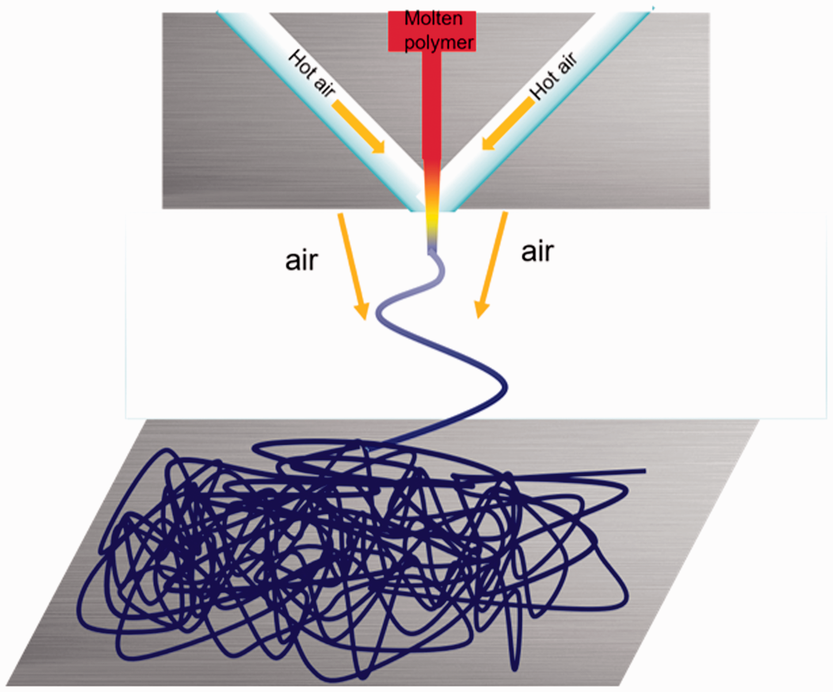
Schematic of the melt blowing process.

In the melt blowing process, the key flow element is a polymeric liquid jet stretched by a high speed gas flow. The motion of melt blown polymer jet, which influences the properties of final product, has always been an interest of the researchers. However, the motion of the polymer jet, especially the velocity is difficult to measure directly. The work of Uyttendaele and Shambaugh firstly introduced the photography technique to acquire the jet velocity during melt blowing [2].

In their method, the velocity was obtained based on the jet diameter measured from the photographing image and the law of mass conservation. However, due to the limitation of photographic technology in 1990, the images tend to be blurred when the jet velocity is increased. Thus, the air velocity adopted in their experiment was low (17–55 m/s) [3]. For the polymer jets in a relatively higher air velocity (90 m/s), Laser Doppler Velocimeter (LDV) is a better option to investigate the velocity. Wu and Shambaugh [4] examined the jet velocities in three-dimensional space with LDV.

Bresee and his coworkers [3,5,6] measured the jet velocity by analyzing triple-exposed images obtained with the high speed camera and high pulsed laser. The jet velocity was obtained according to the laser pulse separation time and jet moving distance during the interval time. They claimed that the air pressure of the machine in their research was supplied at a commercial condition. Unfortunately, the photographing images they offered did not show the jet whipping during melt blowing.

Beard et al. [7] captured the melt blown jet whipping for the first time with 2000 frame/s photographing speed. However, the successive images of the jet motion and the discussion of jet velocity were not presented in their work. With high-speed camera working at frame rate of 5000 frame/s, the previous work of our group [8] recorded the melt blown jet path. Based on the images recorded, the jet whipping and velocity were measured.

Since the measurement of the jet velocity is time and cost consuming, and is limited by the processing and measuring conditions. Numerical method has been the alternative option to the experimental measurement to acquire the jet motion information during melt blowing. Uyttendaele and Shambaugh [2] firstly carried out the modelling work of melt blown polymer jet. In their model, the motion of polymer jet was assumed to be one-dimensional. After that, Rao and Shambaugh [9] and Marla and Shambaugh [10] conducted two-dimensional and three-dimensional modelling work, respectively. Besides, Chen and Huang [11], Zeng et al. [12], Jarecki and Ziabicki [13] and Sun et al. [14] also have done a great deal of work regarding the modelling of the melt blown jet motion. However, their numerical results of jet velocities were all underpredicted comparing with the experimental data available [5,15]. One of the reasons for the underprediction could be the negligence of the interaction between the polymer and the air in their models.

It is known that the process of melt blowing involves a complex interplay of the aerodynamics of air flow with polymer jets. Therefore, the coupling of the air flow with the polymer can have a significant effect on the formation of melt blown fibers. In our previous study, a level-set method has been applied to simulate the air-polymer coupling effect during melt blowing, and the gap between simulation value and experimental value has been reduced [16]. In the present work, a method called phase-field has been employed to establish the air-polymer coupled model during melt blowing. The phase field method, not only convects the fluid interface with the flow field, but it also ensures that the total energy of the system diminishes correctly. In the present model, the mixing energy of two immiscible fluids is included, which was not considered in our previous model established by level set method. The computed results of the present model were compared with that from the level set method, and the experimental value for verification. The model construction, mesh generation and solving were all performed in Comsol Multiphysics.

Model construction

Geometry

A one-orifice slot die with a blunt nosepiece is employed in our research. Figure 2 shows the cross-sectional view and top view of the die studied. The dimensions of the die are listed in Table 1.

Figure 2.

Geometry of the die. (a) Section view, (b) top view.

Table 1.

Dimensions of the die.

Geometric parameters	Value
Nose-piece width (f)	1.28 mm
Slot angle (α)	60^。
Slot width (e)	0.65 mm
Slot length (l)	6 mm
Orifice diameter (d)	0.42 mm

Figure 3 depicts the computational domain for the model in this study. For the slot die, the air flow is supplied in the form of two converging high speed air jets. Previous researches indicate that the z-component velocity of the air jets is negligible, therefore the motion of the polymer jet in the neighbouring area of the die is mainly in the x-y plane [17]. In view of the information above-mentioned, the computational domain of this model is set to be two dimensional. The main domain for computation is a rectangular area with the size of 30 mm in the x-direction and 50 mm in the y-direction. Previous research found that most of the attenuation and acceleration of polymer jet occur within 2 cm from the die [18 –20]. Therefore, the computation domain is large enough for the study of polymer jet velocity under the die.

Figure 3.

Computation domain and boundary conditions of the model.

Governing equations

In the Phase Field method, the fluid interface separating the immiscible phases is tracked by a Cahn-Hilliard equation. Here, the fluid interface is the region where the dimensionless phase field variable (Φ) goes from -1 to 1. The Cahn-Hilliard equation is split up into two equations (1) and (2)

\frac{\partial \emptyset}{\partial t} + u \cdot \nabla \emptyset = \nabla \cdot \frac{γ λ}{ε^{2}} \nabla Ψ

(1)

Ψ = - \nabla \cdot ε^{2} \nabla \emptyset + (\emptyset^{2} - 1) \emptyset

(2)

Where t is time for the fluid motion (s), 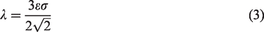u is the fluid velocity (m/s), γ is the mobility (m³s/kg), λ refers to the mixing energy density (N) and ε(m) is the measure of interface thickness. Equation (3) relates the mixing energy density and the interface thickness to the surface tension coefficient ( $σ$ ) which is set to be 0.02 N/m [21]

λ = \frac{3 ε σ}{2 \sqrt{2}}

(3)

The interface thickness parameter is set to be h_c/2, where hc is the characteristic mesh size in the region passed by the interface. The mobility parameter determines the time scale required by the Cahn-Hilliard diffusion and must be large enough to retain a constant interfacial thickness, while small enough so that the convective terms are not overly damped. In Comsol Multiphysics the mobility parameter is a function of the interface thickness, as described in equation (4)

γ = χ ε^{2}

(4)

Where $χ$ controls the mobility of the interface, it is set to be 1.

In the present model, the volume faction of polymer jet is defined by equation (5), and equation (6) is for air flow

V_{f 1} = \frac{1 - \emptyset}{2}

(5)

V_{f 2} = \frac{1 + \emptyset}{2}

(6)

The density (kg/m³) and the viscosity (Pa·s) of the mixture varying smoothly over the interface are defined by equations (7) and (8), respectively

ρ = ρ_{air} + (ρ_{poly} - ρ_{air}) V_{f 2}

(7)

μ = μ_{air} + (μ_{poly} - μ_{air}) V_{f 2}

(8)

Where parameters ρ, ρ_air and ρ_poly are density of the fluid mixture, air flow and polymer jet, respectively. The parameters μ, μ_air, μ_pol are dynamic viscosity of the fluid mixture, air flow and polymer jet, respectively.

The transport of momentum and mass are described in equations (9) and (10), respectively

ρ \frac{\partial u}{\partial t} + ρ (u \cdot \nabla) u = - \nabla p + \nabla \cdot [(μ + μ_{T}) (\nabla u + {(\nabla u)}^{T})] + F_{st} + ρ g

(9)

\frac{\partial ρ}{\partial t} + \nabla \cdot (ρ u) = 0

(10)

Where p is pressure of the fluid, μ_T is the turbulence viscosity, g is gravity acceleration, F_st is the surface tension force acting at the air/polymer interface. The surface tension force can be derived from equation (11)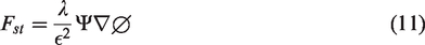

F_{s t} = \frac{λ}{ϵ^{2}} Ψ \nabla \emptyset

(11)

The high speed air flow filed of the melt blowing process is turbulent. The common turbulence model k–ω is applied as a closure for the Reynolds-averaged Navier-Stokes equations (9) and (10). The K- $ω$ model takes the form shown below

ρ \frac{\partial k}{\partial t} + ρ (u \cdot \nabla) k = \nabla \cdot ⌊(μ + μ_{T} σ_{k}^{*}) \nabla k⌋ + P_{k} - β_{0}^{*} ρ ω k

(12)

ρ \frac{\partial ω}{\partial t} + ρ (u \cdot \nabla) ω = \nabla \cdot [(μ + μ_{T} σ_{ω}) \nabla ω] + α \frac{ω}{k} P_{k} - ρ β_{0} ω^{2}

(13)

Where k is turbulence kinetic energy, $ω$ is specific dissipation rate, P_k is production term. The turbulence model parameters $α, σ_{k}^{*}, σ_{ω}, {β_{o}, β}_{o}^{*}$ are set to be 0.52, 0.5, 0.5, 0.072, 0.09, respectively.

Boundary conditions and mesh generation

As shown in Figure 3, the inlet for air flow entering the computational domain was defined as a velocity inlet of air with temperature of 260 °C. The right, left and the bottom boundaries were all set as pressure outlets with ambient pressure of 0 Pa and temperature of 20 °C. The inlet where polymer flow entering the computational domain was defined as a velocity inlet of polymer. The polymer exit where the polymer meet the air, was defined as initial interface. The other boundaries including the die face and internal surface of the slot, were set as wall with temperature of 260 °C.

The computational domain was discretizd into quadrilateral elements. To improve the computation accuracy of the area where polymer jet goes through, we have refined the mesh in this area. In order to find the optimal meshing strategy, three different grid schemes: 17,114 (Grid 1), 21,026 (Grid 2), and 25,394 (Grid 3) cells were contrasted. The polymer jet velocity distribution computed with the three different grid schemes were presented in Figure 4. It is observed that little difference is shown in the three schemes. Hence, in consideration of computational efficiency, Grid 1 is adopted in the subsequent computations.

Figure 4.

Comparison of polymer jet velocity for the three different grid schemes.

Verification method

In our previous study [16], we have conducted the observation of polymer jet motion on a one-orifice laboratory-scale melt-blowing device. The die equipped in the machine has the configuration depicted in Figure 2(a) and (b). A high-speed camera (i-speed 7, iX Inc., UK) was employed to monitor the polymer jet motion. The camera was equipped with a Tokina AT-X M100 PRO D 100 mm f 2.8 zoom lens (Kenko Tokina Co. Ltd., Japan). During the photographing, the camera was put in the direction that the axis of the camera lens was parallel with the slots (i.e. the z-direction). Figure 5 depicts one of the captured images of the polymer jet. The polymer used for producing melt blown fibers was 1100-melt-flow-rate polypropylene (SK, Seoul, Korea) with dynamic viscosity about 8 Pa·s at 260 °C. During the experiments, the polymer flow rate is 1.5 cc/min, polymer temperature and air temperature are both 260 °C. Two air flow rates of 30 and 40 slm (standard L/min) are used. In this paper, the polymer flow rate and air flow rate are discussed in the form of volume rate, the corresponding flow velocities are listed in Table 2.

Figure 5.

High-speed photographing image of the polymer jet.

Table 2.

Flow rate of air and polymer in the form of flow velocity and volume-flow rate.

	Flow velocity	Volume-flow rate
Air	73.8 m/s	30 slm
Air	98.4 m/s	40 slm
Polymer	0.181 m/s	1.5 cc/min

Results and discussion

Flow characteristics of polymer jet

Figure 6(a) depicts the velocity magnitude distribution of the two dimensional flow field. In Figure 6(b), the air velocity is filtered out using the post-processing tool of Comsol Multiphysics, therefore the velocity distribution and path of the polymer jet could be presented. It is observed that the polymer jet is accelerated rapidly (the magnitude color changes from blue to red) in a few millimeters after extruded from the capillary exit and then decreases slowly until reach the bottom boundary (the magnitude color changes from red to yellow).

Figure 6.

Contour of the velocity field with air flow rate of 40 slm, polymer flow rate of 1.5 cc/min and polymer dynamic viscosity of 8 Pa·s. (a) velocity field of the air-polymer jet mixture, (b) velocity field of polymer jet.

In Figure 7, a comparison between velocity in the y- direction ( $V_{y}$ ) and velocity in the x- direction ( $V_{x}$ ) is made. It is observed that $V_{y}$ is much higher than $V_{x}$ and they are varying in different patterns in the region our model covered. In the distance of several millimeters from die, $V_{y}$ increases to its maximum (54 m/s) rapidly from its initial velocity (0.18 m/s), and then gently decreases to 13.5 m/s within the distance of 50 mm. $V_{x}$ fluctuates around 0: the positive value means the polymer jet moves toward the right direction and the negative values means the polymer jet moves toward the left direction.

Figure 7.

Comparison of $V_{y}$ and $V_{x}$ along flow direction. The origin is the center of the die.

Whipping motion of polymer jet

The whipping motion can also be seen in the polymer jet path in Figure 6(b). After moving a short distance (about 20 mm) from the capillary exit in die nosepiece, jet whipping appears in the x-y plane. Figure 8 provides the evolution of the polymer jet whipping with time and it is shown that the motion of the polymer jet is changing with time. To investigate the whipping amplitude, we have overlapped 15 images of polymer jet at different times, as presented in Figure 9. Due to the fact that the polymer jet is deviating to one side, the resultant overlapped polymer jet is not showing a cone as previous studies described [8,22]. However, the result is still acceptable as a reference.

Figure 8.

The evolution of polymer jet motion during melt blowing with air flow rate of 40 slm.

Figure 9.

The overlapped images of polymer jet at different times with air flow rate of 40 slm.

Verification of polymer jet velocity

In Figure 10, a comparison among the predicted velocity by phased field method, predicted velocity by level-set method and experimental measurement is made. The velocity predicted by level set method and measured by experiment are from our previous studies. The discussion of velocity was classified into x-direction and y-direction and two air flow rates (30 slm and 40 slm) were included. Limited by the experimental condition, the experimental values provided is in the area 20–50 mm away from the die.

Figure 10.

Polymer jet velocity predicted by the phase field method, level set method and measured in our previous study [16]. (a) velocity in the y direction (V_y) with air flow rate of 40 slm; (b) velocity in the x direction (V_x) with air flow rate of 40 slm; (c) velocity in the y direction (V_y) with air flow rate of 30 slm; (d) velocity in the x direction (V_x) with air flow rate of 30 slm;.

For both air flow rates, the V_y predicted by level set method and phase field method both rapidly increase within several millimeters near the die and then decrease slowly. However, the V_y predicted by the phase field method is higher and reached its maximum earlier than that predicted by the level set method. Due to the turbulence nature of the melt blowing air flow field, the measured velocity is not stable and fluctuating in a certain range. In spite of the difference existing between the predicted values of phase field method and level set method, they are both close to the experimental values in the area 20–50 mm away from the die.

For both air flow rates, V_x predicted by the phase field method was slightly higher than that predicted by the level set method. Similar to V_y, the experimental value of V_x is also fluctuating in a certain range. In the area 20–50 mm away from the die, both of the predicted V_x were close to the experimental values.

In general, the velocity predicted by the phase field method is higher than that predicted by the level set method, and both of them are in agreement with the experimental values in the area 20–50 mm away from the die. From the velocity comparison, it is difficult to make a decision on which method is better for predicting the polymer jet velocity.

Prediction of fiber diameter

It is known that the fluid motion is governed by the continuity equation, in the straight pat of the polymer jet, the continuity equation could be written as

π r^{2} v_{y} ρ_{f} = W

(14)

Where r is the cross section radius of polymer jet, ρ_f is density of the polymer jet, V_y is the velocity of polymer jet, W is the mass flow rate of polymer. In this equation, W, ρ_f and π are constant. V_y could be acquired from the computation results. Therefore, the diameter of the polymer jet could be calculated.

Figure 11 is a comparison of final fiber diameter between the numerical value of phase field method, numerical value of level set method and experimental measurement value. The latter two data are cited from our work published previously [16]. For the air flow rate of 30 slm, the fiber diameter from the experimental observation, numerical prediction by level set method and numerical prediction by phase field method are 18.7 μm, 49.1 μm and 29.2 μm, respectively. For the air flow rate of 40 slm, the fiber diameter from the experimental observation, numerical prediction by level set method and numerical prediction by phase field method are 14.9 μm, 37.2 μm, and 24 μm, respectively.

Figure 11.

Fiber diameter predicted by the phase field method, level set method and measured in the experiment [16].

Obviously, comparing with the level set method, the phase field shows superiority in predicting the final fiber diameter, the gap between the experimental value and predicted value has been further narrowed. It is necessary to point out that the air velocity used here is far below the industrial condition, therefore the fiber produced in experiment is much coarser than that from the industry.

Effect of surface tension on the polymer jet velocity

Surface tension is the elastic tendency of a fluid surface which makes it acquire the least surface area possible. When the polymer was attenuated into ultrafine fibers, more surface area was created and the surface tension need to be overcome. The effect of surface tension on the polymer jet velocity was analyzed numerically and presented in Figure 12. It was discovered that the surface tension has no apparent effect on V_y of polymer jet, while the difference caused by the surface tension in V_x is noticeable. On the whole, the surface tension has slight effect on the polymer jet velocity in this processing condition.

Figure 12.

The effect of surface tension on the polymer jet velocity with air flow rate of 40 slm. (a) Velocity in the y direction (V_y), (b) velocity in the x direction (V_x).

Effect of slot angle on the polymer jet velocity

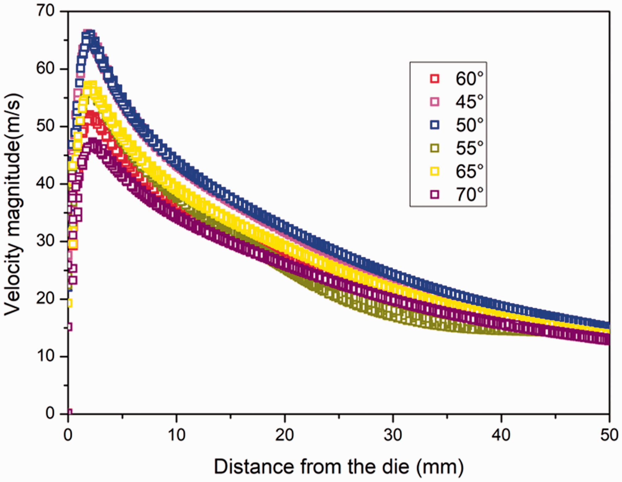
Figure 13 depicts the effect of slot angle on the polymer jet velocity with air flow rate of 40 slm. Six slot angles (45 $°$ , 50 $°$ , 55 $°$ , 60 $°$ , 65 $°$ , 70 $°$ ) were adopted in the comparison while the other dimensions of the die were consistent in the six cases. It was discovered that the polymer jet velocity isn’t simply increasing or decreasing with the increase or decrease of the slot angle. When the slot angle is 70 $°$ , the polymer jet has the lowest velocity. The polymer jet shows the highest velocity with the slot angle of 45 $°$ and 50 $°$ . It means that when the slot angle is 45 $°$ or 50 $°$ , the slot die has the best performance in attenuating the polymer jet.

Figure 13.

The effect of slot angle on the polymer jet velocity with air flow rate of 40 slm.

Conclusion

In the present work, to predict the motion of polymer jet during melt blowing, we have applied the phase field method to establish a model which included the coupling effect between air flow and polymer jet. We have made comparisons among the predicted value of the present model, the predicted value by the level-set method and the experimental value from our previous studies. The polymer jet velocity predicted by the present model is much higher than that predicted by the level-set method, and both of them are close to the experimental value in the area 20–50mm away from the die. The model built by phase-field method has showed superiority than that by level set method in predicting the final fiber diameter. Based on the model, the effect of polymer surface tension and slot angle on the polymer jet velocity were discussed.

Footnotes

Declaration of conflicting interests

The author(s) declared no potential conflicts of interest with respect to the research, authorship, and/or publication of this article.

Funding

The author(s) disclosed receipt of the following financial support for the research, authorship, and/or publication of this article: This work is funded by Funds for Key Disciplines of Nanhu (N41472001-43).

ORCID iD

Xibo Hao

References

Hao

Zeng

A review on the studies of air flow field and fiber formation process during melt blowing. Ind Eng Chem Res 2019; 58: 11624–11637.

Uyttendaele

MAJ

Shambaugh

RL.

Melt blowing: general equation development and experimental verification. AIChE J 1990; 36: 175–186.

Yin

Yan

Bresee

RR.

Experimental study of the meltblowing process. Int Nonwovens J 2002; 8: 60–65.

Shambaugh

RL.

Characterization of the melt blowing process with laser Doppler velocimetry. Ind Eng Chem Res 1992; 31: 379–389.

Yin

Yan

W-C

, et al. Fundamental description of the melt blowing process. Int Nonwovens J 2000; 9: 25–28.

Bresee

Qureshi

UA.

Influence of process conditions on melt blown web structure, part IV: fiber diameter. J Eng Fiber Fabr 2006; 1: 32–46.

Beard

Shambaugh

, et al. On-line measurement of fiber motion during melt blowing. Ind Eng Chem Res 2007; 46: 7340–7352.

Xie

Zeng

Online measurement of fiber whipping in the melt-blowing process. Ind Eng Chem Res 2013; 52: 2116–2122.

Rao

Shambaugh

RL.

Vibration and stability in the melt blowing process. Ind Eng Chem Res 1993; 32: 3100–3111.

10.

Marla

Shambaugh

RL.

Three-dimensional model of the melt-blowing process. Ind Eng Chem Res 2003; 42: 6993–7005.

11.

Chen

Huang

Modeling polymer air drawing in the melt blowing nonwoven process. Text Res J 2003; 73: 651–654.

12.

Zeng

Sun

Wang

XH.

Numerical approach to modeling fiber motion during melt blowing. J Appl Polym Sci 2011; 119: 2112–2123.

13.

Jarecki

Ziabicki

Mathematical modelling of the pneumatic melt spinning of isotactic polypropylene part II. Dynamic model of melt blowing. Fibres Text East Eur 2008; 16: 17–24.

14.

Sun

Yang

Sun

, et al. Simulation and modeling of microfibrous web formation in melt blowing. Ind Eng Chem Res 2016; 55: 5431–5437.

15.

Yin

Yan

Bresee

RR.

Experimental study of the meltblowing process. Int Nonwovens J 1999; 8: 1558925099OS-80.

16.

Hao

Huang

Zeng

Simulation of jet velocity in the melt-blowing process using the coupled air–polymer model. Text Res J 2018; 89.

17.

Harpham

Shambaugh

RL.

Flow field of practical dual rectangular jets. Ind Eng Chem Res 1996; 35: 3776–3781.

18.

Bansal

Shambaugh

RL.

On-line determination of diameter and temperature during melt blowing of polypropylene. Ind Eng Chem Res 1998; 37: 1799–1806.

19.

Marla

Shambaugh

Papavassiliou

DV.

Online measurement of fiber diameter and temperature in the melt-spinning and melt-blowing processes. Ind Eng Chem Res 2009; 48: 8736–8744.

20.

Bresee

W-C.

Fiber formation during melt blowing. Int Nonwovens J 2003; 12: 21–28.

21.

Comsol. CFD module user’s guide. 2015.

22.

Chhabra

Shambaugh

RL.

Experimental measurements of fiber threadline vibrations in the melt-blowing process. Ind Eng Chem Res 1996; 35: 4366–4374.

Simulation of polymer jet motion during melt blowing with phase field method

Abstract

Keywords

Introduction

Model construction

Geometry

Governing equations

Boundary conditions and mesh generation

Verification method

Results and discussion

Flow characteristics of polymer jet

Whipping motion of polymer jet

Verification of polymer jet velocity

Prediction of fiber diameter

Effect of surface tension on the polymer jet velocity

Effect of slot angle on the polymer jet velocity

Conclusion

Footnotes

Declaration of conflicting interests

Funding

ORCID iD

References