Automated measurements of fiber diameters in melt-blown nonwovens

Abstract

Fiber diameter and its distribution are the fundamental parameters affecting the performance of melt-blown nonwoven materials. This paper proposes a new method to measure diameters of microfiber in nonwoven based on image processing techniques. The one-pixel-wide boundaries of potential fibers were extracted first. The real fiber profiles were then separated from incorrect rectangles by a recognition procedure. Finally, the fiber diameters and diameter distribution were calculated. The experimental results show that the new method is consistent with the manual methods in measuring the main fiber diameter and fiber diameter distribution of melt-blown nonwoven material and has many advantages including efficiency, reproducibility, and objectivity.

Introduction

Microfibers refer to fibers whose linear density is in a range from 0.3 dtex to 1 dtex (1 dtex = number of grams/10,000 m) and have advantages in softness, specific area, and capillary wickability over other fibers [1]. As a result, products made from microfibers, such as melt-blown nonwovens, often posses excellent performance in filtration and conservation [2], highlighting the importance of the diameter of the microfiber.

In the melt-blown process, a thermoplastic polymer is extruded through a linear die containing several hundred small orifices, and streams of hot air rapidly attenuate the extruded polymer streams to form extremely fine filaments. These filaments are blown by high-velocity air onto a collector screen, thus forming a fine-filtered, self-bonded nonwoven web [3]. This web has multiple bonding points and the microfibers are tightly entangled, making the web difficult to dismantle for fiber diameter measurement.

Microfiber diameter measurement based on images from an optical microscope was the subject of the previous research. Wang et al. [4] analyzed the projection images of single fibers in a nonwoven web captured sequentially using a CCD camera. After noise removal and fiber profile extraction, the fiber obliquity was obtained through curve fitting, and then the diameter was determined with horizontal and vertical distances. They also conducted a preliminary study on fiber diameter distribution. Fan separated single fibers from a web image with edge enhancement procedures and then calculated the shaded area and stroke length-combining gray-level parameters extracted from the fiber width and orientation angle, thereby obtaining the shadow width [5]. Wang et al. introduced a method to capture microscopic images from thinned melt-blown nonwoven models and methods of image segmentation and skeleton extraction to calculate fiber diameters [6]. Yan and Bresee designed a procedure to segment fibers from non-fiber regions and determined fiber diameters with the horizontal or vertical fiber width and its orientation angle [7].

However, the above methods for measuring fiber diameters in nonwoven are suitable for thin samples where fibers are well focused and not overlapped except crossing points. Since scanning electron microscope (SEM) micrographs (see Figure 1) have a large depth of field, which is useful for understanding the surface structure of a sample [8], the current study proposes a method to measure microfiber diameter automatically based on SEM images. In this method, object boundaries are firstly extracted and parallel boundaries are connected into a series of rectangles representing potential fibers. Then, these rectangles are classified into real fiber profiles and false rectangles. Fiber diameters can be measured from the detected fiber profiles.

Figure 1.

Scanning electron microscope (SEM) images of melt-blown nonwovens.

Methods

In the current study, potential fiber profiles are constructed by pairing line segments (LS). Real fiber profiles and incorrect rectangles are then classified by a recognition procedure. The concrete steps of the proposed algorithm are as follows:

Detecting boundaries

Despite high sharpness and depth of field of the SEM images, there are pixels in the image where contrasts between targets (fibers) and the background are still not sufficient for perfect image segmentation when a simple thresholding is applied (see Figure 2). Therefore, a new algorithm to extract one-pixel-wide fiber boundaries was adopted in the current study. The new algorithm consists of three major steps. The Gaussian filter [9] was firstly used to remove image noise. The gradient operator [10] and iterative global thresholds [11] were then utilized to separate fiber boundaries from the background (Figure 3(a)). In the end, the thinning and pruning procedure was applied [12] to one-pixel-wide boundary extraction (Figure 3(b)).

Figure 2.

Thresholding segmentation of Figure 1(a).

Figure 3.

Boundary extraction (a) Edge detection and thresholding and (b) thinning and pruning.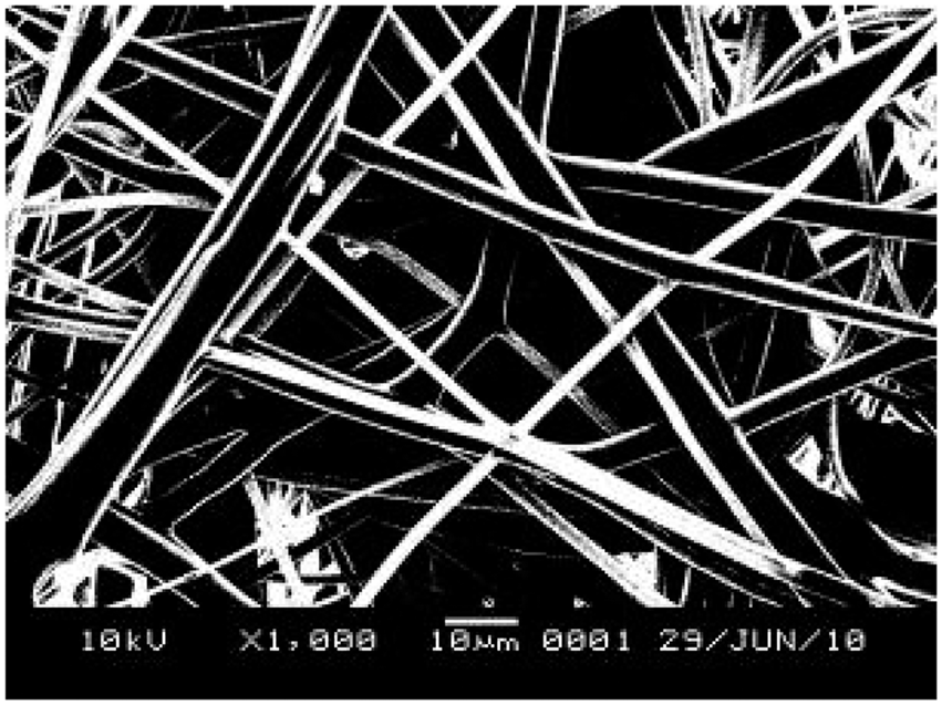

Amending boundaries

Figure 4(a) is a close-up view of a rectangular area in Figure 1(a), showing that fiber boundaries in a local region are almost straight and can be approximated by LS (Figure 4b). As a result, potential fiber profiles can be constructed by pairing LS. Flex points of the crossing boundaries should be deleted (point B) and the segments belonging to the same fiber boundaries should be connected, e.g., points E to F.

Figure 4.

Line segments (LS) of fiber boundaries (a) Enlarged view of a local region in Figure 1(a). (b) LS of fiber boundaries.

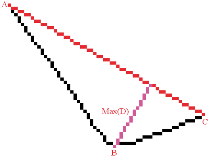
Figure 4(b) shows a fold line “ABC” extracted from two crossing fibers. The flex point “B” of the fold line can be deleted as follows:

Connect the endpoints A and C with a straight line (line AC in Figure 5);

Calculate the max perpendicular distance (Max(D)) from the black fold line to AC;

If Max(D)/LAC > T, delete point B. Here, LAC is the length of AC and T is a preset threshold. T was selected to be 3 in this project based on preliminary results.

Figure 5.

Schematic diagram of flex point deletion.

Segments DE and FG in Figure 4(b) belong to one fiber boundary, but are broken because of the interception with another fiber. To identify whether two broken segments are collinear, the slopes (k_DE and k_FG) of the segments and the distance (d_EF) between two near endpoints must satisfy the following conditions:

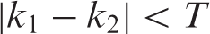
|k_DE – k_FG| < T₁, where T₁ is a threshold for checking the similarity of the slopes. The different LS on the same edge of fiber should have similar values of slopes. Considering computational accuracy, the threshold value in this paper is set as 0.1. If this is passed, then check

|k_EF – k_DE| < T₁ and |k_EF – k_FG| < T₁ (k_EF is the slope of EF). If this is passed, then check

d_EF  < T₂, where T₂ is set to check the distance of the slopes. The different LS on the same edge of the fibers will not be too far away. So the distance between two near endpoints should be smaller than a certain value. In this paper, this threshold value is set as 3 according our experiments.

After all the boundaries are amended, they are replaced by the straight lines (LS) that connect the endpoints of each boundary (see Figure 6).

Figure 6.

Line segments of fiber boundaries (a) and a close-up view (b).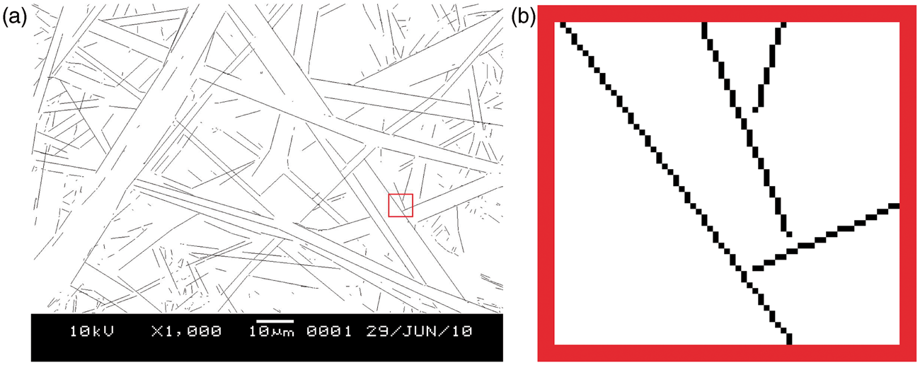

The LS of potential fiber profiles are paired based on their slopes:

$|k_1-k_2|<T$

(1)

where, k₁, k₂ are the slopes of two LS; T is 0.05. Then rectangles were drawn using the paired LS as long sides. Figure 7 displays the potential fiber profiles in the whole SEM image.

Figure 7.

Fiber profiles (a) and enlarged view (b).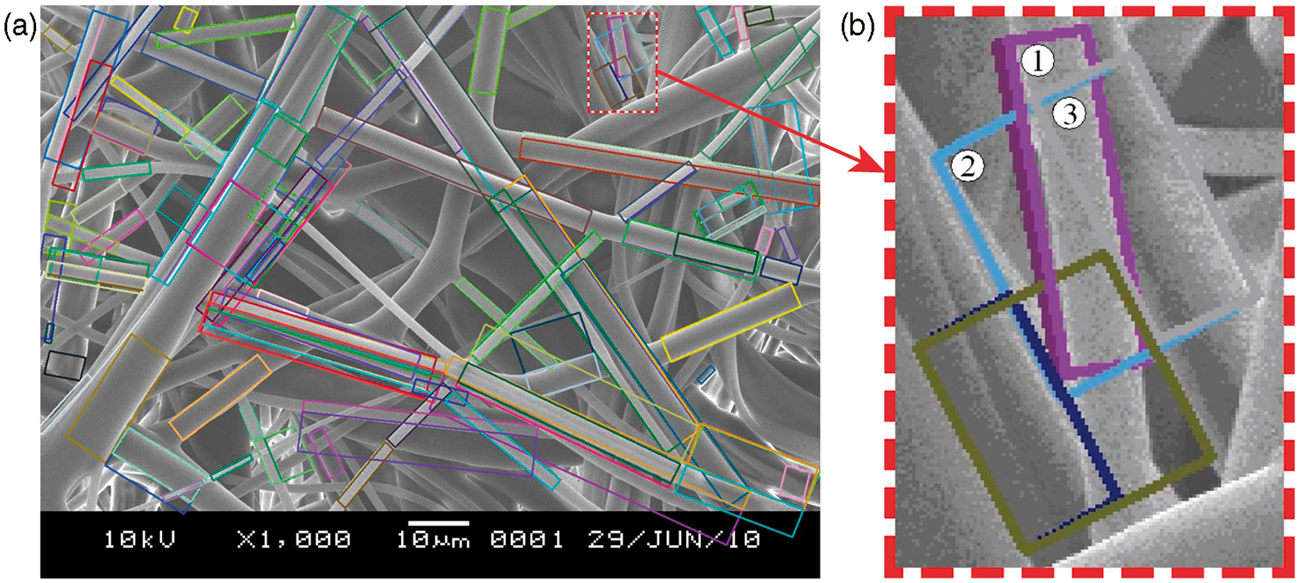

Removing incorrect rectangles

Of the paired LS, there may be LS that belong to different fibers as seen in Figure 7(b) (rectangles 2 and 3). Rectangle 2 is incorrect because it contains two touching fibers. In the SEM image, the fiber structure demonstrate a trend that its grayscale moves from light to dark and then back to light across the fiber width. This feature can be revealed by a grayscale histogram, and used to separate fiber profiles from incorrect rectangles.

Figure 8 shows rectangle “ABCD” that is a potential fiber profile. In the rectangle, lines AB and CD are the fiber boundaries and lines AD and BC are edges perpendicular to the fiber boundaries. The intensity (gray value) changes across the fiber boundaries can be found as follows:

Locate each pixel on AD and BC;

Starting from a pixel on AD (e.g., E), locate the pixels on a line that is parallel to AB and ends at F on BC;

Add the gray values of all the pixels on EF in the SEM image;

For each pixel on AD, a perpendicular line can be determined and the sum of gray values of the line pixels can be obtained. After the normalization, the traverse intensity curve can be drawn (see Figure 9).

Figure 8.

Line-segment rectangle.

Figure 9.

Intensity curves of rectangles in Figure 7(b); (a) Rectangle 1; (b) Rectangle 2; and (c) Rectangle 3.

Figure 9 shows three different intensity curves of the rectangles. The curve of a correct fiber profile should have only one downward wave (Figure 9(a) and (c)), the curve of an incorrect rectangle often has two or more waves (Figure 9(b)). Therefore, two characteristic parameters F₁ and F₂ are defined for classifying correct fiber profiles and incorrect rectangles:

$F_1=N_v,F_2=\frac{A_s}{W}$

(2)

where N_v is the number of wave valley; A_s is area of the shaded portion; and W is the number of pixels along the rectangle width.

F₁ and F₂ of the rectangles in the image can be organized in a two-dimensional parameter space, and a probability density distribution map can therefore be drawn by calculating the probability of point locations of rectangles in the parameter space [13], as shown in Figure 10 where there are eight grade probability contours, i.e., 12.5% probability per grade.

Figure 10.

The probability density distribution map of F₁ and F₂.

Figure 10 shows that the real fiber profiles have fewer wave valleys (F₁) and larger shaded area ratios (F₂). Inversely, incorrect rectangles have higher F₁ and lower F₂. Hence, these two classes can be separated by establishing a decision boundary in the F₁ – F₂ map. In the overlapping region of real fiber profiles and incorrect rectangles, the decision boundary is the curve that makes the minimum probability of classification mistake. To ensure the accuracy of the diameter testing, the decision boundary has been set towards the real fiber profiles (see the separation curve in Figure 10). Take Figure 7(a) as an example. There were 134 rectangles in the image, of which 58 were classified as real fiber profiles and 76 incorrect rectangles (Table 1). The Accuracy rate for classifying real fiber profiles is almost 95%. Figure 11 displays the real fiber profiles determined by the classification algorithm.

Figure 11.

Real fiber profiles.

Table 1.

Classification result of rectangles.

Real fiber profiles	Incorrect rectangles
Classified	58	76
Manually counted	55	69
Accuracy rate (%)	94.83	90.79

Merging fiber profiles

The fiber profiles are then merged to avoid repeated testing. The widths of profiles are firstly calculated by the following equation:

$W=\frac{|C_2-C_1|}{\sqrt{A^2+B^2}}$

(3)

where W is the width of a profile. Ax + By + C₁ = 0 and Ax + By + C₂ = 0 are equations of the long boundaries of the profile.

The merging of the profiles, which belong to the same fiber, is based on the following conditions:

$|W_1-W_2|<T_3|{\theta }_1-{\theta }_2|<T_4|{\theta }_M-{\theta }_1|<T_4$

(4)

where

W₁, W₂ are the widths of two profiles;

T₃ is a threshold (=5) taking the local difference in fiber width into consideration;

θ₁, θ₂ are orientation angles of two profiles;

θ_M is the orientation angle of the merged profile.

T₄ is an angle threshold that is set to 0.05, considering computational accuracy.

This step repeats until no profiles need to be merged. Figure 12 exhibits the fiber detection results of Figure 1 after the merging process.

Figure 12.

Fiber detection results of Figure 1.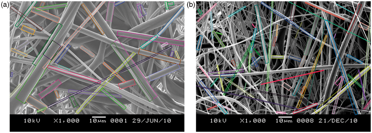

Calculating fiber diameter distributions

The fiber diameter of a detected fiber profile is equal to the width of the rectangle. After all the detected fibers in the image are counted, the diameter distribution curve can be drawn from the frequency counts. The main diameter is obtained through the ridge position of the curve.

Experiment and discussion

Eight different melt-blown materials (Table 2) were selected as the samples in the experiment. The SEM used in our experiment is COXEM CX-100 S with resolution of 6.0 nm. For each sample, more than 20 SEM images with 1000 magnification were captured at different positions. More than 1500 fibers were tested by both the proposed method and the traditional manual method.

Table 2.

Material used as samples.

1#	2#	3#	4#	5#	6#	7#	8#
Fiber type	Polypropylene  (PP)	PP	Polyester  (PET)	PP	PP	PP	PET	PP
Areal density (g/m2)	20.23	14.98	24.2	38.17	32.49	10.51	25.16	18.81
Thickness (mm)	0.271	0.121	0.181	0.359	0.224	0.087	0.187	0.136
Porosity	75.2%	83.6%	80.3%	73.1%	71.7%	89.2%	73.5%	78.9%

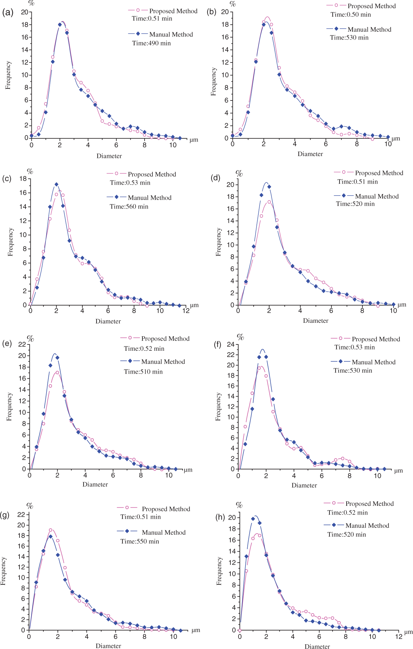
The experimental results show that diameter distribution curves obtained from the proposed method are in good agreements with the curves obtained from the manual method (Table 3), as seen in Figure 13(a–h). However, the manual method needed approximately 500 min to finish the fiber measurements in 20 images (25 min/image), while the proposed method required only around 0.5 min (1.5 s/image). Therefore, the proposed method greatly improves the efficiency of measuring fiber diameter distributions in an SEM image while maintaining the same level of accuracy as the manual method.

In average, the manual method costs about 20–30 min to test a single SEM image, while the proposed method only needs 1.5 sec. If this efficient method is applied, it will be able to provide a more rapid diameter test for melt-blown nonwoven materials.

Fibers with larger diameter are often covered by other fibers; they are easy to be missed. As a result, the accuracy of the diameter distribution curve will decrease. As these fibers occur in small numbers, they have very little effect to the main diameter of melt-blown nonwoven materials.

In our experiments, we use different melt-blown nonwoven with different areal density, thickness, and porosity as samples. Because of the large depth of field of SEM micrographs, the diameter tested by the proposed method is in good agreement with manual method. The proposed method is suited for diameter measurement of melt-blown nonwovens.

There are several thresholds in the algorithm: the threshold T in the procedure removing the flex points, the T₁ and T₂ during connecting boundaries, and another T₃ and T₄ in merging fiber profiles, among others. These thresholds will influence the accuracy of the proposed algorithm. Their values in this paper are best cited by our experiments.

Table 3.

R² of the proposed and manual methods.

1#	2#	3#	4#	5#	6#	7#	8#
R2 (%)	99.31	98.92	99.27	99.01	99.43	98.84	99.03	98.72

Figure 13.

Diameter distribution curves of eight different melt-blown nonwovens.

Conclusions

Fiber diameter distributions have direct impacts on the performance of melt-blown nonwoven materials, especially on filtration and barrier efficiency. The current study proposes a new image-analysis method for measuring the microfiber diameter of melt-blown nonwoven materials automatically. The experiment with eight different melt-blown nonwovens prove that the main fiber diameters and fiber diameter distributions derived from the proposed method are in high agreements with those derived from the manual method; but the proposed method is almost 1000 times faster than the manual method.