Sage Journals: Discover world-class research

Abstract

Although economists regularly use sports to study labor-market outcomes, nearly all sports-related studies focus on men. Instead, this paper looks at career breaks and career exits for women's basketball, with a focus on race/ethnicity and country of birth. Data are from the start of the Women's National Basketball Association in 1997 through the 2019 season. White players and foreign-born players have higher likelihoods of leaving the league, conditional on player demographics and productivity.

Keywords

employment race/ethnicity immigration basketball

Introduction

In many areas of economics, sports provide a great opportunity to study economic concepts. Labor economists are particularly fond of sports because data on productivity are more readily available than in nonsports jobs. Gender-based gaps in employment and pay are narrowing in sports, with soccer and tennis leading the way in terms of equal pay.

At the same time, Brittney Griner's Russian arrest in February 2022 highlights disparities between male and female basketball players. For example, in 2019, the salary cap was $996,100 per team in the Women's National Basketball Association (WNBA) and almost $102 million per team for the (men's) National Basketball Association (NBA). With such vast differences, the determinants of employment and salaries likely differ between men and women. Yet, the overwhelming majority of research in sports economics focuses on men's sports.

This paper provides new evidence on the determinants of employment breaks for women in professional sports, using data from the inception of the WNBA in 1997 through the 2019 season, the last season before the onset of the global pandemic. Specifically, I use a semiparametric hazard model to study career exit, along with a simple logit model to study career breaks. Salaries are not a dependent variable because salary data are only available from 2018.

Of particular interest are the roles of race/ethnicity and country of birth, given the considerable research on these two attributes in men's basketball. No clear consensus has emerged on the relationship between employment and race in the NBA, whereas international players generally have shorter careers (Groothuis & Hill, 2004, 2013, 2018). I am unaware of any previous work on determinants of employment in any women's sports.

In the WNBA, White players are approximately four percentage points more likely to exit, either temporarily or permanently. Compared with U.S.-born players, international players are also more likely to exit, particularly for players that did not play U.S. college basketball. More productive players, and players drafted in the first round, are less likely to leave. This pattern of results is robust to different ways of modeling productivity or experience. Results are qualitatively similar for the full sample of players as well as the select sample of starters.

Relationship to Literature

The economics literature on women's basketball is quite small. Only two papers look at individual players. Harris and Berri (2016) study the determinants of playing time in the WNBA, focusing on player and coach race. In a model with team fixed effects, they find no differences in playing time by race aside from a marginally significant, negative association of lower playing time for players with non-White coaches. Brown and Jewell (2006) estimate the marginal revenue product of women's college basketball players at approximately $250,000.

Most of the women's basketball literature focuses on teams rather than players, often looking at differences by gender. The literature documents gender differences across a variety of topics including the pay of college basketball coaches (Humphreys, 2000), the willingness to pay for college basketball tickets (Rosas & Orazem, 2014), the predictability of college basketball players’ behavior (Gokcekus et al., 2010), and differences in efficiencies and playing style (McGoldrick & Voeks, 2005). In contrast, authors find no differences by gender in the likelihood of “tanking” in professional basketball (Hill, 2021), late-game free-throw percentages (Toma, 2017), determinants of collegiate basketball attendance (Depken et al., 2011), betting strategies on professional basketball (Paul & Weinbach, 2014), and team draft strategies (Harris & Berri, 2015).

The literature on men's basketball, primarily on the NBA, is extensive. Several papers look at the determinants of employment and salary, and most of these papers focus on race. The consensus in the literature is that, at least among studies with multiple time periods and extensive controls, the relationship between race and salaries has varied over time. Research covering the late 1980s through the 2000s found few if any racial differences in salaries (Dey, 1997; Groothuis & Hill, 2013; Hill, 2004; Naito & Takagi, 2017; Robst et al., 2011). Starting in the 2010s, researchers have found higher salaries for White players (Johnson & Minuci, 2020; Naito & Takagi, 2017). Looking at single years, Kahn and Sherer (1988) and Kahn and Shah (2005) find a salary premium for White players, whereas Ajilore (2014) and Gius and Johnson (1998) report no racial differences in salaries. Looking at career length rather than salaries, the results are also mixed. Hoang and Rascher (1999) document shorter careers for Black players, whereas Groothuis and Hill (2004, 2013) find no racial difference in career length once they control for player height.

The NBA literature also looks at employment and salary differentials between U.S.-born and foreign-born players. Eschker et al. (2004) and Hill and Groothuis (2017) find higher salaries for foreign-born players only for seasons before 2000 when the share of such players was quite small.¹ In contrast, Yang and Lin (2012) document lower salaries for foreign-born players in the early 2000s from a two-stage model. Hill and Groothuis (2017) note that, among players who play U.S. college basketball, foreign-born players have similar salaries to U.S.-born players. Groothuis and Hill (2004, 2013) report that foreign-born players and U.S.-born players have similar career lengths, whereas Groothuis and Hill (2018) show that international players who did not play college basketball in the U.S. have shorter careers than U.S.-born players. Thus, I contribute to the sports economics literature by examining the role of race and country of birth on employment breaks in the WNBA.

Data and Descriptive Statistics

The data come from the Basketball Reference website (www.basketball-reference.com/wnba/). Data cover the first season of the WNBA in 1997 through the last pre-pandemic season of 2019, although data from 2019 are used only to measure employment (as explained further in the next section). The panel database contains 3,573 player seasons across 923 players and 22 seasons. Demographic data include height, country of birth, experience, and race/ethnicity.² Player race and ethnicity are determined by viewing player photographs available online from a combination of the Wikipedia, WNBA, and Basketball Reference websites. Harris and Berri (2016) also use this approach, given the lack of published data on WNBA player race/ethnicity. One concern with collecting my own data is the possibility of data entry errors. To improve the accuracy of the race and ethnicity data, two individuals (the author and a research assistant) looked at each player’s photograph. Computer-based analysis, such as the study on skin tone in the NBA (Robst et al., 2011), is a potential data source for future work.

I use three measures of player performance from the Basketball Reference website. The first measure is win share, an adaptation of the baseball statistic of the same name devised by Bill James.³ In essence, the formula divides each win among the players on the team using information on several statistics such as points scored and possessions. In other words, if a team won a single game using 10 players who contributed equally, the win share would be 0.1 for each player. An alternate metric is wins produced, first introduced in Berri (1999), which incorporates shooting efficiency.⁴ Due to limited data availability for wins produced, along with the high correlation between wins produced and win share (0.87), I do not use wins produced.

The second measure of performance divides win share into separate variables for offense and defense. The third and final measure of performance⁵ is the player efficiency rating, a measure of the per-minute productivity of each player. Win share (the first measure) is the preferred one due to its simplicity and ease of interpretation.

The outcome of interest is a break in employment. WNBA players have substantial mobility from season to season. Salary data are not used as outcomes because salary data for the WNBA are publicly available starting in 2018, and most salaries are entry-level contracts determined by collective bargaining agreements (CBAs) rather than by WNBA performance, race/ethnicity, or country of birth.

Table 1 contains the descriptive statistics for the panel database. The unit of analysis in the top panel is a player in a season, with 3,573 observations. In other words, an observation is a given player in a given season. The bottom panel presents player-level data on time-invariant characteristics for the 923 players in the data. The two employment measures illustrate the high level of player turnover in the WNBA. In a given season, 28.2% of players do not return for the following season, and 22.6% of players leave the league without ever returning (during the time period).

Appendix Table 1.

Interactions With Collective Bargaining Agreements (CBAs).

	Career Exit			Career Break
	Marginal	Standard		Marginal	Standard
	Effect	Error		Effect	Error
1999 CBA
White	0.057	0.024	**	0.054	0.026	**
International, no college	0.002	0.029		0.077	0.036	**
International, college	0.037	0.048		0.079	0.042	*
2003 CBA
White	0.006	0.029		−0.006	0.032
International, no college	0.120	0.059	**	0.260	0.067	***
International, college	0.021	0.047		0.091	0.051	*
2008 CBA
White	0.037	0.028		0.039	0.032
International, no college	−0.024	0.044		0.072	0.060
International, college	0.098	0.042	**	0.134	0.059	**
2014 CBA
White	0.055	0.037		0.049	0.041
International, no college	0.081	0.049	*	0.115	0.052	**
International, college	−0.003	0.047		−0.055	0.048
Chi-squared test statistic for equality among 4 CBAs
	Stat.	Prob>0		Stat.	Prob>0
White	2.04	0.564		2.35	0.503
International, no college	6.32	0.097		6.84	0.077
International, college	3.64	0.303		10.24	0.017
Pseudo R-squared	0.322			0.286

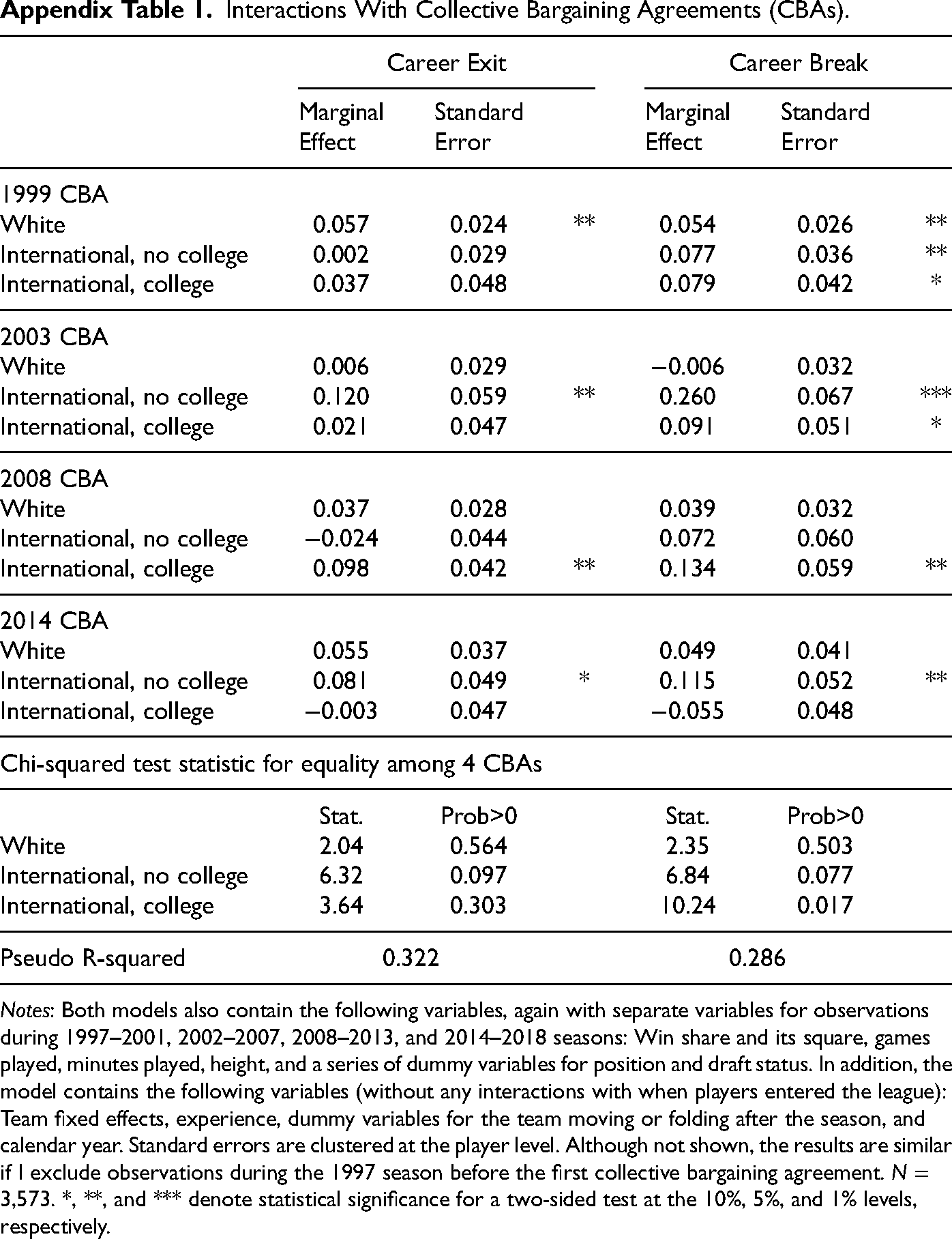
Notes: Both models also contain the following variables, again with separate variables for observations during 1997–2001, 2002–2007, 2008–2013, and 2014–2018 seasons: Win share and its square, games played, minutes played, height, and a series of dummy variables for position and draft status. In addition, the model contains the following variables (without any interactions with when players entered the league): Team fixed effects, experience, dummy variables for the team moving or folding after the season, and calendar year. Standard errors are clustered at the player level. Although not shown, the results are similar if I exclude observations during the 1997 season before the first collective bargaining agreement. N = 3,573. *, **, and *** denote statistical significance for a two-sided test at the 10%, 5%, and 1% levels, respectively.

Turning to productivity, the mean for win share is 1.33, implying that the average player is solely responsible for more than one win per season. The most productive player is responsible for 10 wins, whereas the least productive player is responsible for nearly 2 losses. The offensive and defensive win shares are roughly equal at the mean, but the offensive win share has more outliers at both ends of the distribution. Finally, the personal efficiency rating has a mean of 12, although the scale ranges from −112 to 79. The share of players with negative productivity varies from measure to measure, ranging from approximately 5% for defensive win share and player efficiency rating to more than 20% for offensive win share.

On average, players participate in 25.6 regular season games per year (out of 34 in most seasons) and over 500 minutes per year (out of 1360 minutes in most seasons).⁶ The average experience is approximately three seasons. In 2% of observations does a player experience a team changing location or folding after the current season.

Turning to player-level variables, approximately one-third of the players are White, and two-thirds are Black. Under 3% are Asian, Hispanic, or Native American. Nine percent of players were born outside the U.S. but attended college in the U.S., whereas 14% were born outside the U.S. and did not play U.S. college basketball. The average height is six feet tall, or 72 inches. Nearly half the players are guards and over 40% are forwards.⁷ Thirty percent are first-round draft picks, and 23% are second-round draft picks.

Methods

Breaks in employment, the outcomes of interest, are modeled in two ways. The first is a semi-parametric hazard model of career length. This model is used in Groothuis and Hill (2004, 2013, 2018) for the NBA, Berger and Black (1998) for Medicaid spells, and Berger et al. (2004) for health-insurance-related job mobility. This model incorporates both the “stock” of WNBA players in a given season but also the “flow” of players throughout their careers, using the terminology of Lancaster (1990).

Because the model has been discussed thoroughly in previous work, I provide an overview here. Define $f (t, x, β)$ as a density function⁸ of player characteristics x (discussed further in equation (2)), t as the length of the spell, and $β$ as a vector of coefficients. The characteristics are the demographic and performance indicators listed in Table 1, as well as dummy variables for position, calendar year, and team. The associated cumulative distribution function is $F (T, x, β) = \Pr (t \leq T | x)$ . Then, the survivor function, the likelihood of being in the WNBA in season T, is $S (T, x, β) = (1 - F (T, x, β))$ .

One advantage of the data set is the availability of WNBA data since its inception. Thus, left censoring—players who were already in the league at the start of the analysis period—is not a concern. The only censoring is the right-hand censoring of players who are still employed in the WNBA at the end of the sample period in 2019. Therefore, the likelihood function used in Berger and Black (1998) and subsequent research simplifies to

L (β) = \prod_{i \in A} f (t_{i}, x_{i}, β) * \prod_{i \in B} S (t_{i}, x_{i}, β)

(1)

As defined above, f is the density function and S is the survivor function. Set A contains the set of players who are not right-hand censored (i.e., who finish playing in the WNBA before the 2019 season), whereas set B contains players who are right-hand censored, as they are still in the league in 2019.

I estimate the following hazard model, as in Groothuis and Hill (2004):

\frac{h (t, x, β)}{[1 - h (t, x, β)]} = Θ (t) e^{x β} = \exp (ϕ [t] + x β)

(2)

In this equation, h is the hazard function;

Θ

and

ϕ

denote functions of tenure in the league. Berger and Black (1988) use an exhaustive set of dummy variables for each year of tenure. Given the short career lengths of most NBA players, Groothuis and Hill (2004, 2013) use a fourth-order polynomial of tenure; Groothuis and Hill (2018) use a fifth-order polynomial. I estimate polynomial models and dummy variables models to test the sensitivity of the results to the way in which tenure is parameterized. The preferred model uses dummy variables for each year of experience up to 13 years. Because only 6 observations have more than 14 years of experience—4 with 15 years and 2 with 16 years—a single dummy variable denotes 14 or more years of experience.

As in most previous work, I estimate a logit function. The hazard function on the right-hand side is depicted as a dummy variable equal to 1 for a player's last season in the league and zero for all other seasons. For players still in the league in 2019, the dummy variable is equal to zero in all seasons. I also explore the use of a probit model as specified in Groothuis and Hill (2013). I do not estimate a linear probability model because, as noted in Groothuis and Hill (2004), the hazard function must have a range from zero to one. In linear probability models, the estimated probability can lie outside this range, and this situation occurs in the linear probability models for the WNBA.

Two underlying assumptions of the model are worth noting in this application to sports. First, the only way in which the calendar year affects the model is through the dummy variables for the calendar year included in the logit model. Otherwise, the determinants of player exit are assumed to be the same across calendar years. In other words, the likelihood of a third-year (or any other year) player continuing in the league is the same whether that player's third year is in 1999 or 2009.⁹ The second assumption is to ignore career breaks. A nontrivial number of players in the WNBA miss a season (or more) due to reasons such as injury or childbirth. To keep the model as simple as possible, such breaks are ignored in the career exit model.

Given the challenges of defining “exit” from the league when players return after multiple years away, the second model is a simple logit model estimating career break as a function of player characteristics and the previous season's productivity, shown in equation (3):

Prob (Y_{i t + 1} = 1) = F (α + X_{i t} * β + TEA M_{j} + δ_{t})

(3)

In this equation, Y is a dichotomous variable equal to 1 for players who did not play in the WNBA in season t+1 and 0 for those did. This outcome—denoted as a career break—does not distinguish between temporary and permanent exits; in both cases, the dependent variable equal to 1. As in the hazard model, an observation is a player in a season, such as Cynthia Cooper in the inaugural 1997 season, where she was the most valuable player. The seasons for t are from 1997 to 2018, so that employment in season t+1, 1998–2019, occurs prior to the pandemic. F is the cumulative logistic distribution, although the results are robust to the use of a probit model.

The set of player characteristics X consists of two components, demographics and performance. The main demographic variables of interest are race and foreign-born, given the extensive literature on these demographics in the NBA. For race, a dummy variable is equal to one for White players. The omitted group is non-White players, nearly all of whom are Black.¹⁰ For foreign-born, I follow Groothuis and Hill (2018) and estimate two separate foreign-born variables, one for those who played college basketball in the U.S. and another for those who did not. All the U.S.-born players in the data set played college basketball in the U.S. The equation also includes additional demographics for experience (measured as a set of dummy variables, as in the preferred hazard model specification), height, position, and draft round, as shown in Table 1. Finally, the equation includes calendar year fixed effects.

As discussed in the previous section, the data contain multiple measures of performance. For simplicity, win share, its square, games played, and minutes played are the preferred measures of performance. Again, robustness tests are conducted to test the sensitivity of the results to the choice of performance measures. The equation also includes team-fixed effects to account for all time-invariant differences across teams. Teams that move are still considered the same team, such as the Orlando Wizards moving to Connecticut as the Connecticut Sun. Finally, standard errors are clustered at the player level. Note that the set of characteristics is the same for both outcomes to facilitate comparison between models.

Results

Main Results

Table 2 contains the logit model results for the two measures of employment. The left panel is for career exit (as in previous work), and the right outcome is for a career break. For ease of interpretation, the tables contain marginal effects and their standard errors (clustered at the player level). Recall that the outcome is equal to one for a player who leaves the league, either permanently or temporarily, so positive marginal effects indicate a positive association with leaving.

Appendix Table 2.

Determinants of Career Exits and Breaks Alternate Definition of International Players.

	Career Exit			Career Break
	Marginal	Standard		Marginal	Standard
	Effect	Error		Effect	Error
White	0.044	0.014	***	0.044	0.017	***
International	0.035	0.017	**	0.092	0.022	***
Win share	−0.067	0.010	***	−0.051	0.011	***
Games played	−0.004	0.001	***	−0.005	0.001	***
Minutes played (00s)	−0.036	0.005	***	−0.036	0.005	***
Height (inches)	−0.007	0.003	***	−0.004	0.003
Center	0.027	0.020		0.018	0.024
Forward	0.025	0.014	*	0.014	0.017
Drafted first round	−0.080	0.014	***	−0.079	0.017	***
Drafted second round	−0.033	0.014	**	−0.020	0.017
Team moved after season	0.054	0.045		0.059	0.049
Team folded after season	0.002	0.043		0.012	0.051
Pseudo R-squared	0.324			0.285
Mean dependent variable	0.226			0.282

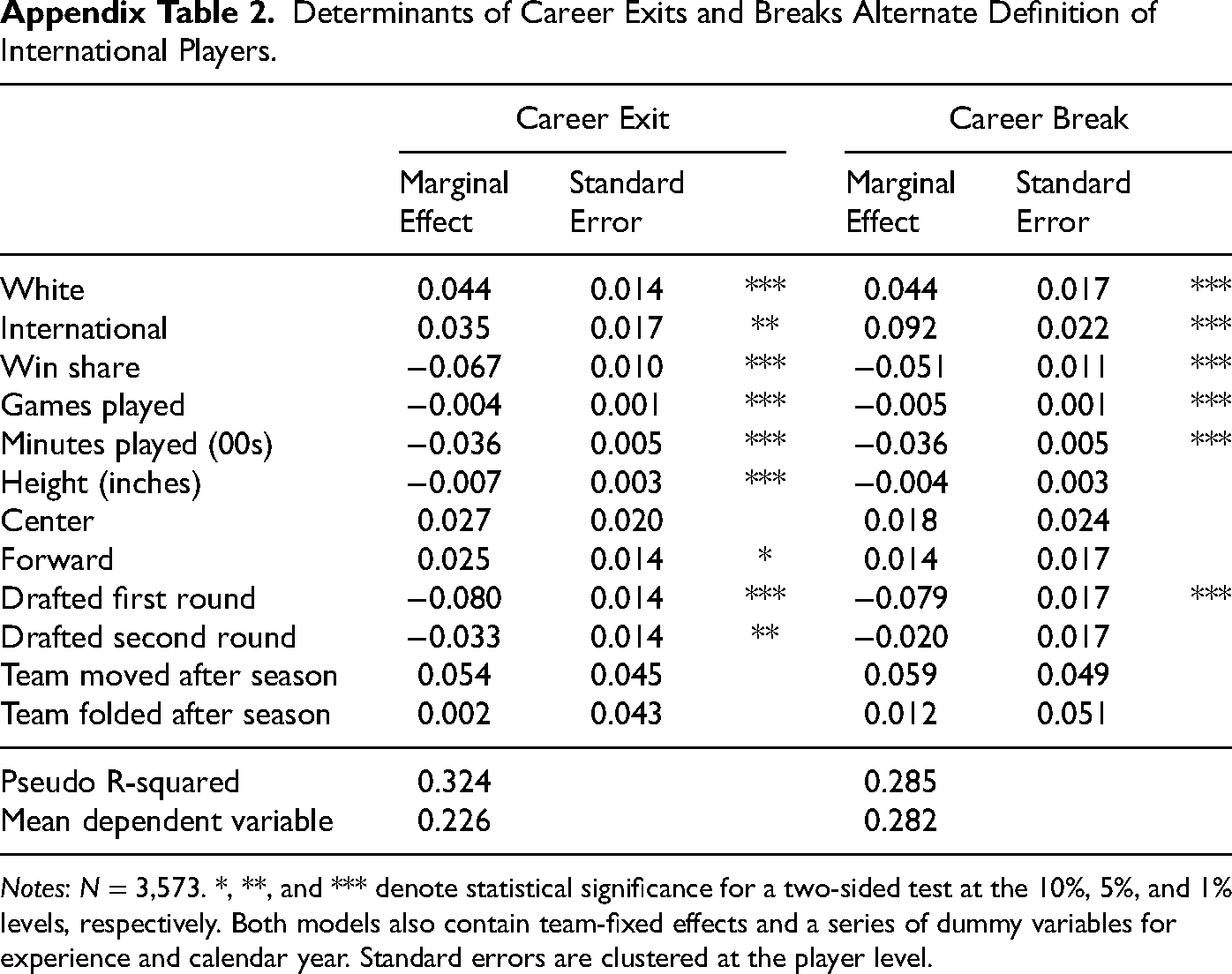
Notes: N = 3,573. *, **, and *** denote statistical significance for a two-sided test at the 10%, 5%, and 1% levels, respectively. Both models also contain team-fixed effects and a series of dummy variables for experience and calendar year. Standard errors are clustered at the player level.

The marginal effects for international players are more pronounced for career breaks. This result is not surprising as career exits (mean = 0.226) are a subset of career breaks (mean = 0.282). White players are approximately four percentage points more likely to leave the league, either permanently or for a career break of one season or more. This result contrasts with the literature in the NBA, where race is generally uncorrelated with employment (Groothuis & Hill, 2004, 2013, 2018).

International players with no U.S. college experience have a marginally higher likelihood of career exit of 0.042, whereas they have a 12 percentage-point higher likelihood of taking a career break. For example, some international players skip the WNBA season in Olympic years given that both take place in the summer. International players with college experience have a marginally higher likelihood of a career break of 0.053, but the coefficient for career exit is only 0.025 and is not statistically significantly different from zero at the 10% level (for a two-sided test). For comparison with the NBA, Groothuis and Hill (2018) report higher rates of career exit for international players with no U.S. college experience, but they find similar rates of career exit between U.S.-born players and international players who played U.S. college basketball.

Productivity is negatively correlated with both outcomes. Because win share is modeled with both linear and quadratic effects, Figure 1 illustrates its marginal across the distribution, from the first percentile to the 99th. For nearly all of its distribution, win share has a negative effect, with more pronounced negative effects for the players with the least productivity. For career exit, win share's marginal effect for a player at the 10th percentile is −9.3 percentage points, compared with −6.4 percentage points at the median and −0.9 percentage points at the 90th percentile.

Figure 1.

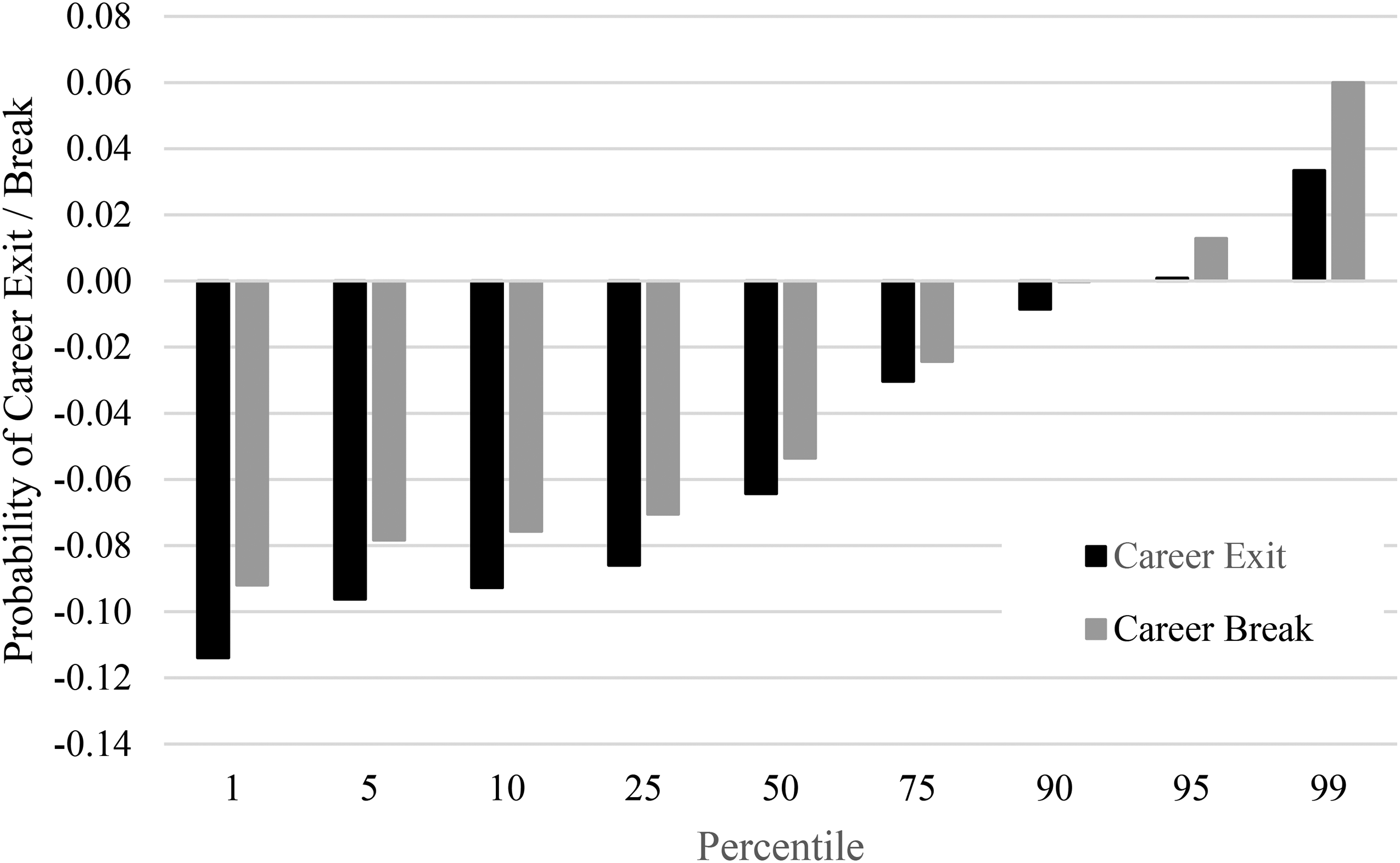
Marginal Effect of Win Share on Career Exits and Career Breaks.

Each game played is associated with a 0.4 percentage-point decrease in career exit, whereas an increase in minutes played of 100 minutes is correlated with a 3.6 percentage-point decrease in career exit. For a career break, the percentage-point decreases are 0.5 for games and 3.6 for minutes played.

Player characteristics are often significant determinants of career exits and career breaks. Taller players are more likely to exit the league, although the effects are modest in magnitude. An additional inch of height corresponds with a 0.7 percentage-point decrease in the likelihood of a career exit. The height coefficient for a career break is only −0.3 percentage points, and I cannot reject the hypothesis that there is no correlation between height and career break at the 10% level for a two-sided test. Controlling for height, position has little relationship with employment. First-round draft picks are much less likely to exit the league, with marginal effects of −0.079 for career exit and −0.074 for career break.

Collective Bargaining

The relationship between employment and race/ethnicity and country of birth varies by time period in the NBA. To explore whether the same is true in the WNBA, I divide the data into four periods, each of which covers a separate CBA: 1997–2002, 2003–2007, 2008–2013, and 2014–2018. Recall that employment is measured in the following season, such as in 2003 for observations from the 2002 season. Each CBA came into effect in the first half of the year, before the WNBA season. For example, the 2003 CBA occurred in April. Thus, the relevant CBA for observations during the 2002 season is the 2003 agreement because the 2003 employment, which determines a career exit or career break, is during the 2003 CBA. The 1997 observations are included in the 1999 CBA despite not being covered by it to avoid left censoring in the hazard model (as in Groothuis and Hill, 2013) that would occur if these observations were excluded. Results are similar if the 1997 observations are excluded.

To compare the results across time periods, I estimate a single logit model with four sets of variables, corresponding to the control variables in each of the four time periods above. In other words, instead of having one variable for games played, I now include four variables for games played: one equal to the games played in that season for the 1997–2002 seasons (and zero for observations in other seasons), and the corresponding games played variables for observations in either 2003–2007, 2008–2014, or 2010–2018. The results are in Appendix Table 1.

For career exit, although the results vary by CBA, I can never reject the hypothesis (at the 5% level for a two-sided test) that the coefficients for each demographic such as race are equal across time periods. The marginal effects are often sizable and imprecisely estimated.

For career break, by far the largest marginal effect is 0.26 (more likely to take a career break) among international players with no U.S. college basketball experience, measured during the 2003 CBA. For the other 3 CBAs, the marginal effect is economically significant at 0.07–0.12 despite being statistically insignificant in the 2008 CBA. International players with college experience have a 13.4 percentage-point higher probability of a career break during the 2008 CBA, but the marginal effect is negative and statistically insignificant in the 2014 CBA. The marginal effect for White players is significant at 0.054 in the 1999 CBA; it is not nearly as large—and is less precisely estimated—in the 2008 and 2014 CBAs.

Although, presumably, the players gained more bargaining power and better working conditions with each successive CBA, the marginal effects show no discernable pattern over time. However, with a small sample of players in each season, standard errors and confidence intervals are large, severely limiting the ability to detect any potential effects of CBAs.

Sensitivity Analysis

In the NBA, researchers often do not distinguish between college attendance and not for international players. For comparison with those studies (such as Groothuis & Hill, 2013), Appendix Table 2 includes a single “international” variable. Another reason for estimating this model is that, in Table 2, I cannot reject (at the 5% level) the hypothesis that the two international variables have equal marginal effects. International players are more likely to have a career exit of 3.5 percentage points, and they are more likely to have a career break of 9.2 percentage points. Thus, international players have considerably more churn than domestic players, although the evidence of differences in career exit is less pronounced for international players.

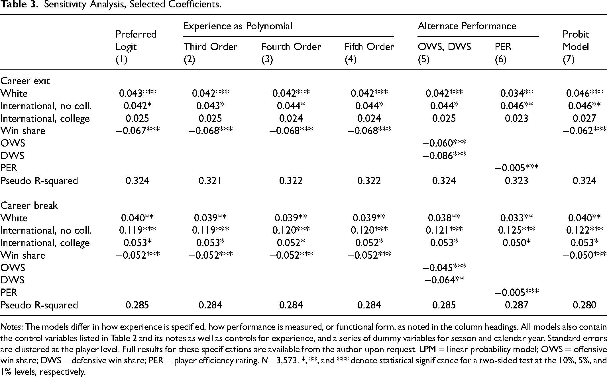
The next sensitivity analysis is for experience. In the preferred model from Table 2, experience is measured by a series of dummy variables as done in the original applications of the model in Berger and Black (1998) and Berger et al. (2004). I estimate three additional specifications, where experience is a polynomial of third-order, fourth-order (as in Groothuis & Hill, 2004, 2013), or fifth-order (as in Groothuis & Hill, 2018). The results for these models, and additional sensitivity analyses, are in Table 3. The first column is the preferred model; columns 2–4 are for different polynomials in experience; columns 5 and 6 have alternate measures of performance, and the final column is from a probit. The top panel is for career exit, and the bottom panel is for career break.

Appendix Table 3.

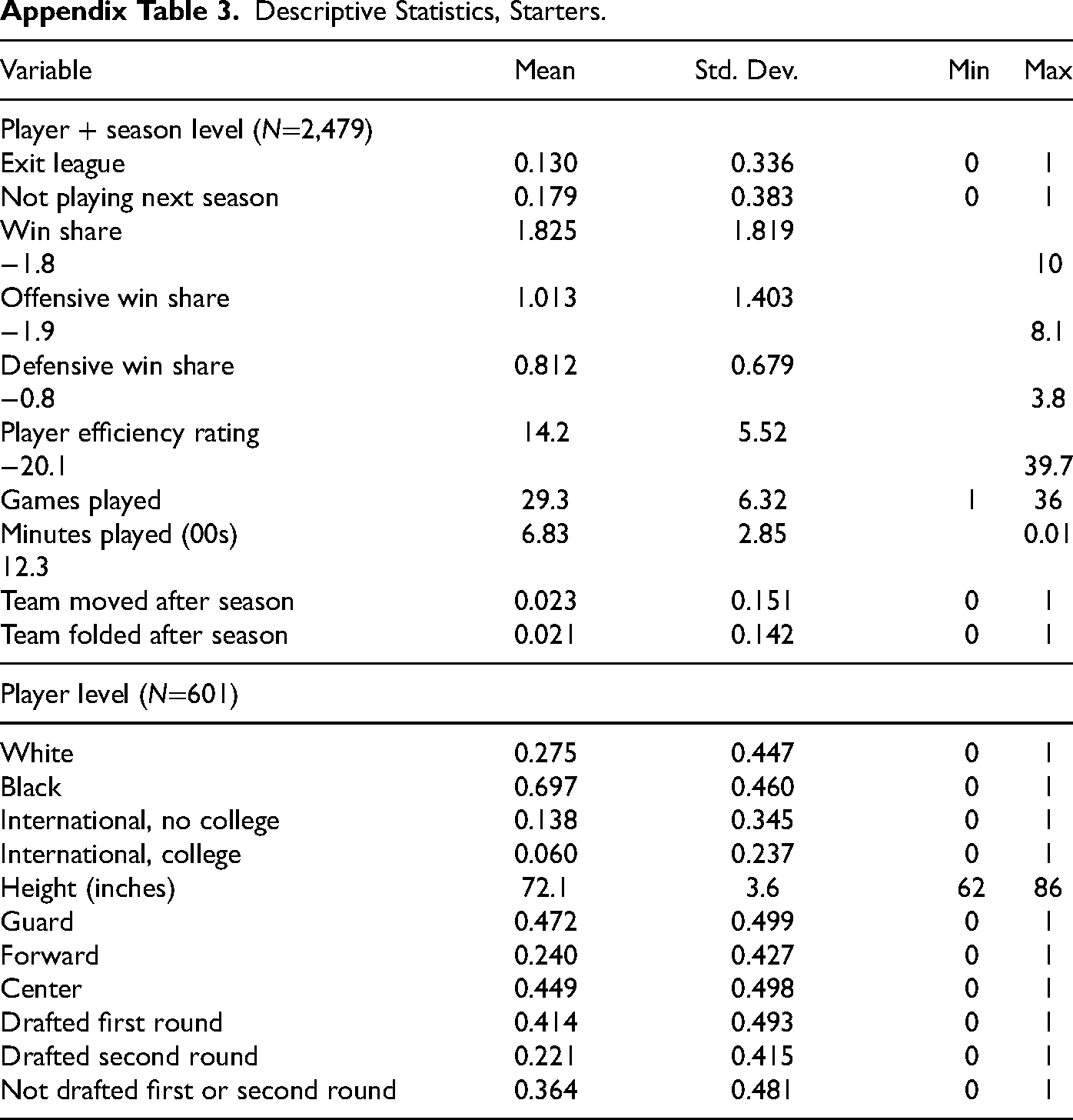
Descriptive Statistics, Starters.

Variable	Mean	Std. Dev.	Min	Max
Player + season level (N=2,479)
Exit league	0.130	0.336	0	1
Not playing next season	0.179	0.383	0	1
Win share	1.825	1.819	−1.8	10
Offensive win share	1.013	1.403	−1.9	8.1
Defensive win share	0.812	0.679	−0.8	3.8
Player efficiency rating	14.2	5.52	−20.1	39.7
Games played	29.3	6.32	1	36
Minutes played (00s)	6.83	2.85	0.01	12.3
Team moved after season	0.023	0.151	0	1
Team folded after season	0.021	0.142	0	1
Player level (N=601)
White	0.275	0.447	0	1
Black	0.697	0.460	0	1
International, no college	0.138	0.345	0	1
International, college	0.060	0.237	0	1
Height (inches)	72.1	3.6	62	86
Guard	0.472	0.499	0	1
Forward	0.240	0.427	0	1
Center	0.449	0.498	0	1
Drafted first round	0.414	0.493	0	1
Drafted second round	0.221	0.415	0	1
Not drafted first or second round	0.364	0.481	0	1

The logit marginal effects are nearly identical across the different specifications for experience (Table 3, columns 1–4). White players and international players, particularly those who did not play U.S. college basketball, are more likely to exit the league, with larger marginal effects among international players for the more common outcome of a career break.

The next sensitivity analysis concerns the measures of performance, as shown in Columns 5 and 6 of Table 3. Again, the three measures of performance are: (1) win share (Column 1, as in Table 2), (2) offensive and defensive win share (Column 5), and (3) player efficiency rating (Column 6). All models include linear and quadratic terms for performance. The marginal effect for White players is somewhat larger in the two models with win-share (around 0.04) compared with the model including player efficiency (roughly 0.033). The marginal effects for international players vary little across the specifications of productivity. More productive players are less likely to exit.¹¹

The last sensitivity test in Table 3 is the use of a probit model (as in Groothuis & Hill, 2013) for comparison with the logit results presented so far. Column 7 includes marginal effects for probit models. The results are very similar between the probit model marginal effects in Column 7 and the logit marginal effects in Column 1. In the career exit model, for example, the marginal effect for White is 0.046 in the probit model (Column 7) compared with 0.043 in the logit model (Column 1), whereas the marginal effects are 0.040 for both specifications when the outcome is a career break.

So far, no distinction is made between players who typically start games and those who play less regularly during the entire season. In the final sensitivity analysis, the sample contains only players who started at least one game in the season. By doing so, the focus is on the employment dynamics for the highest-achieving players. Appendix Table 3 shows the descriptive statistics for this sample of starters. The table illustrates that career exits and career breaks are less common among starters, consistent with lower turnover among the most productive workers. Only 13% of observations among starters represent a career exit, compared with 23% for the full sample (Table 1). For career breaks, the means are 18% for starters and 28% for all observations (Table 1). Among starters, 27.5% are White, nearly 14% are international with no U.S. college experience, and 6% are international with U.S. college experience.

Table 4 presents the results for starters, using the preferred specification with win share as the measure of productivity and a set of dummy variables to measure experience. The likelihood of a career exit is 0.035 higher for Whites, and the likelihood of a career break is 0.040. Thus, the higher turnover among White players does not appear to be driven by players with the least labor-force attachment. Among starters, international players with no U.S. college experience are 5.3 percentage points more likely to exit the WNBA entirely and are 13.0 percentage points more likely to take a career break. However, international players with U.S. college basketball experience have similar employment dynamics as U.S.-born players. Although the size of the marginal effect varies, the pattern of results is similar between starters and all players.

Table 4.

Determinants of Career Exits and Breaks, Starters.

	Career Exit			Career Break
	Marginal	Standard		Marginal	Standard
	Effect	Error		Effect	Error
White	0.035	0.016	**	0.040	0.020	**
International, no college	0.053	0.024	**	0.130	0.035	***
International, college	0.018	0.032		0.019	0.039
Win share	−0.039	0.008	***	−0.034	0.009	***
Games played	0.002	0.001		0.002	0.001	*
Minutes played (00s)	−0.036	0.004	***	−0.040	0.005	***
Height (inches)	−0.008	0.003	***	−0.007	0.003	**
Center	0.049	0.024	**	0.057	0.030	*
Forward	0.028	0.015	*	0.020	0.019
Drafted first round	−0.040	0.015	***	−0.036	0.019	*
Drafted second round	−0.022	0.015		−0.001	0.019
Team moved after season	−0.004	0.043		0.000	0.051
Team folded after season	−0.043	0.037		−0.005	0.056
Pseudo R-sq	0.273			0.214
Mean dependent variable	0.130			0.179

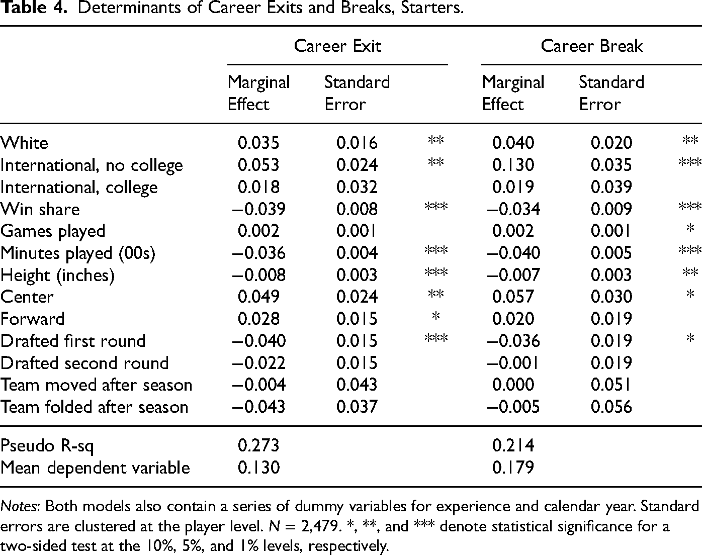
Notes: Both models also contain a series of dummy variables for experience and calendar year. Standard errors are clustered at the player level. N = 2,479. *, **, and *** denote statistical significance for a two-sided test at the 10%, 5%, and 1% levels, respectively.

Conclusion

This paper provides novel evidence on the employment dynamics of WNBA players. The determinants are similar for the likelihood that a player leaves the WNBA permanently or for a career break defined as not returning for the following season. White players are more likely to leave, as are international players with no U.S. college experience. More productive players and players drafted in the first round are less likely to leave. These results are robust to alternate measurements of experience and productivity, whether measured as a logit or a probit, as well as for starters or for all players.

How do the results for the WNBA compare with the NBA, where salaries are orders of magnitude larger? In contrast to the positive association of exit for Whites in the WNBA, previous work finds no systematic relationship between race and career exit in the NBA (Groothuis & Hill, 2004, 2013, 2018).¹² To explore potential explanations for this result, I look beyond sports to the general workforce. Perhaps White players have better job options outside of the WNBA, as Albrecht et al. (2015) and Fisher and Houseworth (2017) document higher wages for White women than for Black women. Although job mobility among college-educated workers is similar between White and non-White women (Alon & Tienda, 2005),¹³ recent work shows some evidence of increases in perceived job insecurity (Kuroki, 2016) and a desire to switch jobs in the presence of perceived discrimination (Ng et al., 2021) for White women relative to non-White women. But further research (with better data) is needed to discern the extent to which general patterns in the labor market explain the WNBA's higher exit rates for White women.

Turning to international players, such players with no U.S. college basketball have higher propensities of exiting the league in both the NBA (Groothuis & Hill, 2018) and the WNBA (Table 2). Also in both leagues, more productive players and players drafted in the first round have lower exit rates. The goodness of fit, as measured by the pseudo R-squared, is around 0.3 in Table 3 and in Groothuis and Hill (2018) for the NBA. Thus, aside from race, the NBA and WNBA have broadly similar determinants of employment dynamics.

Although this paper provides an initial look at employment determinants in women's basketball, much more research in women's sports is needed. The literature is nearly non-existent regarding the determinants of employment and salaries in women's sports. Further work in the WNBA is also essential. I make no distinctions among the possible reasons for nonemployment, such as injury, motherhood, or personal reasons. Due to a lack of data, I am unable to study the determinants of WNBA salaries or explain the higher exit rate for White women. Future work could also look at employment and salaries in other basketball leagues, especially given that most WNBA players also play in other leagues. In basketball and other women's sports, many unanswered questions remain.

Footnotes

Declaration of Conflicting Interests

The author declared no conflicts of interest with respect to the research, authorship, and/or publication of this article.

Funding

The author received no financial support for the research, authorship, and/or publication of this article.

ORCID iD

Christopher Jepsen

Notes

Author biography

Christopher Jepsen is a professor of economics at University College Dublin. Within sports economics, his current research interests include the determinants of salaries and employment for football.

Appendix

Table 3.

Sensitivity Analysis, Selected Coefficients.

	Preferred	Experience as Polynomial			Alternate Performance		Probit
	Logit	Third Order	Fourth Order	Fifth Order	OWS, DWS	PER	Model
	(1)	(2)	(3)	(4)	(5)	(6)	(7)
Career exit
White	0.043***	0.042***	0.042***	0.042***	0.042***	0.034**	0.046***
International, no coll.	0.042*	0.043*	0.044*	0.044*	0.044*	0.046**	0.046**
International, college	0.025	0.025	0.024	0.024	0.025	0.023	0.027
Win share	−0.067***	−0.068***	−0.068***	−0.068***			−0.062***
OWS					−0.060***
DWS					−0.086***
PER						−0.005***
Pseudo R-squared	0.324	0.321	0.322	0.322	0.324	0.323	0.324

Career break
White	0.040**	0.039**	0.039**	0.039**	0.038**	0.033**	0.040**
International, no coll.	0.119***	0.119***	0.120***	0.120***	0.121***	0.125***	0.122***
International, college	0.053*	0.053*	0.052*	0.052*	0.053*	0.050*	0.053*
Win share	−0.052***	−0.052***	−0.052***	−0.052***			−0.050***
OWS					−0.045***
DWS					−0.064**
PER						−0.005***
Pseudo R-squared	0.285	0.284	0.284	0.284	0.285	0.287	0.280

Notes: The models differ in how experience is specified, how performance is measured, or functional form, as noted in the column headings. All models also contain the control variables listed in Table 2 and its notes as well as controls for experience, and a series of dummy variables for season and calendar year. Standard errors are clustered at the player level. Full results for these specifications are available from the author upon request. LPM = linear probability model; OWS = offensive win share; DWS = defensive win share; PER = player efficiency rating. N= 3,573. *, **, and *** denote statistical significance for a two-sided test at the 10%, 5%, and 1% levels, respectively.

References

Ajilore

(2014). Do white NBA players suffer from reverse discrimination? Economics Bulletin, 34(1), 558–566.

Albrecht

van Vuuren

Vroman

(2015). The Black-White wage gap among young women in 1990. Labour Economics, 33(1), 66–71. https://doi.org/10.1016/j.labeco.2015.02.006

Alon

Tienda

(2005). Job mobility and early career wage growth of White, African-American, and Hispanic Women. Social Sciences Quarterly, 86(5), 1196–1217. https://doi.org/10.1111/j.0038-4941.2005.00342.x

Berger

M. C.

Black

D. A.

(1998). The duration of medicaid spells: An analysis using flow and stock samples. The Review of Economics and Statistics, 80(4): 667–674. https://doi.org/10.1162/003465398557762

Berger

M. C.

Black

D. A.

Scott

. (2004). Is there job lock? Evidence from the pre-HIPAA era. The duration of medicaid spells: An analysis using flow and stock samples. Southern Economic Journal 70(4), 953–976. https://doi.org/10.2307/4135282

Brown

R. W.

Todd Jewell

(2006). The marginal revenue product of a women's college basketball player. Industrial Relations, 45(1), 96–101. https://doi.org/10.1111/j.1468-232X.2006.00415.x

Depken

C. A.

Williams

Wilson

D. P.

(2011). From the hardwood to the gridiron to the dorm: Influences on attendance to women's collegiate basketball. International Journal of Sport Finance, 6(1), 3–22.

Dey

M. S.

(1997). Racial differences in national basketball association players’ salaries: A new look. The American Economist, 41(2), 84–90. https://doi.org/10.1177/056943459704100211

Elvira

M. M.

Zatzick

C. D.

(2002). Who’s displaced first? The role of race in layoff decisions. Industrial Relations, 41(2), 329–361. https://doi.org/10.1111/1468-232X.00248

10.

Eschker

Perez

S. J.

Siegler

M. V.

(2004). The NBA and the influx of international basketball players. Applied Economics, 36(10), 1009–1020. https://doi.org/10.1080/0003684042000246713

11.

Fisher

J. D.

Houseworth

C. A.

(2017). The widening Black-White wage gap among women. Labour, 31(3), 288–308. https://doi.org/10.1111/labr.12099

12.

Gius

Johnson

(1998). An empirical investigation of wage discrimination in professional basketball. Applied Economics Letters, 5(11), 703–705. https://doi.org/10.1080/135048598354168

13.

Gokcekus

Godet

Ramsey

(2010). Are women more predictable than men? Applied Economics, 42(4–6), 641–645. https://doi.org/10.1080/00036840701704451

14.

Groothuis

P. A.

Hill

J. R.

(2013). Pay discrimination, exit discrimination, or both? Another look at an old issue using NBA data. Journal of Sports Economics, 14(2), 171–185. https://doi.org/10.1177/1527002511418515

15.

Groothuis

P. A.

Hill

J. R.

(2018). Career duration in the NBA: Do foreign players exit early? Journal of Sports Economics, 19(6), 873–883. https://doi.org/10.1177/1527002517690789

16.

Groothuis

P. A.

Richard Hill

(2004). Exit discrimination in the NBA: A duration analysis of career length. Economic Inquiry, 42(2), 341–349. https://doi.org/10.1093/ei/cbh065

17.

Harris

Berri

D. J.

(2015). Predicting the WNBA draft: What matters most from college performance? International Journal of Sport Finance, 10(4), 299–309.

18.

Harris

Berri

D. J.

(2016). If you can't pay them. Play them: Fan preferences and own-race bias in the WNBA. International Journal of Sport Finance, 11(3), 247–261.

19.

Hill

(2021). Tournament incentives and performance: Evidence from the WNBA. Contemporary Economic Policy, 39(4), 882–900. https://doi.org/10.1111/coep.12530

20.

Hill

J. R.

(2004). Pay discrimination in the NBA revisited. Quarterly Journal of Business and Economics, 43(1–2), 81–92.

21.

Hill

J. R.

Groothuis

P. A.

(2017). Is there a wage premium or wage discrimination for foreign-born players in the NBA? International Journal of Sport Finance, 12(3), 204–221.

22.

Hoang

Rascher

(1999). The NBA, exit discrimination, and career earnings. Industrial Relations, 38(1), 69–91. https://doi.org/10.1111/0019-8676.00110

23.

Humphreys

B. R.

(2000). Equal pay on the hardwood: The earnings gap between male and female NCAA division I basketball coaches. Journal of Sports Economics, 1(3), 299–307. https://doi.org/10.1177/152700250000100306

24.

Johnson

Minuci

(2020). Wage discrimination in the NBA: Evidence using free agent signings. Southern Economic Journal, 87(2), 517–539. https://doi.org/10.1002/soej.12461

25.

Kahn

L. M.

Shah

(2005). Race. Compensation, and contract length in the NBA, 2001–2002. Industrial Relations, 44(3), 444–462. https://doi.org/10.1111/j.0019-8676.2005.00394.x

26.

Kahn

L. M.

Sherer

P. D

. (1988). Racial differences in professional basketball players’ compensation. Journal of Labor Economics 6(1), 40–61. https://doi.org/10.1086/298174

27.

Kuroki

(2016). An analysis of perceptions of job insecurity among White and Black workers in the United States: 1977–2012. Review of Black Political Economy, 43(3–4), 289–300. https://doi.org/10.1007/s12114-016-9237-6

28.

McGoldrick

Voeks

(2005). 'We got game!': An analysis of win/loss probability and efficiency differences between the NBA and WNBA. Journal of Sports Economics, 6(1), 5–23. https://doi.org/10.1177/1527002503262649

29.

Naito

Takagi

(2017). Is racial salary discrimination disappearing in the NBA? Evidence from Data During, 1985–2015. International Review of Applied Economics 31(5), 651–669. https://doi.org/10.1080/02692171.2017.1303037

30.

E. S.

Sears

G. J.

Bakkaloglu

(2021). White and minority employee reactions to perceived discrimination at work: Evidence of White fragility? International Journal of Manpower, 42(4), 661–682. https://doi.org/10.1108/IJM-12-2019-0535

31.

Paul

R. J.

Weinbach

A. P.

(2014). Market efficiency and behavioral biases in the WNBA betting market. International Journal of Financial Studies, 2(2), 193–202. https://doi.org/10.3390/ijfs2020193

32.

Robst

VanGilder

Coates

C. E.

Berri

D. J.

(2011). Skin tone and wages: Evidence from NBA free agents. Journal of Sports Economics, 12(2), 143–156. https://doi.org/10.1177/1527002510378825

33.

Rosas

Orazem

P. F.

(2014). Is self-sufficiency for women's collegiate athletics a hoop dream? Willingness to pay for men's and women's basketball tickets. Journal of Sports Economics, 15(6), 579–600. https://doi.org/10.1177/1527002512462706

34.

Schroeffel

J. L.

Magee

C. S. P.

(2012). Own-Race bias among NBA coaches. Journal of Sports Economics, 12(2), 130–151. https://doi.org/10.1177/1527002511402758

35.

Toma

(2017). Missed shots at the free-throw line: Analyzing the determinants of choking under pressure. Journal of Sports Economics, 18(6), 539–559. https://doi.org/10.1177/1527002515593779

36.

Yang

C.-H.

Lin

H.-Y.

(2012). Is there salary discrimination by nationality in the NBA? Foreign talent or foreign market. Journal of Sports Economics, 13(1), 53–75. https://doi.org/10.1177/1527002510391617

37.

Zax

J. S.

(1989). Quits and race. Journal of Human Resources, 24(3), 469–493. https://doi.org/10.2307/145824

Determinants of Career Exits and Career Breaks in Women's Professional Basketball

Abstract

Keywords

Introduction

Relationship to Literature

Data and Descriptive Statistics

Methods

Results

Main Results

Collective Bargaining

Sensitivity Analysis

Conclusion

Footnotes

Declaration of Conflicting Interests

Funding

ORCID iD

Notes

Author biography

Appendix

References