Analysis of Beibu Gulf tidal zone exposure on properties of carbon steel

Abstract

Marine tidal zone is a corrosive environment that has a negative impact on carbon steel. This research investigates the change of mechanical properties and corrosion behaviour of carbon steel specimens subjected to field exposure test and simulation test for 12 and 6 months, respectively. The corrosion behaviour of carbon steel exposed to real marine tidal zone and simulation environment was discussed through morphological observation and corrosion kinetics analysis, in order to reveal the essential reason for the degradation of its mechanical properties. Then the tensile test was performed on the corroded specimens and true stress–strain curves were obtained. In addition, regression equations were derived for the mechanical properties as a function of the degree of corrosion degradation and a constitutive model with time factor for corroded carbon steel is proposed.

Introduction

Many marine constructions, such as the risers and the legs of the platform, are exposed to the marine environment. However, it's well-known that seawater is an aggressive corrosive environment, where the corrosion problem suffered by carbon steel (CS) is serious, threatening the safety of structures on durability and even causing structure failure.^1–3 Therefore, the corrosion of CS in marine environments has attracted much attention from scholars and the study of corrosion of CS in seawater environments began as early as the 1940s.^4,5

The corrosion of CS in the marine environment is affected by many factors.⁶⁻¹⁰ The chloride ion also is a key factor affecting marine corrosion, as its high concentration promotes the formation of β-FeOOH, which can affect the morphology of the rust layer and the corrosion rate.^11–13 And scholars found that the corrosion degree of CS in tidal zone ¹⁰ is higher than that in the marine atmosphere zone ⁹ and immersion zone. ⁸ Moreover, it was confirmed that the corrosion rate is associated with the wet/dry cycle and the height of the steel strip exposed to the tidal zone.^6,7 Therefore, it is necessary to conduct research on the corrosion behaviour of tidal zone in specific seas with their different tidal cycles, temperatures and salinity.

Differences in corrosion behaviour and corrosion mechanisms lead to differences in the degradation of the mechanical properties of CS. The monotonic tensile test of corroded CS shows that the modulus of elasticity, yield stress, tensile strength and total elongation of CS decreases with the increase of corrosion degree.^14–16 Other mechanical properties of CS such as fatigue strength^17,18 and impact toughness^19,20 can also be negatively affected by corrosion. The loss of cross-section is a main factor affecting the strength of CS, while the increase in surface roughness caused by uneven corrosion results in the decrease of plasticity and toughness.^14–16 Furthermore, different constitutive models of corroded steels under different corrosive environments were proposed,^{15,16,21–23} in order to predict the mechanical properties of CS corroded in the different corrosive environments for a long time.

However, both the corrosion mechanism and the mechanical properties of corroded CS are mainly studied in the accelerated tests,^24–27 while the corrosion of CS under field tests especially exposed to the tidal zone are rarely mentioned. The effect of the wave on the corrosion of CS in marine tidal zones is often overlooked. Moreover, most of the damaged previous constitutive models of corroded steels constitutive models are not closely related to the real marine environment and corrosion time, only related to the degree of corrosion. Thus, it is indispensable to explore the corrosion behaviour and the mechanical property deterioration of CS corroded in the real marine tidal zone.

Based on previous research result ²⁸ on the corrosion behaviour of CS in the Beibu Gulf tidal zone of our research group, this article investigates the impact of corrosion behaviour on mechanical properties of CS in the Beibu Gulf tidal zone through field exposure test and simulation test. The difference in corrosion behaviour of CS in two environments is discussed and the mechanical properties of corroded specimens are tested to summarise the degradation law which is thought to be related to corrosion behaviour. Besides, the damage constitutive model of CS based on the field exposure test is proposed, which can predict the mechanical properties of CS corroded at different times in the tidal zone of Beibu Gulf.

Material and methods

Test material

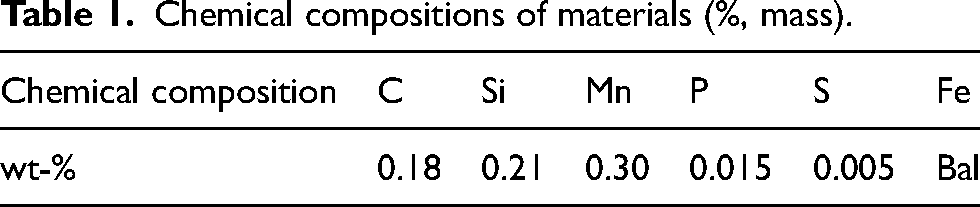
The Q235B CS (Carbon Steel) was applied in the tests, in which Q represents yield stress, 235 represents the yield stress value of steel, the unit is MPa, and B is the deoxidation symbol for semi-killed steel. The chemical compositions of CS are provided in Table 1. All specimens were machined from the same steel plate and polished to smoothness. The geometry and dimension of the specimens is given in Figure 1. Moreover, the specimens were ultrasonically cleaned with acetone, then rinsed with distilled water, dried with a blower, and stored for 24 h, respectively, before use.

Figure 1.

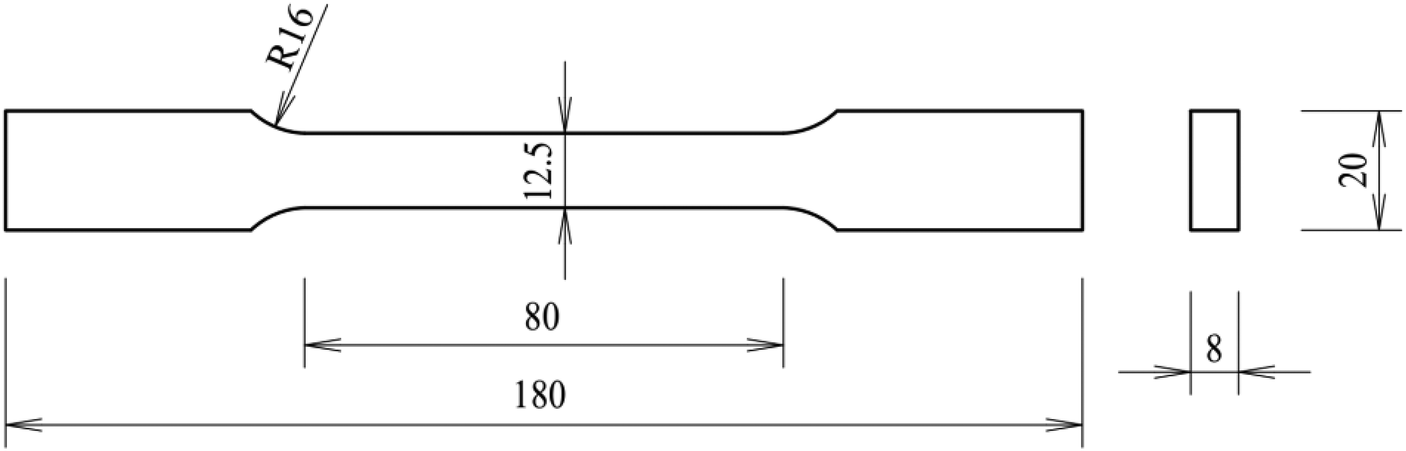
The dimensions of dog-bone specimens (unit: mm).

Table 1.

Chemical compositions of materials (%, mass).

Chemical composition	C	Si	Mn	P	S	Fe
wt-%	0.18	0.21	0.30	0.015	0.005	Bal

Marine exposure test and simulation test

The field exposure test site is situated at a Beibu Gulf port (21°29′ N, 109°05′ E) in Beihai City, China, which is located in the subtropical monsoon climate zone, and the environmental condition mentioned in the authors’ previous research. ²⁸ Specimens were fixed to the self-made frames and placed in the tidal zone where the dry-wetting time proportion is 5:1, as shown in Figure 2. Three specimens were retrieved for subsequent corrosion behaviour research and mechanical properties test every 30 days, from August 2020 to August 2021.

Figure 2.

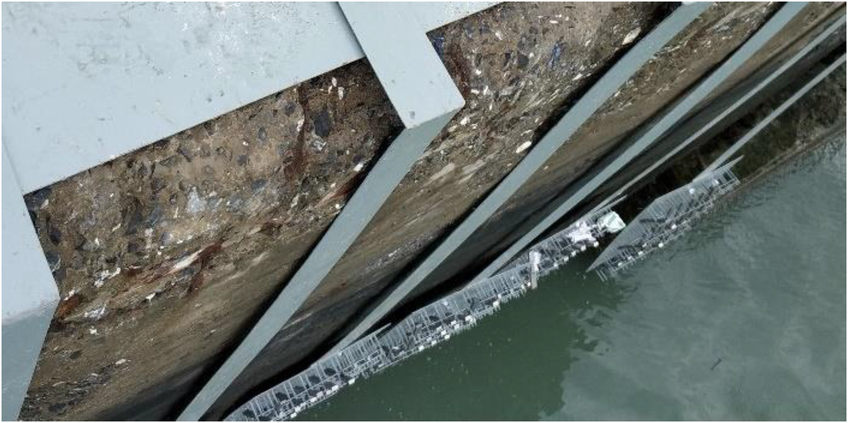
The field exposure test site.

Figure 3 shows the tidal experimental device for the simulation test. By using a time relay and two water level sensors to control the working time and speed of the water pump and switch two water pumps to pump water between the test tank and the seawater storage tank, the corrosion of CS under the influence of tidal fluctuations in the marine tidal environment is simulated. Artificial seawater with the same chloride iron concentration and pH as the exposure site environment was used. An aerator and a temperature controller were used to ensure that the oxygen content in the aqueous solution was sufficient and the water temperature was stable at 25 °C. In order to speed up the corrosion process in the simulation test, the tidal period was set to 1 h with the same dry-wetting time proportion. The same number of specimens was placed in the simulated tidal zone. The simulation test lasted for 180 days, and the specimens were retrieved every 30 days and then the same mechanical properties test also occurred on these specimens.

Figure 3.

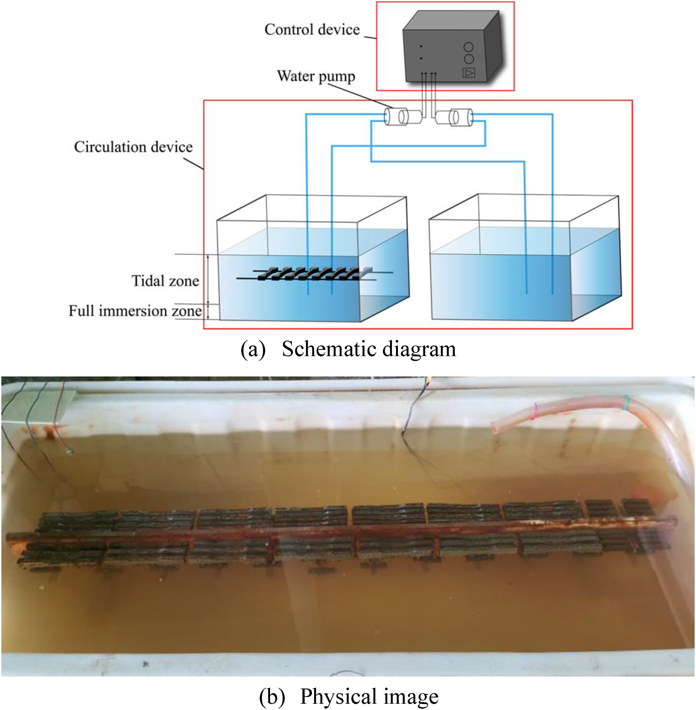
Experimental device for simulating tidal zone.

Characterisation of corrosion

The macro-morphology of specimens was taken with a high-definition digital camera to investigate the corrosion on the surface of CS. The rust layers of the specimens were carefully removed with an art blade, and the micro-morphology of the rust layers was observed and analysed with a Zeiss evo18 scanning electron microscope (SEM).

Measurement of the corrosion loss

Before the tests, the original mass of each specimen, w₀ (in g), was measured by a precision balance. After retrieving the corroded specimens from the exposure location and simulated the condition periodically, these specimens were immersed in a specific solution (500 mL hydrochloric acid + 500 mL distilled water + 3.5 g hexamethylenetetramine) in an ultrasonic cleaner at 25 °C for about 15 min to remove the corrosion products. Then, the specimens were cleaned with acetone and dried to get the final mass, w_t (in g).

Tensile testing

The static tensile test for all specimens was performed via an MTS-809.25 Electro-hydraulic servo tension and torsion combination fatigue testing machine from the United States, as shown in Figure 4. All tests were conducted according to ISO 6892-1:2009 ²⁹ at room temperature. During each test, the specimen was fully clamped at both ends and stretched up to fracture under displacement control at a constant rate of 2 mm/min. The MTS632.68F-08 extensometer was used to track the deformation, and it was dismantled when getting the ultimate load. The extensometer data and load–displacement curve were automatically recorded by the data-acquisition system.

Figure 4.

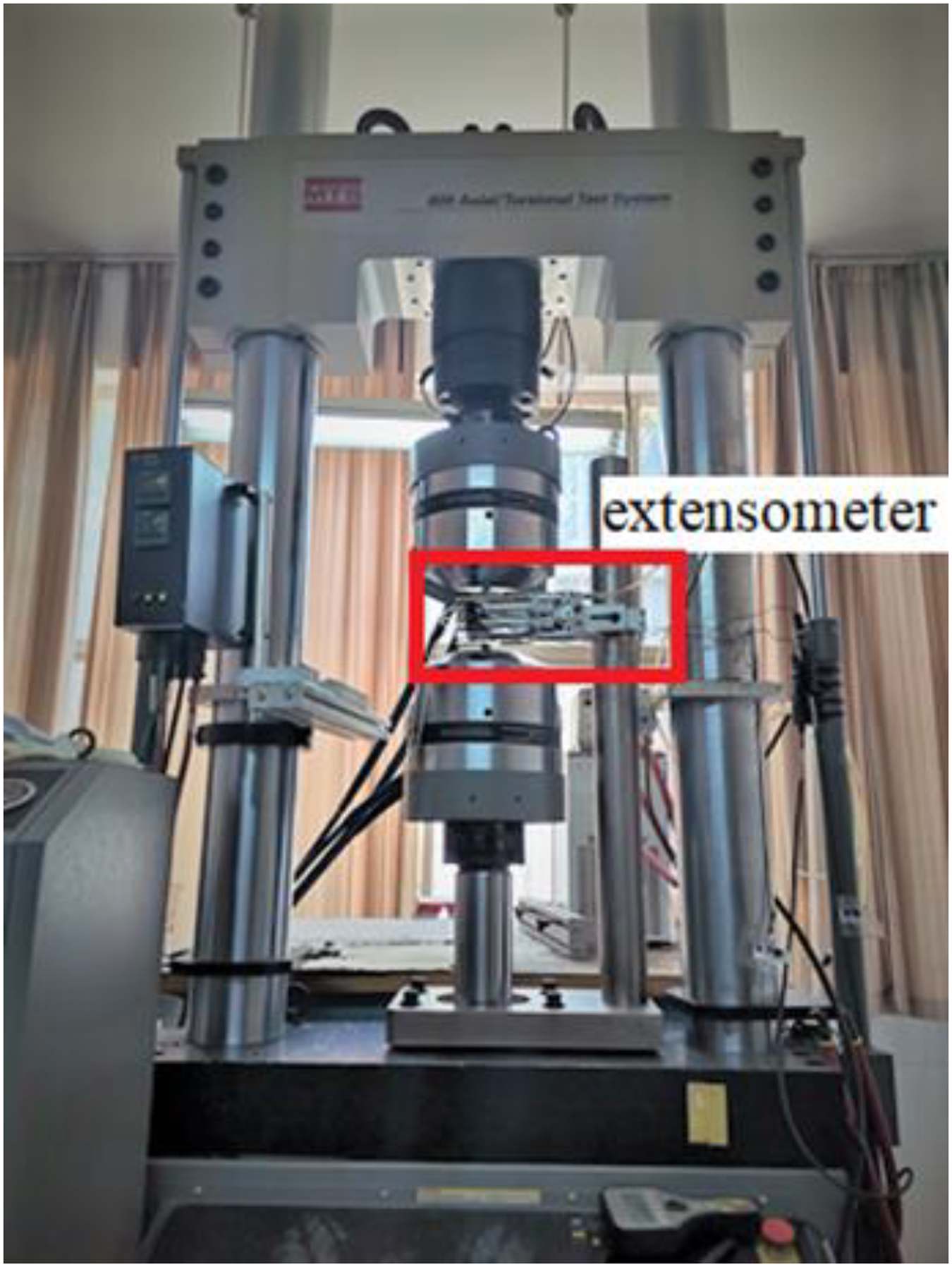
Tensile testing machine.

Experimental results and discussion

Corrosion characteristics

Mass loss and corrosion rate

As mentioned, specimens were weighed with the same digital balance before and after exposure to a corrosive environment in order to determine the mass loss of the corroded specimens. The mass loss ratio D_w and corrosion rate CR are used as reference values to characterise the corrosion degree of the tested specimens and the values are listed in Table 2. The mass loss ratio D_w is calculated through equation (1)

$$D\mathrm{w}={\displaystyle \frac{w_0-w_{\mathrm{t}}}{w_0}.}$$

(1)

Table 2.

Mass loss ratio and corrosion rate of corroded specimens.

Condition	Specimen	D w	CR	Condition	Specimen	D w	CR
		(%)	(μm a−1)			(%)	(μm a−1)
Field exposure test	F-2-1a	9.20	1563.93	Simulation test	S-1-1	9.26	3149.70
	F-2-2	7.23	1229.98		S-1-2	9.30	3163.31
	F-4-1	14.74	1253.67		S-2-1	15.47	2513.23
	F-4-2	14.74	1253.67		S-2-2	16.04	2605.88
	F-6-1	13.98	792.43		S-3-1	16.75	1855.42
	F-6-2	16.91	958.49		S-3-2b	18.22	2017.64
	F-8-1	19.24	818.06		S-4-1	18.16	1544.25
	F-8-2	13.83	587.99		S-4-2	18.64	1585.04
	F-10-1	17.42	592.50		S-5-1	19.51	1326.66
	F-10-2	20.61	700.95		S-5-2	20.08	1365.89
	F-12-1	21.98	622.89		S-6-1	22.34	1323.55
	F-12-2	21.12	598.64		S-6-2	20.57	1166.28

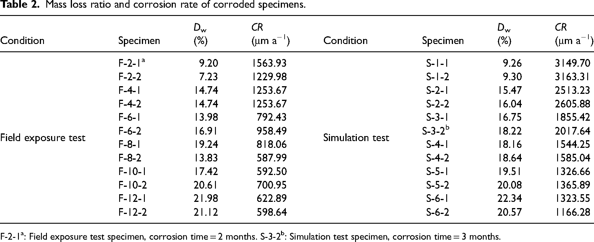
F-2-1^a: Field exposure test specimen, corrosion time = 2 months. S-3-2^b: Simulation test specimen, corrosion time = 3 months.

Average corrosion rate CR is expressed as the annual average corrosion thickness loss with equation (2)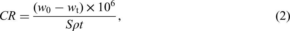

$$CR={\displaystyle \frac{(w_0-w_{\mathrm{t}})\times {10}^6}{S\rho t},}$$

(2)

where CR is the corrosion rate (in μm a⁻¹), (w₀–w_t) means the mass loss of specimens (in g), S is specimen area (in m²), ρ represents the density of CS (in gm⁻³), and t signifies the corrosion time (in a).

Corrosion kinetics

A large number of studies have shown that the corrosion process of steel is conformed to the power function,^30,31 which can represent the development trend of corrosion behaviour of metals:

$$D_{\mathrm{w}}=A{t}^n,$$

(3)

where t is corrosion time (in days), both A and n are constants. It is generally believed that A is related to external environmental factors such as temperature and salinity, and the value of n is a factor for judging the compactness of the rust layer structure, which can be used to indicate the development trend of corrosion. Figure 5(a) presents the variation of the average mass loss ratio with corrosion time after fitting. The high R² values indicate that the corrosion kinetics of CS in the tidal zone is consistent with equation (3). The n values for the two tests are < 1, which represents under both testing conditions the CS corrosion was a deceleration process. The results also indicate that the corrosion kinetics of CS during the simulation environment is basically the same as that in marine tidal environments. What's more, the much higher A value of the simulation test shows that CS has a higher initial corrosion rate, and the value of n of the field exposure test is slightly higher, which indicates that the rust layers are sparser and more unprotected, and the CS has a higher subsequent corrosion trend.

Figure 5.

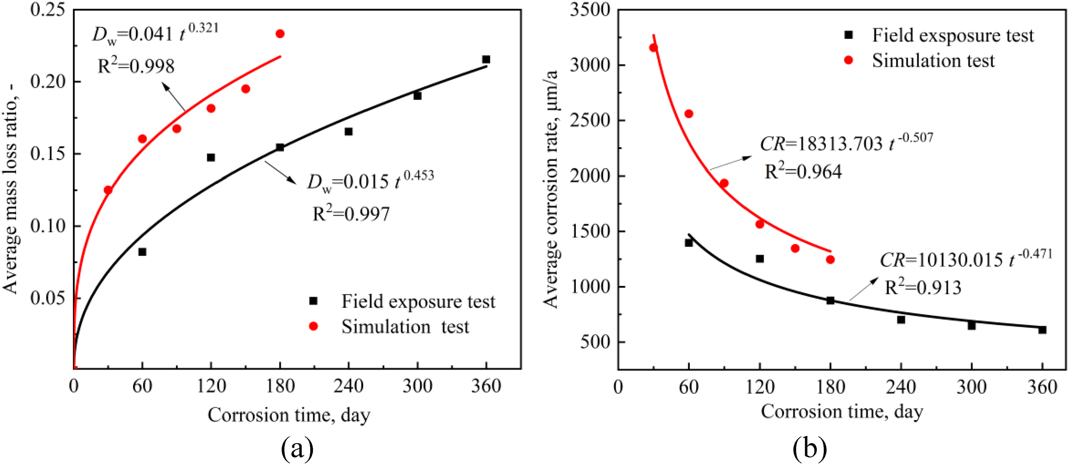
Corrosion kinetics curves for (a) mass loss ratio, (b) corrosion rate under two test conditions.

The fact that the corrosion rate decreases sharply and then slowly with corrosion time can be seen in Figure 5(b), indicating that the protective rust layer can be formed on CS during the corrosion process but its protection is limited. With the progress of corrosion, the corrosion rate difference of CS in the two environments gradually decreases, but it will not disappear within a certain period of time.

Macroscopic morphologies of the rust layers

The macro-morphology of the rust layers surface of specimens of different corrosion times for the field exposure test and simulation test are captured via digital camera is shown in Figures 6 and 7, respectively. In both corrosive environments, the rust layer was getting increasingly thicker as the corrosion proceeded. It may be that chlorine ions promoted the rapid growth of corrosion product particles, making the surface corrosion products lose and easily detached. Additionally, after 180 days for the exposure test and 90 days for the simulation test, the corrosion products formed two layers, the outer layer is lighter in colour, loose and easy to peel off, while the inner layer is darker and denser. After the formation of a dense inner rust layer, the corrosion rate decreases significantly, which can be proved by the variation of CR with corrosion time (Figure 5(b)).

Figure 6.

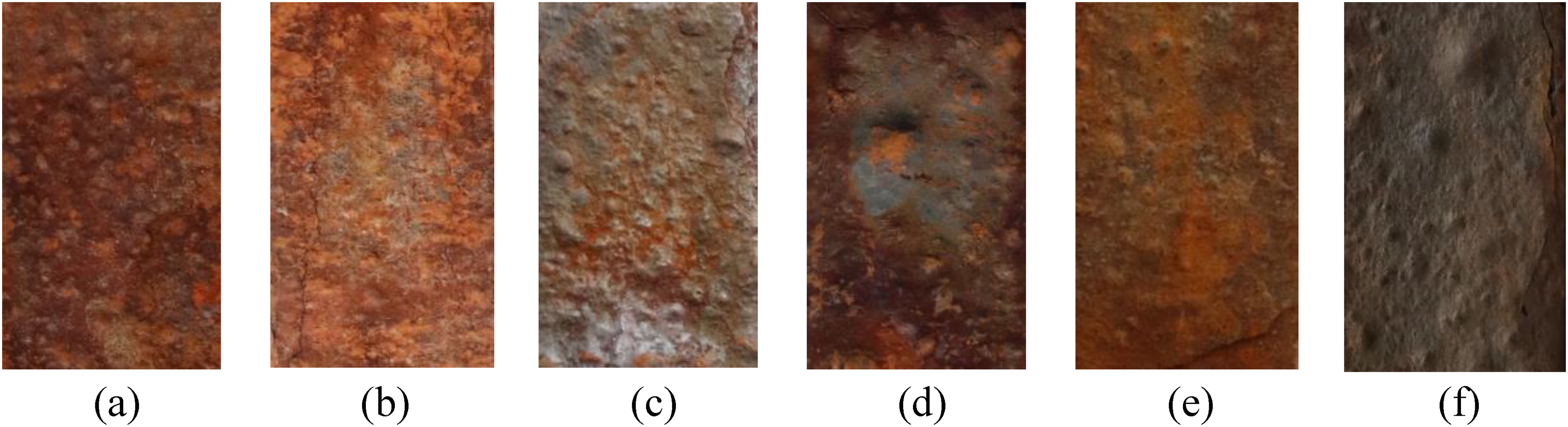
Surface morphologies of the rust layers for field exposure test after different corrosion times: (a) 60 days, (b) 120 days, (c) 180 days, (d) 240 days, (e) 300 days, and (f) 360 days.

Figure 7.

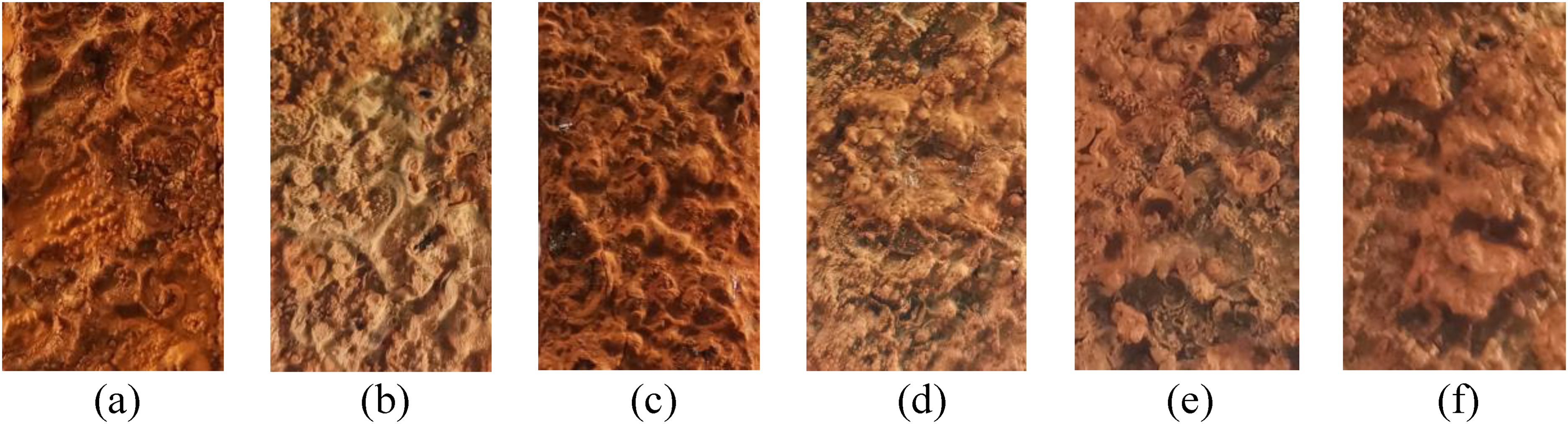
Surface morphologies of the rust layers for simulation test after different corrosion times: (a) 30 days, (b) 60 days, (c) 90 days, (d) 120 days, (e) 150 days, and (f) 180 days.

Figure 6 shows that the rust layers of specimens are stripped of the loose products due to wave washing, the overall appearance of the rust layers is more uniform and the colour is darker and reddish-black. However, the loose part of the outer rust layer is retained and silted up in the upper layer in the simulation environment without wave washing, so the rust layer is thicker and reddish-brown as shown in Figure 7. This is the reason why the n value of the corrosion kinetics equation of CS in the real marine condition is higher.

Moreover, there are many bulges that can be seen in Figures 6 and 7, and adjacent small bulges were connected to become a large one with the corrosion time. This is an obvious phenomenon, indicating that non-uniform corrosion is occurring. As seawater is rich in chlorine ions, and other electrolytes, the drying process, will crystallise in the CS substrate, resulting in inconsistent drying speed of the surface. The corrosion rate of those first crystallised locations is faster, because of the high salt concentration and sufficient oxygen. And then due to the water retention of the loose rust layer, the first place to corrode will remain relatively fast corrosion rate, so that more corrosion products are produced, causing rust layer to bulges.

Microscopic morphologies of the rust layers

Figures 8 and 9 present the front micro-morphologies of the rust layers and the microstructure of some corrosion products via SEM (Scanning Electron Microscope). The SEM surface morphology of CS in the field exposure test is smoother than that in the simulation test due to the erosion of seawater.

Figure 8.

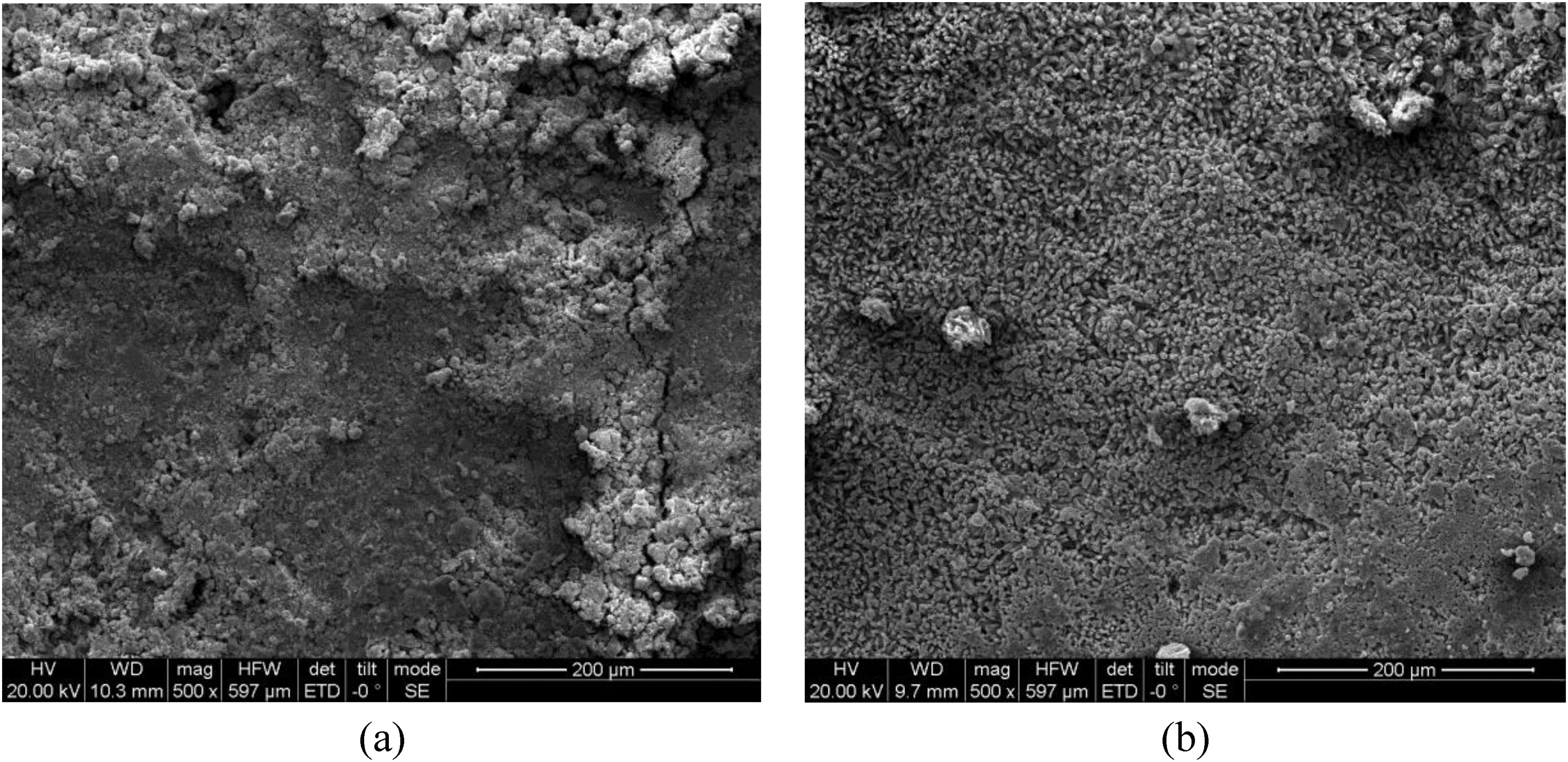
The SEM surface morphology of CS corrosion products for field exposure test after (a) 60 days and (b) 180 days.

Figure 9.

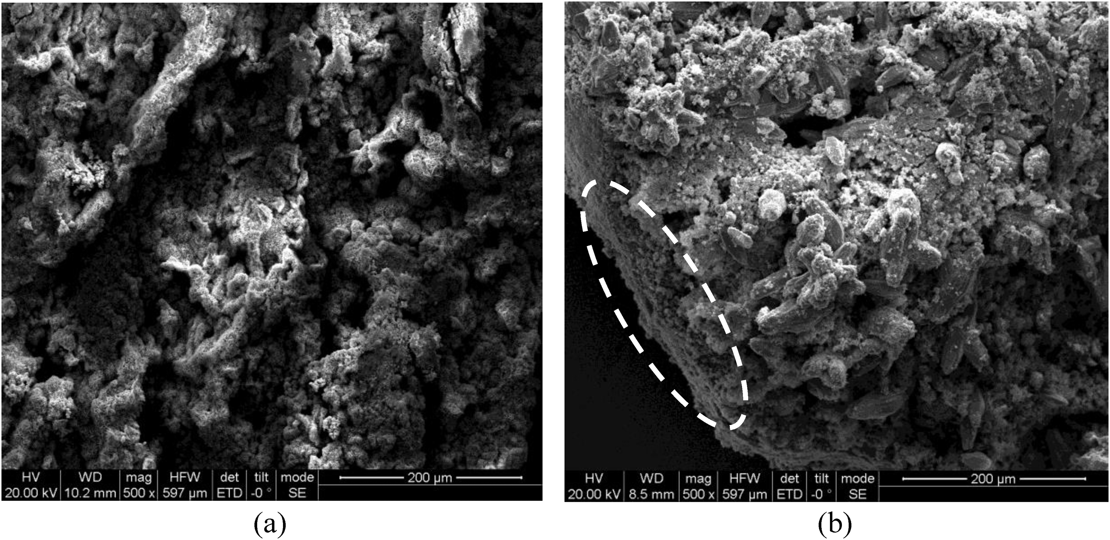
The SEM surface morphology of CS corrosion products for simulation test after (a) 30 days and (b) 90 days.

Figure 8(a) shows that the corrosion products packed on the surface of CS are loose and porous, after 60 days of exposure. With the accumulation of corrosion products, it can be seen that the corrosion products become dense after the formation of two rust layers (Figure 8(b)).

Figure 9(a) shows the CS surface micro-morphologies in the early and middle stages of corrosion in the simulation test. In the early stage of corrosion, a large number of corrosion products accumulate on the CS surface. As the corrosion progresses, corrosion products continue to accumulate due to the absence of waves, but the corrosion products will also form a denser inner rust layer (elliptical mark in Figure 9(b)), which can provide sufficient protection.

Morphologies of steel substrates

The macro-morphology of the CS surface after removing the rust layers is presented in Figure 10. After 60 and 30 days of corrosion in the real marine tidal environment and simulation environment, respectively, the CS surface is uniformly covered with dense small and shallow corrosion pits (Figure 10(a) and (b)). With the increase of corrosion time, the corrosion degree of CS increases significantly, and so does the size and depth of the low shallow corrosion pits (Figure 10(c) and (d)). In late corrosion, larger pits increase and some of the pits are interconnected and eventually become one large erosion pit (Figure 10(e) and (f)). The above results denote that the corrosion modes of CS under a tidal environment are uniform corrosion and non-uniform corrosion. The pitting of CS occurs first and then evolves into uniform corrosion. The theory of the intrusion mechanism of chloride ions in the passive film suggests that the mechanical stress of pores and impurities in steel is the main cause of passivation film failure. ³² Therefore, the local large corrosion pits in the substrate are caused by the destruction of the local passive film by the enriched Cl^–. The substrate is continuously eroded, and the pits show a tendency to aggregate in the later stage of the test. Another reason for this phenomenon is that in the middle and late stages of corrosion, as the rust layer thickens and becomes dense, water, oxygen and chlorine ions can only reach the inner rust layer through cracks in order to contact the CS substrate and this partial contact can eventually lead to non-uniform corrosion of CS.

Figure 10.

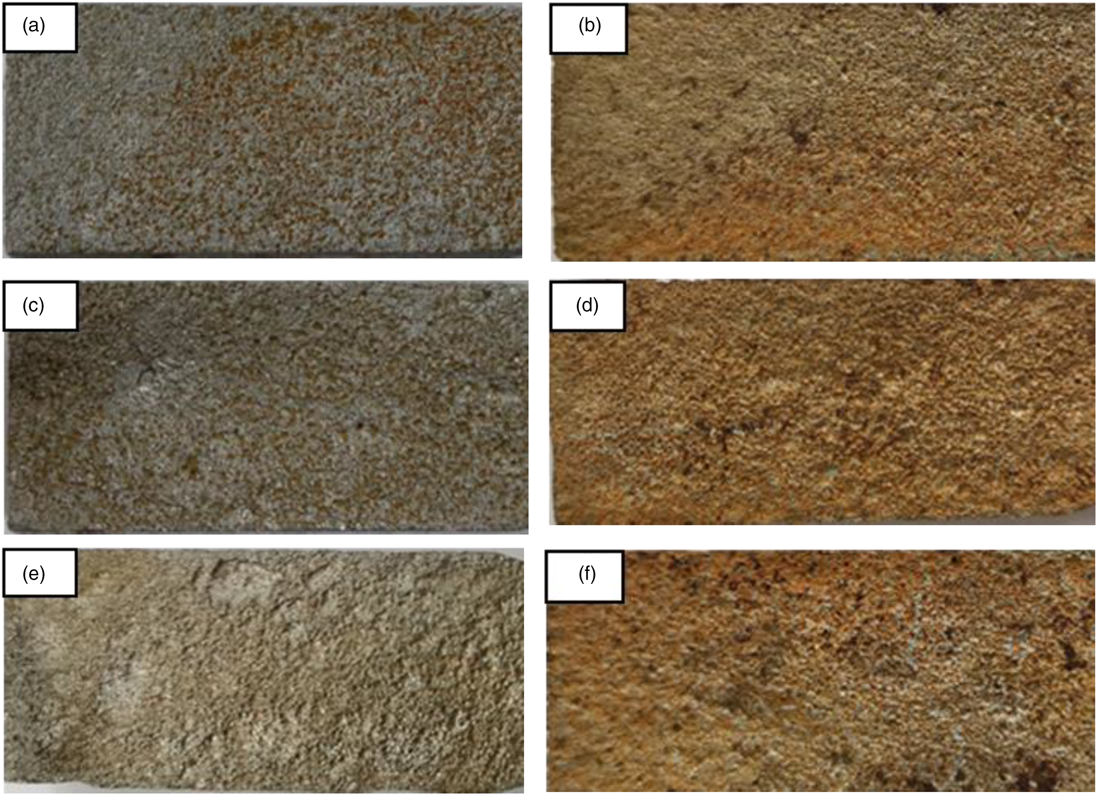
Macro-morphology of the steel surface after removing the corrosion products: in real marine condition (a, c, e); in accelerated condition (b, d, f).

As can be seen in Figure 10(e) and (f), the corrosion pits on the CS substrate under a real marine tidal environment are larger and deeper than those under simulation environment, indicating that it has a higher degree of non-uniform corrosion. We speculate that the time of one dry cycle may be one of the main factors affecting the substrate non-uniform corrosion. Because the accelerated condition has a short dry/wet cycle time, the longtime of wetting makes the CS more inclined to occur uniform corrosion. In addition, the rust layer of the accelerated test specimens without wave impact is more uniform and thicker, and the distribution of corrosion pits of the specimens is more uniform than that of the real marine corrosion specimens.

Mechanical properties

True stress–strain curves

Tensile tests were conducted on two non-corroded specimens and twelve groups of specimens corroded in two corrosion conditions for different periods of time to determine the effects of corrosion degradation on the mechanical properties. In conventional engineering tensile tests, the engineering stress and strain are determined by the measured loads and deflections and expressed by σ_e and ɛ_e, respectively,

$${\sigma }_{\mathrm{e}}={\displaystyle \frac{P}{A_0},{\epsilon }_{\mathrm{e}}={\displaystyle \frac{\delta }{L_0},}}$$

(4)

where δ is the controlled displacement, P is the load corresponding to displacement, A₀ is the original specimens’ cross-sectional area of the specimen and L₀ is the scale length.

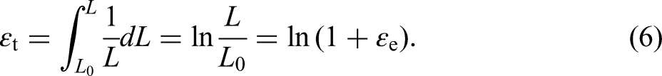
However, the cross-sectional area and scale length of the specimen would change during the tensile process. The stress and strain calculated using the varying cross-sectional area and scale length are called true stress and true strain, denoted as σ_t and ɛ_t, respectively,

$${\sigma }_{\mathrm{t}}={\displaystyle \frac{P}{A}={\displaystyle \frac{P}{A_0}(1+{\epsilon }_{\mathrm{e}})={\sigma }_{\mathrm{e}}(1+{\epsilon }_{\mathrm{e}}),}}$$

(5)

$${\epsilon }_{\mathrm{t}}={\int }_{L_0}^L{\displaystyle \frac{1}{L}}dL=\ln {\displaystyle \frac{L}{L_0}=\ln (1+{\epsilon }_{\mathrm{e}}).}$$

(6)

When the true stress, σ_t is plotted against the strain, ɛ_t, the curve obtained is known as the true stress–strain curve.

In this article, the true stress–strain curves are established for all tested specimens. Figure 11 shows the typical true stress–strain curves of the non-corroded specimen and the corroded specimens exposed to two corrosive environments. The results illustrate that the curve shape of corroded specimens still strongly resembles that of the non-corroded specimen. However, after corrosion, the mechanical properties degrade observably. With the increase of corrosion time, the ultimate stress and ultimate strain of specimens decrease gradually. In particular, specimens F-10-2 and S-1-1 seem to have fractured without reaching the expected strength, as the pitting corrosion effect is the main cause of this phenomenon. As can be seen from the local magnification of the yield stage in Figure 11, corrosion can reduce the yield strength of CS, while it does not seem to affect the length of the yield terrace within a certain corrosion degree, except for specimen S-2-1. The yield terrace of specimen S-2-1 disappears, and the stress becomes larger at the beginning of plastic deformation, which may be affected by the decrease in carbon content due to microbial corrosion.

Figure 11.

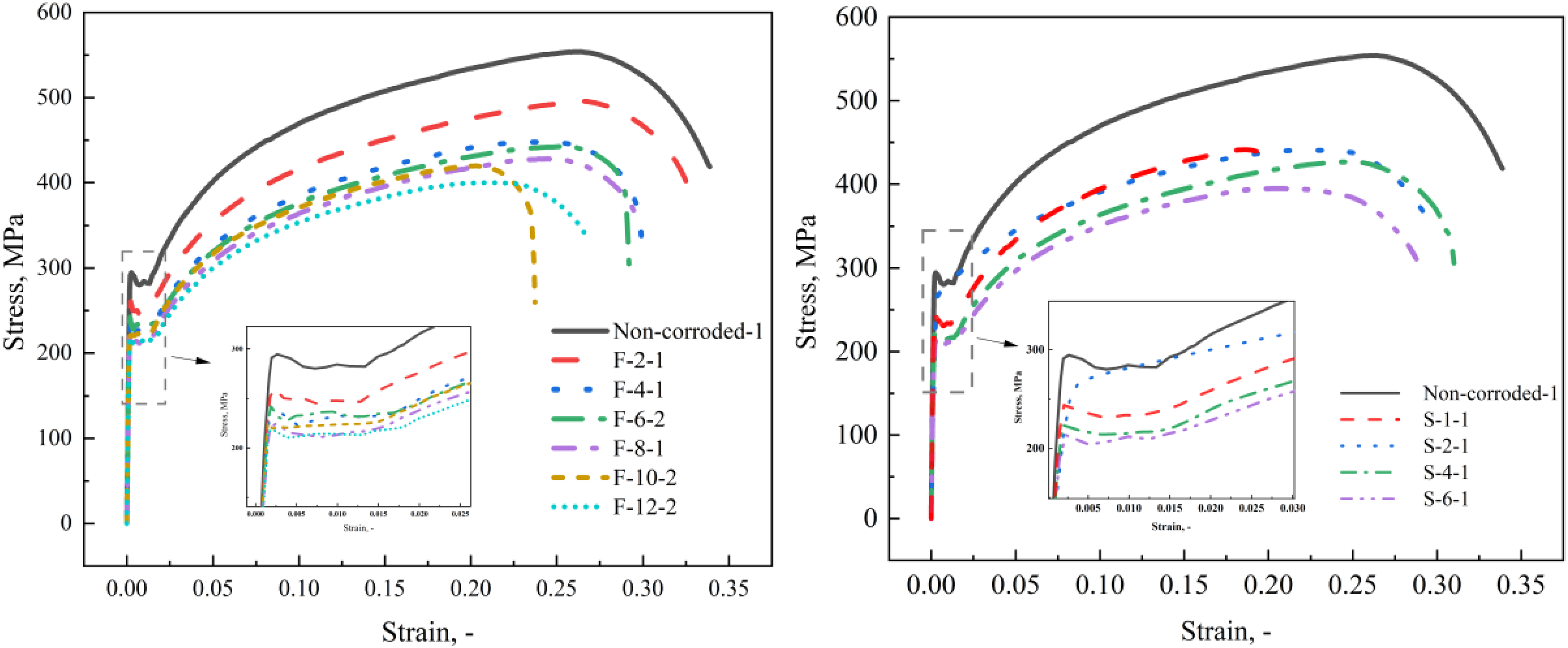
Typical true stress–strain curve of corroded specimens for (a) field exposure test and (b) simulation test.

It has been observed in Figure 12 that the true stress–strain curves of corroded specimens with similar degrees of corrosion degradation under both corrosion conditions nearly overlap in the portion before necking. In contrast, after necking, the stresses of field exposure specimens decrease more rapidly, resulting in lower elongation at break. What causes this phenomenon is that the larger and deeper pits caused by non-uniform corrosion on the CS surface exposed to the real marine tidal zone led to faster initiation and propagation of cracks.

Figure 12.

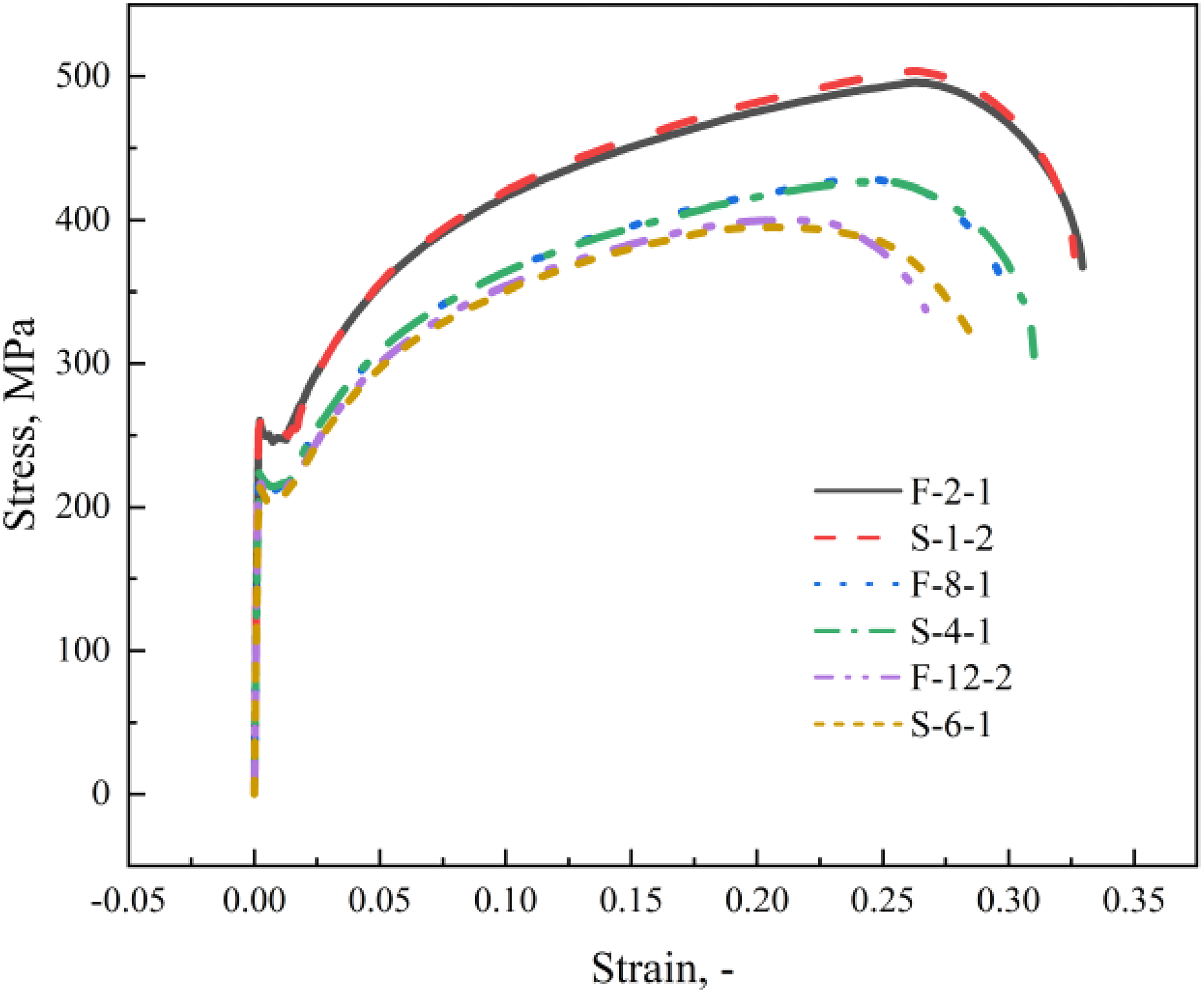
Typical true stress–strain curves for specimens with similar corrosion degrees under two corrosive environments.

Effect of corrosion on the mechanical properties

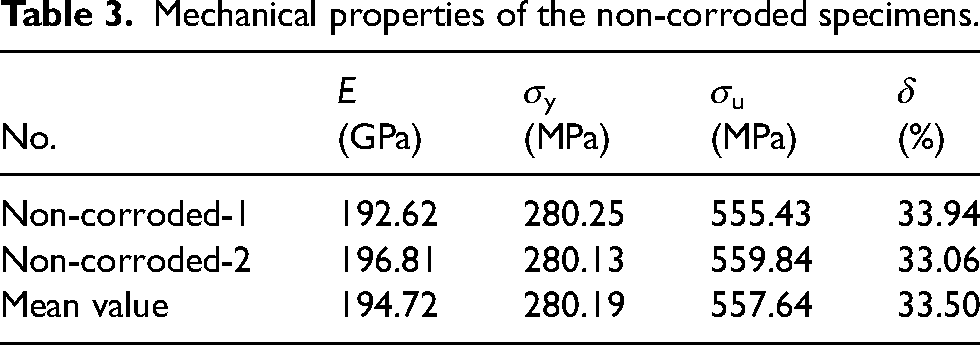
True stress–strain curves of all specimens were analysed to obtain mechanical properties such as modulus of elasticity E, yield strength σ_y, tensile strength σ_u, and total uniform elongation δ. The Average value of mechanical properties (E₀, σ_y0, σ_u0, δ₀) for non-corroded specimens are obtained and listed in Table 3. It is especially important to note that the mechanical properties of specimens F-2-1 and S-1-2 whose D_w just approximately equal to 10% had been a significant reduction. When D_w exceeds 20%, such as in specimens F-12-2 and S-6-1, the yield strength and tensile strength of corroded specimens drop by more than 30% and 40%, respectively, which indicates that uniform corrosion has a great influence on the mechanical properties of CS. Besides, the significant decrease in elongation (more than 20%) means that the mechanical properties are also affected by non-uniform corrosion.

Table 3.

Mechanical properties of the non-corroded specimens.

No.	E	σ y	σ u	δ
	(GPa)	(MPa)	(MPa)	(%)
Non-corroded-1	192.62	280.25	555.43	33.94
Non-corroded-2	196.81	280.13	559.84	33.06
Mean value	194.72	280.19	557.64	33.50

Figures 13 and 14 show the variations in mechanical properties with different mass loss ratios of all the specimens. For the sake of discussion, all the parameters are normalised with respect to the mean value of the non-corroded cases. For all mechanical property parameters, the decreasing trend of the field exposure test is always higher than that of the simulation test, which means that the corrosion under a real tidal environment has a greater influence on CS.

Figure 13.

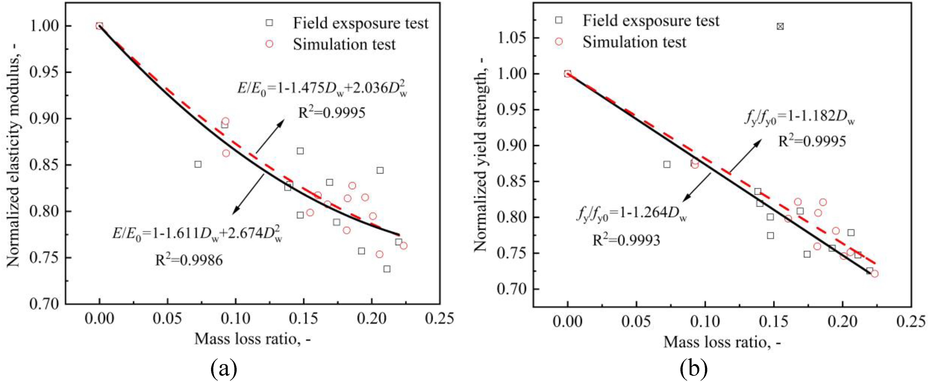
Variation of (a) modulus of elasticity and (b) yield strength with mass loss ratio.

Figure 14.

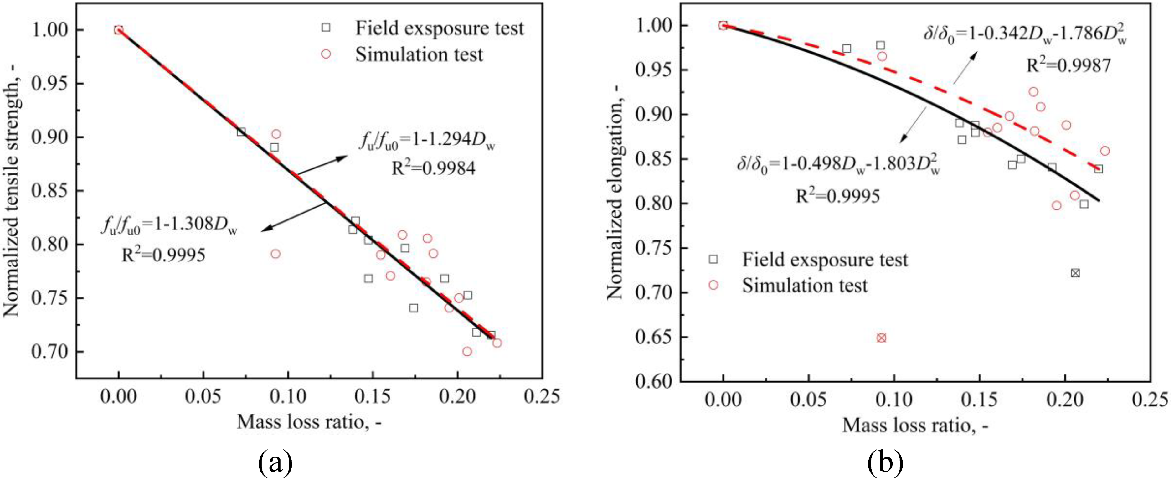
Variation of (a) tensile strength and (b) total uniform elongation with mass loss ratio.

The elasticity modulus E, an important mechanical property of CS, was calculated based on the fitting results of the initial linear portion of the true stress–strain curves (Figure 13(a)). The elasticity modulus results fit to a quadratic regression curve with a coefficient of determination R²= 0.8674 and 0.9302 for field exposure test specimens and simulation test specimens, respectively.

Field exposure test specimens:

$$E_{\mathrm{s}}/E_{\mathrm{s}0}=1-1.611D_{\mathrm{w}}+2.674D_{\mathrm{w}}^2.$$

(7)

Simulation test specimens:

$$E_{\mathrm{s}}/E_{\mathrm{s}0}=1-1.475D_{\mathrm{w}}+2.036D_{\mathrm{w}}^2.$$

(8)

Possible stress in the tensile elastic stage and at this stress level plastic deformation begins. Q235B CS has a remarkable yielding phenomenon, the lower yield point is taken as the yield strength. According to the true stress–strain curves of all corroded specimens, the yield stress is obtained and presented in Figure 13(b). When fitting the yield stress data, the yield stress of specimen S-2-1 is considered to be failure data, but it is still shown in the figure with a forked symbol. A strong linear correlation of the experimental results was found by linear fitting with the coefficient of determination R²= 0.9993 and 0.9995.

Field exposure test specimens:

$${\sigma }_{\mathrm{y}}/{\sigma }_{\mathrm{y}0}=1-1.264D_{\mathrm{w}}.$$

(9)

Simulation test specimens:

$${\sigma }_{\mathrm{y}}/{\sigma }_{\mathrm{y}0}=1-1.182D_{\mathrm{w}}.$$

(10)

Tensile strength is considered to be one of the most important mechanical properties of CS and is an important reference in the structural design process. In fact, tensile strength is the maximum possible stress in tension and at this stress level necking starts. The experimental results of the tensile strength are given in Figure 14(a). As can be observed, the linear trend fits the experimental data very well with the coefficient of determination R²= 0.9995 and 0.9984.

Field exposure test specimens:

$${\sigma }_{\mathrm{u}}/{\sigma }_{\mathrm{u}0}=1-1.308D_{\mathrm{w}}.$$

(11)

Simulation test specimens:

$${\sigma }_{\mathrm{u}}/{\sigma }_{\mathrm{u}0}=1-1.294D_{\mathrm{w}}.$$

(12)

The elongation, index of plastic properties, which is defined as the ratio of the extension of gauge length to gauge length, is shown in Figure 14(b). The values become discrete with the increase of corrosion degree, which is caused by the enlargement and uneven distribution of corrosion pits. It can be seen from Figure 14(b), that the linear trend also fits the results (except for specimens F-10-2 and S-1-1) with the coefficient of determination R²= 0.9995 and 0.9987.

Field exposure test specimens:

$$\delta /{\delta }_0=1-0.498D_{\mathrm{w}}-1.803D_{\mathrm{w}}^2.$$

(13)

Simulation test specimens:

$$\delta /{\delta }_0=1-0.342D_{\mathrm{w}}-1.786D_{\mathrm{w}}^2.$$

(14)

After corrosion, all the mechanical properties mentioned above declined with the increase of corrosion degree. The decreasing trends of elastic modulus, yield strength and tensile strength of CS under the two corrosion conditions are very close, indicating that they are mainly affected by degradation of cross-section due to uniform corrosion. In contrast, the elongation of CS corroded in real marine tidal conditions decreases faster than that of the simulation test, which indicates that the elongation is dominantly subject to the influence of corrosion pits caused by non-uniform corrosion.

Stress–strain curve modelling

To predict the performance of engineering structures subjected to a corrosive environment, it is necessary to research the deterioration of material properties. The main content of this section is to establish an equivalent stress–strain curve of CS specimens based on tensile tests of corroded specimens exposed to the real marine tidal environment as a function of the corrosion time.

As shown in Figure 15, the three-stage constitutive model is applied in the monotonic loading curve of the specimens: the first stage is the elastic segment (O-Y); the second one is the yielding segment (Y-H); the third one is the hardening segment (H-U). The Johnson–Cook constitutive model can well characterise the flow stress during the reinforcement phase of the true stress–strain curve, which is expressed as equation (15):

$${\sigma }_{\mathrm{eq}}=({\sigma }_{\mathrm{y}}+K{\epsilon }_{\mathrm{eq}}^n)(1+C\ln {\dot{\epsilon }}^{*})(1\text{-}{T}^{*m}),$$

(15)

where σ_eq is the equivalent stress, ε_eq is the equivalent plastic strain, σ_y is the yield stress under reference deformation conditions, K is the strength coefficient, n is the strain hardening index, C is the strain rate strengthening coefficient, $\dot{\epsilon }*$ is the dimensionless strain rate, T* is the homologous temperature and m is the thermal softening coefficient. In this article, the specimens were subjected to static uniaxial tensile tests at room temperature, $\dot{\epsilon }*=1$ , $m=0$ . Then the Johnson–Cook model can be simplified as equation (16):

$${\sigma }_{\mathrm{eq}}={\sigma }_{\mathrm{y}}+K{\epsilon }_{\mathrm{eq}}^n.$$

(16)

Figure 15.

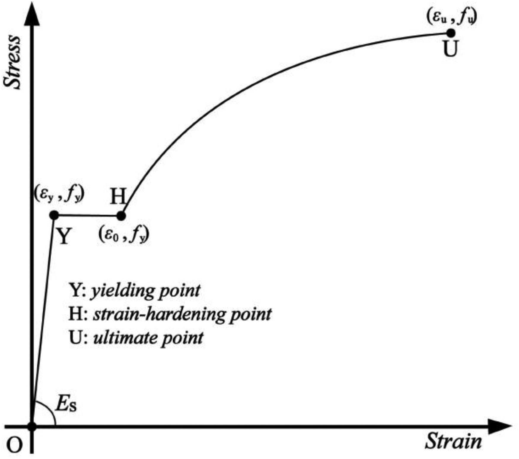
Three-stage constitutive model.

The mathematical expressions of the three-stage model are shown in equation (17):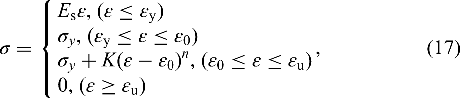

$$\sigma =\{\begin{array}{c}{E}_{\mathrm{s}}\epsilon ,(\epsilon \le {\epsilon }_{\mathrm{y}})\\ {\sigma }_y,({\epsilon }_{\mathrm{y}}\le \epsilon \le {\epsilon }_0)\\ {\sigma }_y+K(\epsilon -{\epsilon }_0{)}^n,({\epsilon }_0\le \epsilon \le {\epsilon }_{\mathrm{u}})\\ 0,(\epsilon \ge {\epsilon }_{\mathrm{u}})\end{array},$$

(17)

where E_s is the modulus of elasticity, σ_y is the yield stress, ε_y is the yield strain, ε_u is the ultimate strain, ε₀ the is strain for the hardening point and ε_u is the ultimate strain.

The hardening stage of the true stress-strain curves for the specimens with different corrosion levels are fitted by equation (17) and the corresponding strain hardening index, n and strength coefficient K are obtained and listed in Table 4, which also shows other parameters values of constitutive model obtained from the tensile test results. It can be noticed that the strain hardening index n is much more dispersed than the K value. The linear regression analysis of the parameter n results in a coefficient R²= 0.098, indicating no significant dependence on D_w and, therefore, no regression is provided, with an average value of 0.470 for n. As shown in Figure 16, the regression analysis of K and ε_u are performed as equations (18) and (19):

$$K=543.664-798.332D_{\mathrm{w}}+1284.083D_{\mathrm{w}}^2,$$

(18)

$${\epsilon }_{\mathrm{u}}=0.259+0.062D_{\mathrm{w}}-1.269D_{\mathrm{w}}^2.$$

(19)

So far, the three-stage model can be expressed in equation (20):

$$\sigma =\{\begin{array}{cc}(1-1.611D_{\mathrm{w}}+2.674D_{\mathrm{w}}^2)E_{\mathrm{s}0}\epsilon ,& (\epsilon \le {\epsilon }_{\mathrm{y}})\\ (1-1.264D_{\mathrm{w}}){\sigma }_{y0},& ({\epsilon }_{\mathrm{y}}\le \epsilon \le {\epsilon }_0)\\ (1-1.264D_{\mathrm{w}}){\sigma }_{y0}+(543.664\text{-}798.332D_{\mathrm{w}}+1284.083D_{\mathrm{w}}^2)(\epsilon -{\epsilon }_0{)}^{0.47},& ({\epsilon }_0\le \epsilon \le {\epsilon }_{\mathrm{u}})\\ 0.& (\epsilon \ge {\epsilon }_{\mathrm{u}}).\end{array}$$

(20)\hfill

Figure 16.

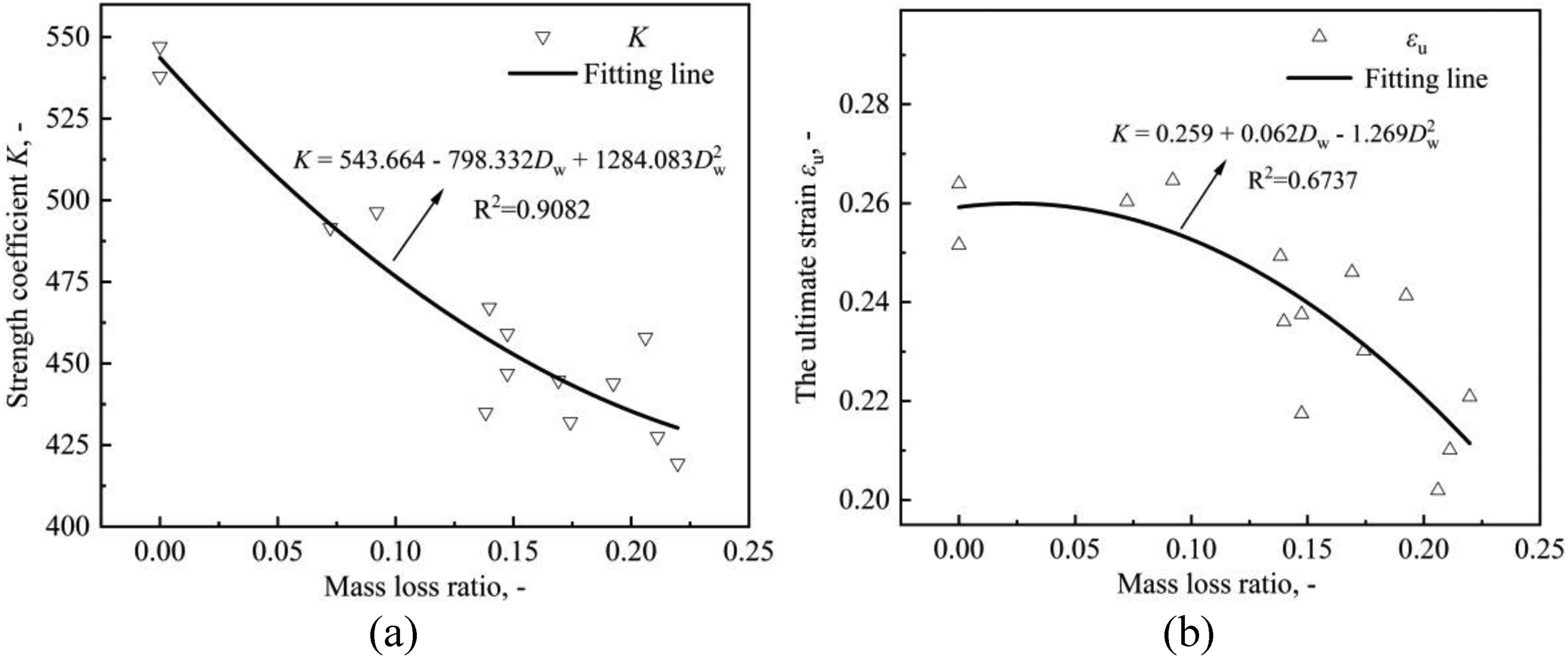
Variation of (a) strength coefficient K and (b) the ultimate strain ε_u with mass loss ratio.

Table 4.

Parameters value of the constitutive model obtained from the tensile test results.

No.	ε y	ε 0	ε u	K	n
Non-corroded-1	0.00147	0.01393	0.26397	537.965	0.447
Non-corroded-2	0.00142	0.01451	0.25072	547.033	0.435
F-2-1	0.00140	0.01225	0.26266	496.371	0.457
F-2-2	0.00147	0.01686	0.26038	491.567	0.448
F-4-1	0.00144	0.01675	0.23750	459.148	0.474
F-4-2	0.00128	0.01675	0.21742	446.922	0.487
F-6-1	0.00142	0.01563	0.23605	467.131	0.465
F-6-2	0.00139	0.01745	0.24603	444.779	0.489
F-8-1	0.00143	0.01533	0.24132	443.897	0.473
F-8-2	0.00145	0.01978	0.24931	434.958	0.489
F-10-1	0.00136	0.01325	0.23011	432.033	0.470
F-10-2	0.00132	0.01504	0.20194	457.940	0.479
F-12-1	0.00136	0.01765	0.22086	419.339	0.487
F-12-2	0.00145	0.01819	0.21011	427.509	0.483

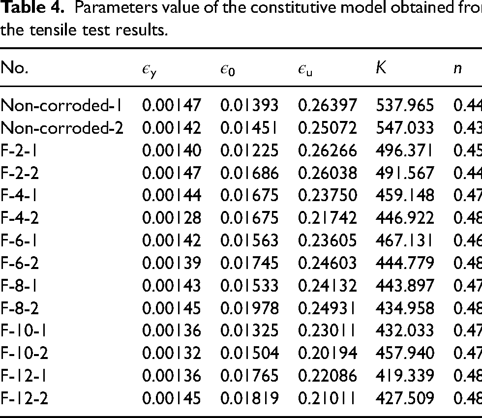
Similar to n, neither the yielding strain ε_y nor the hardening strain ε₀ is significantly dependent on D_w. So, ε_y can be determined by σ_y/E_s, and ε₀ can be determined by the average of the ratio of ε₀ to ε_y for specimens: ε₀= 11.328ε_y. The constructed stress–strain curves for the degree of degradation of 0%–30% are shown in Figure 17.

Figure 17.

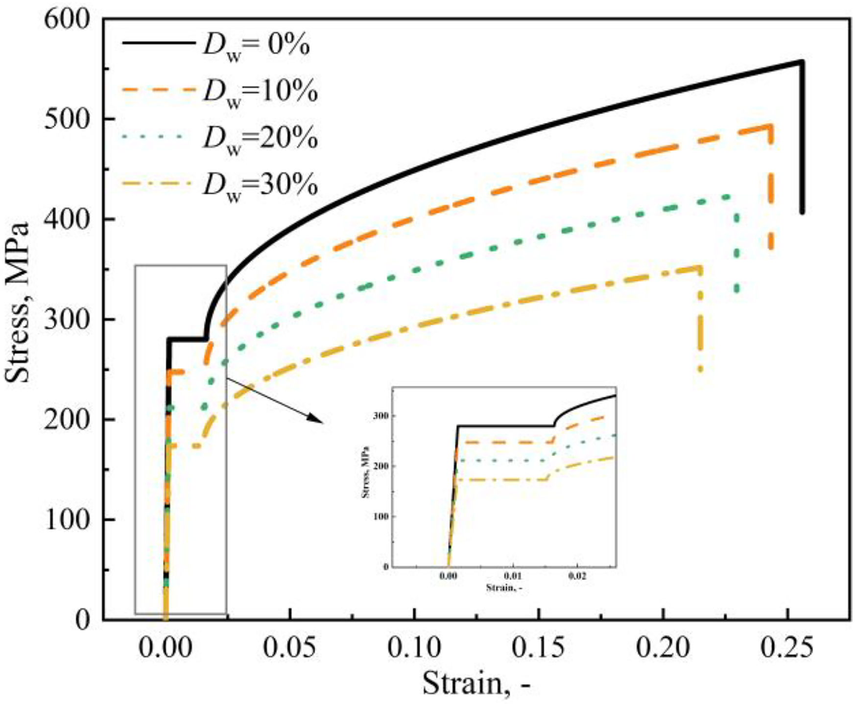
Stress–strain curves of different degradation degrees from the proposed model.

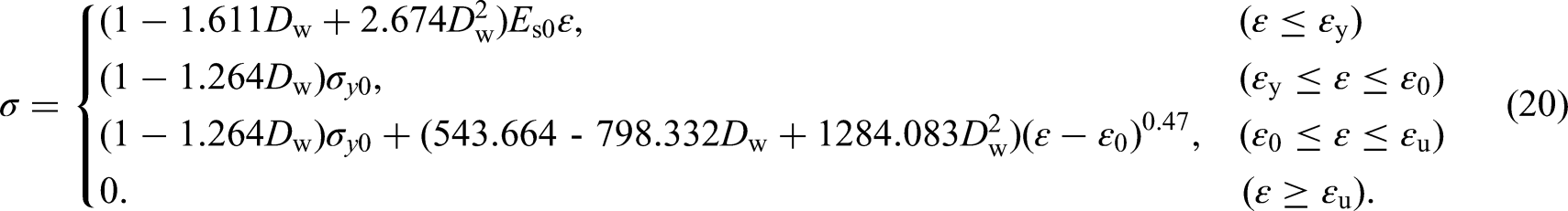
By substituting the corrosion kinetics formulation for the field exposure test (D_w= 0.015t^0.453) into equation (20), the corrosion damage constitutive model of the marine tidal zone of the Beibu Gulf with corrosion time as the variable can be obtained. Figure 18 shows the tested and predicted stress–strain curves. The predictions about the linear segments, yield strengths and ultimate strengths of the specimens are close to the test data. Although the non-linear segments are slightly underestimated, the prediction errors are still rationally acceptable, which are < 5%.

Figure 18.

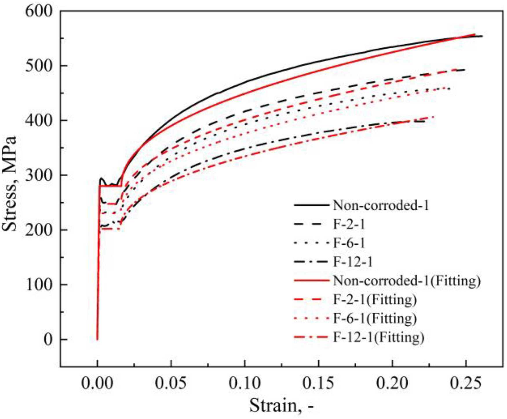
Verification of proposed model with test results.

This type of stress–strain curve modelling is very practical to be used in the non-linear finite element analysis of structures, subjected to corrosion deterioration and the constitutive model established here can be used as a reference for the performance assessment of steel structures affected by corrosion in the marine tidal zone environment.

Conclusions

To avoid failures due to corrosion and to serve as a help in marine structures safety assessment, the work presented here has studied the corrosion behaviour of CS in the tidal zone and determines the effect of corrosion degradation on specimens subjected to a tensile test. Some conclusions can be drawn as follows:

The designed simulation test can simulate the corrosion in the tidal zone. The corrosion mechanism is roughly the same and has a good acceleration effect. With the increase of corrosion degree, the mechanical properties of CS corroded under both two environments decrease similarly. However, the effect of seawater erosion on corrosion behaviour cannot be ignored.

The corrosion kinetics under both environments follow the empirical equation, D_w= Atⁿ, and the CS corrosion in the tidal environment was a deceleration process. The main reason for the higher n value of the field exposure test is that the corrosion products are washed away by the waves, resulting in a thinner rust layer.

Uniform corrosion and non-uniform corrosion are the main corrosion types of the tidal environment. Tidal corrosion can reduce the elongation of CS and even lead to brittle fracture due to non-uniform corrosion.

The diameter of corrosion pits grows over time with pits joining themselves. The corrosion pits on the CS specimens corroded under the real marine tidal zone are larger, deeper and more unevenly distributed than those under the simulation environment. The difference in the corrosion pits is the main reason for the difference in elongation of the CS with the same corrosion degree under two test environments.

A three-stage equivalent stress–strain curve of Q235B steel corroded in the real marine tidal zone as a function of the corrosion time was developed based on the regression equations and the law of the changing of parameters with different corrosion degrees was summarised. It can be used to predict the changes in mechanical properties of steel exposed to the tidal zone of Beibu Gulf at different corrosion times.