Measuring the temporal contrast sensitivity function of the phantom array effect

Abstract

The phantom array effect (PAE) has been widely investigated, but data are still insufficiently consistent to accurately predict the visibility of the PAE. One of the most critical steps towards a visibility measure is the temporal contrast threshold/sensitivity function. To determine this function, we experimentally measured the visibility threshold of the PAE at various frequencies. Participants were instructed to make 54.5° saccades in the dark across a thin light source, subtending a visual angle of 0.2° (horizontally) × 10° (vertically), with a luminance of 50 cd m⁻². Their task was to indicate in which of two sequentially presented stimuli they observed the PAE, where one stimulus was the reference driven with a direct current and one was the test stimulus, sinusoidally modulated over time. The QUEST+ method was used to change the modulation depth in the test stimulus. The results revealed a bandpass-shaped sensitivity curve of the PAE, with a peak at about 600 Hz. About 70% of the 22 participants had a peak sensitivity between a modulation depth of 0.04 and 0.13, and 65% of the 22 participants had a peak frequency between 460 Hz and 700 Hz.

1. Introduction

The nearly instantaneous response of LEDs to changing currents provokes the perception of so-called temporal light artefacts (TLAs), amongst which are flicker, the stroboscopic effect and the phantom array effect (PAE). Those TLAs are defined in the CIE 249:2022 publication ¹ written by the CIE Technical Committee 1-83 ‘Visual Aspects of Time-Modulated Lighting Systems’. More specifically, the PAE is defined as the change in perceived shape or spatial layout of objects, induced by a light stimulus whose luminance or spectral distribution fluctuates with time, for a non-static observer in a static environment. Models that predict the visibility of flicker (i.e. FVM, the flicker visibility measure, and $P_{\mathrm{st}}^{\mathrm{LM}}$ , where ‘st’ stands for short-term and ‘LM’ indicates that it is a measure quantifying the luminance waveform) and the visibility of the stroboscopic effect (i.e. SVM, the stroboscopic visibility measure) are described in the literature^1–4 and have been widely applied since then. For the PAE, however, no standardized model that predicts the visibility threshold is available yet.

Research on the PAE started before the wide use of LEDs. The focus of those earlier studies^5–10 was to understand the process of eye movements (i.e. saccades) using flashed light sources. Though fundamental and interesting in itself, the outcome of these studies does not enable us to build a model that quantifies the visibility threshold of the PAE in various LED applications.

What these studies already do tell us is that the PAE is most easily observed in low-light situations; in practice, people typically observe the artefact when driving at night behind a vehicle with LED-based (and usually, time modulated) rear lights or in indoor and outdoor luminaires (and displays) using PWM dimming at low illuminance levels. ¹¹ Therefore, most experimental investigations on this TLA have been conducted with bright light sources in a dark room (i.e. room illuminance <1 lx, measured at the eye of the observer). Some of these studies have focused on measuring the visibility of the PAE, while others have asked observers to rate its noticeability and annoyance.^12,13 Since our long-term goal is to build a model that predicts the visibility threshold of the PAE, we here focus on the visibility-related studies.

A detailed literature review on the PAE was given in CIE 249:2022. ¹ It reported psychophysical studies, in which various variables were examined, including (1) individual characteristics, such as age, gender and saccade speed;^14,15 (2) characteristics of the light modulation, such as time-averaged luminance, ¹⁶ temporal frequency,^14,17–19 modulation depth, waveform shape,^11,17,20 duty cycle and chromaticity^16,17,21,22 of the light source; and (3) characteristics of the viewing geometry like foveal or peripheral view, light source size ¹⁶ and distribution, saccade amplitude ¹⁴ and relative motion of the light source to the observer. ²³

Some of these studies have shown that the PAE is visible at temporal frequencies up to 15 kHz, as discussed in Brown et al., ²⁴ Roberts and Wilkins ²⁵ and Kang et al. ²⁶ Other studies, for example, Wang et al. ¹⁴ stated that on average people cannot perceive the PAE at frequencies close to or above 3000 Hz. Though it is important to explore what the maximum frequency is when the PAE is still visible (i.e. similar to the critical fusion frequency, CFF, for flicker), here we are mainly interested in investigating the shape of the sensitivity curve, including its peak and symmetry.

More recently, and with the aim to determine a visibility metric, Miller et al. ²⁰ explored the visibility of the PAE by using an integer rating scale (i.e. from 0, which means no pattern visible, to 6, which means highly visible repeating pattern) and checked how well SVM could predict the visibility of the PAE. The conclusion is that a separate metric is needed since SVM only exhibited a very weak correlation with the visibility of the PAE. As a follow-up on this exploration, Tan et al. ²⁷ proposed the first measure for characterizing the PAE, namely the phantom array visibility measure (PAVM) using the data collected in Miller et al., ²⁰ from which the derived Minkowski exponent (i.e. used in summation of the temporal light modulation (TLM) for different frequencies) is 2.1. The approach for deriving PAVM was similar to that of SVM; however, there were differences with respect to how the visibility threshold was measured. In the development of SVM, Perz et al. ⁴ measured the visibility threshold as the modulation depth for which participants perceived the PAE in 50% of the occurrences, while for the data of Miller et al., ²⁰ it was assumed that a rating scale of 1 indicated the PAE stimulus that was just visible. More specifically, stimuli for which 50% of the 36 participants gave a rating of 1 or larger were considered as ‘just visible’. How well the visibility thresholds in this definition describe the sensitivity function (also in line with earlier studies) needs validation.

Though the CIE ¹ pointed out that further studies are needed to determine the full temporal contrast threshold function, they nonetheless provided an example of the temporal contrast threshold function for the PAE, as shown in Equation (1):

$$T_V(f)=75.06·\exp (-0.004f)+6.86·\exp (0.001f)$$

(1)

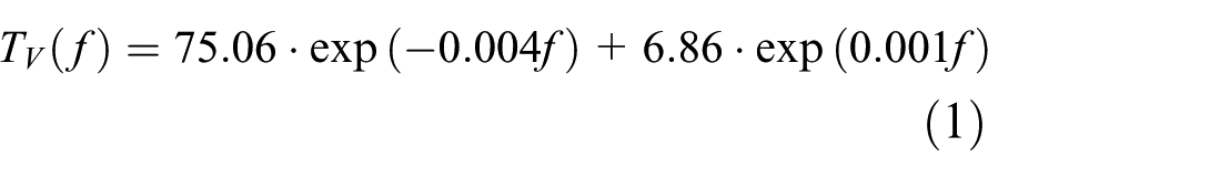
where f is the temporal frequency in Hz and T_V refers to the threshold visibility. From this equation, it can be derived that the peak sensitivity is around 755 Hz. Yu et al. ¹⁷ attempted to model their visibility threshold data using the spatial contrast sensitivity function (CSF) proposed by Barten. ²⁸ However, using this model resulted in a higher peak sensitivity (at 1000 Hz) than what was experimentally measured (with a peak at 600 Hz). The model given by the CIE (in CIE 249:2022) ¹ has a clear application context, formulated as ‘High contrast small (<2° visual angle) light sources directly visible in an otherwise dark environment (<1 lx) with relative movement between light source and observer, e.g. automotive lighting’. Following a similar approach (i.e. using the model of Barten), a provisional model of the sensitivity function of the PAE for a point light source was suggested by the CIE, ¹ in which Barten’s model ²⁸ was used for theoretical computations. However, no equations were given for this provisional model.

Kong et al. ²² adopted a third-order polynomial fit (Equation (2)) to model the sensitivity of the PAE for red, green and warm white light; this, however, is just a curve fit without any input of the underlying visual processing mechanism of observing the PAE.

$$S_{{\log }_{10}}(f_{{\log }_{10}})=\sum _{i=0}^3{p}_i{f}_{{\log }_{10}}^i$$

(2)

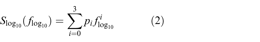
where f_log10 is the base-10 logarithm of the temporal frequency and S_log10 is the log₁₀-transformed sensitivity to the PAE. According to the dataset, ²⁹ the peak frequencies using Equation (2) for the red, green and warm white light were 580 Hz, 620 Hz and 500 Hz, respectively.

Note that to maintain clarity in notation following Equation (2), we define S as the sensitivity to the PAE and f as the temporal frequency in Hz. When a base-10 logarithmic transformation is applied, we denote the transformed sensitivity as S_log10 and the transformed frequency as f_log10. This notation is used consistently throughout the paper to distinguish between raw and transformed quantities and to avoid ambiguity in equations and figures. Alternatively, when referring to the transformation explicitly as a function, we use log₁₀(S) and log₁₀(f), respectively.

The most recent sensitivity function, proposed by Tan et al., ²⁷ is given in Equation (3):

$$S(f)=\frac{5679}{f}·\exp (-\frac{{(\ln f-7.987)}^2}{2.885})$$

(3)

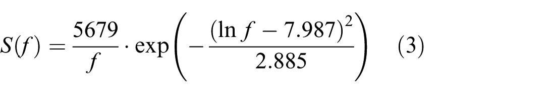
where f is the temporal frequency and S is the sensitivity to the PAE. Tan et al. ²⁷ also emphasized that a proper interpretation of PAVM values is critical to its implementation, as those values are ‘tied to the experimental conditions that underlie the measures, including source size, luminance contrast of the target against its background, relative movement and saccade speed’.

To validate the temporal contrast sensitivity functions (TCSFs) of the PAE, we performed an experiment to collect visibility threshold data as a function of temporal frequency with 10 values between 80 Hz and 1800 Hz, which is where the peak sensitivity is likely to lie.

2. Method

The experiment was designed to measure the visibility threshold of the PAE at various temporal frequencies. To do so, a two-interval forced-choice (2IFC) task was used. More particularly, participants were instructed to view two sequentially presented stimuli (i.e. a reference stimulus that was driven with a direct current (DC), and a test stimulus that was temporally modulated with a sinusoidal waveform) and indicate in which of the two stimuli the PAE was observed. A Bayesian adaptive psychophysical procedure named QUEST+, ³⁰ implemented as a MATLAB toolbox ³¹ was used to change the modulation depth of the sinusoidal waveform in the next stimuli pair based on the participant’s previous response(s). The resulting data were fitted to determine the visibility threshold (expressed as modulation depth varying between 0 (i.e. DC light) and 1). Details of the experimental setup, stimuli, method and analysis are given below.

2.1 Experimental setup

The experimental setup is shown in Figure 1. The light source was a customized luminaire that was described elsewhere. ³ It consisted of eight rows of high-power LEDs: four rows of Lumileds LUXEON Rebel (6500 K, not used in the current experiment; Lumileds Holding B.V., Schiphol, the Netherlands), and four rows of Lumileds LUXEON Rebel (2700 K). A customized diffusor consisting of multiple layers of coloured filters (Lee 216 White Diffusion; LEE Filters, Andover, Hampshire, UK) was placed in front of the LEDs to make the light output spatially more uniform. A luminance non-uniformity of 14% was measured vertically using a manufacturer-calibrated spectroradiometer (JETI Specbos 1201; JETI Technische Instrumente GmbH, Jena, Germany).

Figure 1

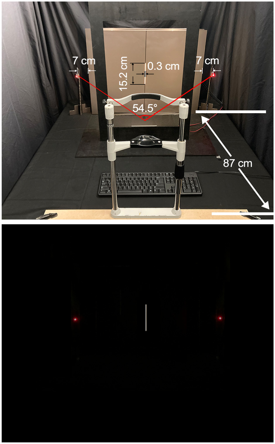
Experimental setup with ambient light ON and OFF

A programmable waveform generator (Agilent 33522B Series; Keysight Technologies Inc., Santa Rosa, CA, USA) was used to control the light output (i.e. temporal frequency and modulation depth) via TCP/IP protocol on a laptop running MATLAB R2021a (The MathWorks, Inc., Natick, MA, USA). An electronic load (Agilent N3300A; Keysight Technologies Inc., Santa Rosa, CA, USA) was used to drive the LEDs with a linear current-to-voltage curve. The TLM luminaire was placed behind a thin vertical slit made from black foam boards. The slit was sized 0.3 cm × 15.2 cm, which subtended a visual angle of 0.2° (horizontally) × 10° (vertically) when being viewed by the participants at a distance of 87 cm.

To limit head movements of the participants, a chin rest was placed in front of the TLM light source at a distance of 87 cm. To facilitate the participants with making saccades across the TLM light source, a red LED, driven by batteries, was placed at each side (horizontally) from the TLM light source, spanning an angle of 54.5°.

Measurements of the TLM light source with a spectroradiometer (the JETI Specbos 1201) showed that the TLM light source with diffusers could reach a maximum luminance exceeding 20 000 cd m⁻². The relative spectral power distribution (SPD) of the TLM light source for nine different constant driving voltages, spread over a substantial range of luminance values (i.e. 60 cd m⁻² to 1200 cd m⁻², and at each value averaged over three repetitions) is shown in Figure 2. Only for the lowest driving voltage, there is a somewhat larger deviation of the average relative SPD. Those differences, however, did not lead to perceptual differences during the experiment. The SPDs and their corresponding CIE x, y coordinates, as well as calculations of the colorimetric differences, are provided in Supplemental Tables S1 and S2.

Figure 2

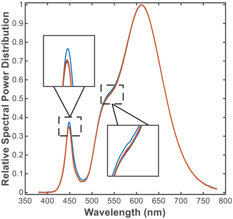
The relative SPD of the TLM light source, averaged over three repetitions for each of the nine different driving voltages (shown in a different colour). The average relative SPD which deviated the most from the rest came from the lowest driving voltage (i.e. the blue curve, corresponding to a time-averaged luminance value of 60 cd m⁻²)

Since using a high luminance in a dark environment is very uncomfortable for the participants, we decided to use a (time-averaged) luminance of the TLM light source of 50 cd m⁻² (proven to be an acceptable luminance value in an earlier study). ²² However, only a very small input voltage (i.e. less than 20 mV peak-to-peak) was needed to realize this luminance level, which implied that generating waveforms with a small modulation depth (i.e. less than 0.05) would cause quantization errors due to the voltage resolution of the waveform generator. To solve this issue, a larger voltage was used, but the luminance of the TLM light source was reduced by putting a piece of grey paper as a neutral density filter in front of the diffusor. Its transmittance fluctuated between 15% and 20% in the visible spectral range.

The TLM light source (with the grey paper) was then calibrated (again with the same spectroradiometer) at the following six driving voltages: 20 mV, 60 mV, 100 mV, 140 mV, 180 mV and 220 mV peak-to-peak. Each driving voltage was measured three times, resulting in 18 measured luminance values. Those three repeated measurements were averaged, and the relation between voltage and luminance was plotted in Figure 3. An almost perfect linear relationship (i.e. R ²  = 1) was found. The CIE x, y coordinates of the TLM light source with grey paper were x = 0.4725 and y = 0.4148.

Figure 3

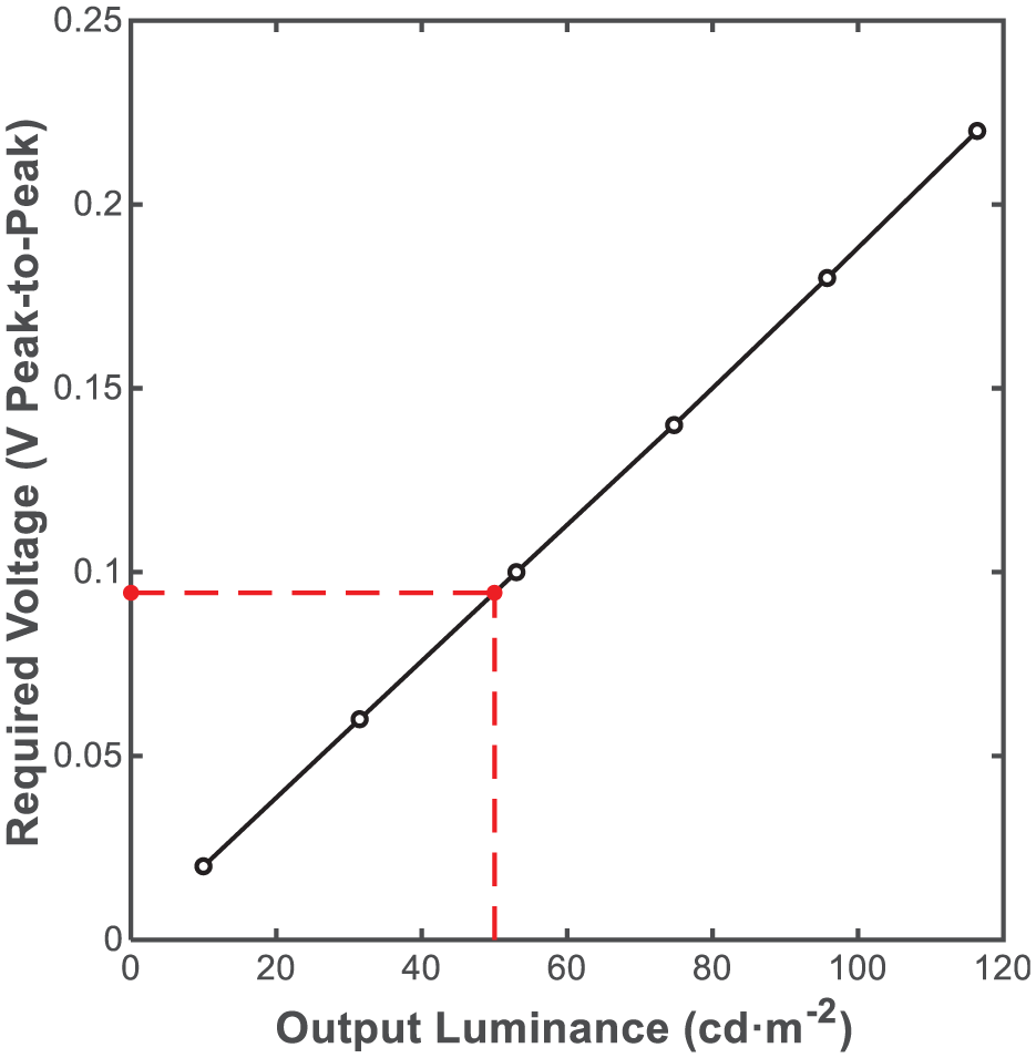
The relation between driving voltage and output luminance for the TLM light source with a grey paper in front of it. The open circles represent the measured luminance values at the six driving voltages, while the solid circle and dashed line represent the computed required voltage of 94.4 mV (0.0944 V) peak-to-peak for a target luminance of 50 cd m⁻²

2.2 Stimuli

To measure the visibility threshold of the PAE as a function of temporal frequency, sinusoidal waveforms (in luminance) were generated at 10 frequencies: 80 Hz, 160 Hz, 200 Hz, 300 Hz, 400 Hz, 600 Hz, 900 Hz, 1000 Hz, 1200 Hz and 1800 Hz. These frequency values were distributed over a range for which the PAE was expected to be visible.^12,17–19 The waveforms were characterized by their modulation depth (M), defined as the Michelson contrast:

$$M=\frac{L_{v,max}-L_{v,min}}{L_{v,max}+L_{v,min}}$$

(4)

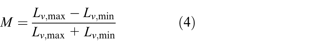
with L_v,max and L_v,min being the maximum and minimum luminance in the waveform, respectively. Analysis of the waveform generator data verified that the waveforms consistently retained their sinusoidal form across all modulation depths, with any deviations being negligible and having no meaningful impact on the results.

All stimuli were presented as pairs shown sequentially with one stimulus being the reference (DC driven with the same luminance as the (time-averaged) luminance of the test stimulus) and the other one being the (temporally modulated) test stimulus. Whether the reference or test stimulus was shown first was randomized, but with the constraint that the reference was shown first for half of all pairs (counterbalanced design).

As prescribed in Watson, ³⁰ the modulation depth (other than zero, which means a DC-driven stimulus) as expressed in Equation (4) needs to be transformed to a logarithm scale (i.e. in dB) for its use in the QUEST+ method; hence, we used:

$$s_i=20·{\log }_{10}{M}_{\mathrm{i}}$$

(5)

with M_i representing the ith stimulus in the linear space (so, the M as defined in Equation (4)), and s_i representing the ith stimulus in dB.

2.3 Experimental conditions

A full within-subject design was adopted, in which all participants were presented with 10 frequencies. Based on the results of a pilot experiment, we decided to stop the QUEST+ algorithm after a fixed number of 30 stimuli pairs, resulting in 300 (i.e. 10 frequencies × 30 trials) 2IFC-comparisons for each participant. The stimuli with a time-averaged luminance of 50 cd m⁻² were shown in a dark room with a background illuminance (i.e. the vertical illuminance measured at the foam board) of less than 1 lx and a vertical illuminance measured at the eyes of less than 1 lx (both measured with the JETI Specbos 1201).

2.4 Procedure

The experimental protocol was approved by the Ethical Review Board at Eindhoven University of Technology. All participants were recruited either from the university’s participant database or from the experimenters’ network. The selection criteria were a visual acuity higher than 0.65 (measured with the Landolt C test at 5 m distance), aged between 18 years and 45 years and no history of light sensitivity, migraine or epilepsy. The detailed procedure described below is also illustrated with a timeline in Figure 4.

Figure 4

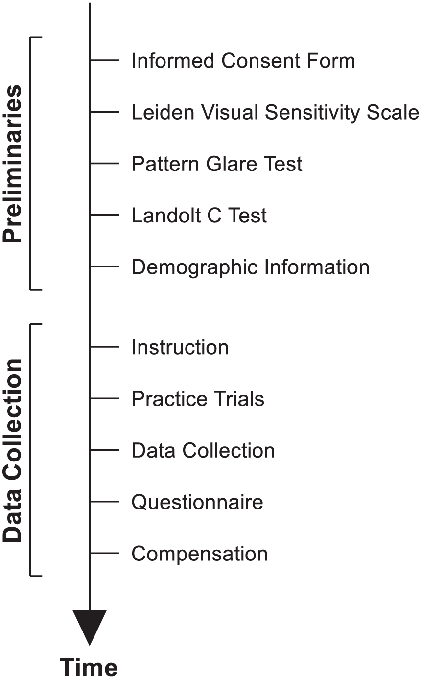
Timeline of the experimental procedure

The participants were welcomed in the lab by the experimenters. They were asked to first read and sign the informed consent form. Their sensitivity to light and contrast was measured with the Leiden Visual Sensitivity Scale (LVSS), ³² which consists of 10 rating questions. Secondly, the Pattern Glare Test (PGT) ³³ was carried out with patterns of three spatial frequencies (i.e. 0.1 cycles per degree (cpd), 3 cpd and 12 cpd). Those tests were used to exclude very sensitive participants who would be likely to experience negative effects (e.g. headaches, malaise and blurred vision) during the experiment. Thirdly, the Landolt C test was administered, to confirm that participants had a (corrected) visual acuity higher than 0.65. Then, demographic information (including age, gender and lens or prescription glasses information (if any)) was collected. Specifically, participants were also asked about their general knowledge of light and lighting, as well as whether they had experience with participating in light and lighting experiments.

They were then instructed to sit in a chair, the height of which could be adjusted, such that the eyes were at the centre of the slit. The participants were first shown images of the PAE on a computer screen, so that they understood what they were about to see. Then the lights in the experiment room were turned off, so that the participants could start adapting to the experimental condition. During this adaptation period, we gave the participants oral instructions on how to look at the stimuli and give their input. A constant light source was presented, and the participants were instructed to make saccades from one red LED light on one side of the slit to the red LED light on the other side of the slit. The saccade direction did not matter, as long as they made several rapid horizontal saccades between the two red LEDs. Afterwards, a modulated light at 600 Hz with a modulation depth of 0.95 was presented, and the participants were instructed to make saccades again. Based on the results of a pilot experiment, all participants were expected to see the PAE for this stimulus clearly.

The participants were facilitated with audio cues, that is, computer-generated voice instructions as ‘First stimulus’; ‘Second stimulus’; ‘Input recorded’; ‘Invalid input, please input again’. After hearing ‘First stimulus’, the participant was asked to make several saccades. Four seconds later, the instruction ‘Second stimulus’ was given, and the participant had to make several saccades again. After having seen both stimuli, they were instructed to use the left arrow key to indicate that the PAE was observed during the first stimulus, and the right arrow key to indicate that the PAE was observed during the second stimulus. Specifically, they were told that the PAE could be observed in only one of them, and they were allowed to guess when they did not see the PAE at all. A post-experiment analysis showed that the duration of the first stimulus (based on 220 entries, i.e. = 22 participants × 10 frequencies) was on average of 4.3 s (±0.01 s). The duration of the second stimulus was variable as it was ended with a response of the participant; this resulted in an average value of 4.9 s (±2.1 s). The average duration of both stimuli for the 22 participants at 10 frequencies is provided in Supplemental Tables S6 and S7, and Supplemental Figure S3.

Subsequently, several practice trials were given to the participants to familiarize them with the experimental task before the actual start of the experiment. The practice trials consisted of first an easy part and then a more difficult part. The easy part consisted of four pairs of stimuli, in which the test stimulus in each pair was a sinusoidal waveform at 600 Hz with a modulation depth of 0.95. We expected the right answer all four times when indicating the stimulus with the PAE in the pair. Subsequently, the more difficult part consisted of four pairs of stimuli, in which the test stimulus in each pair was modulated at 600 Hz with a modulation depth of 0.05. After these practice trials, the participants were invited to ask remaining questions, which were answered by the experimenters before the actual start of the experiment. The whole practice time lasted at least 5 min, and hence was long enough to consider the participants adapted to the dark environment.

Finally, the actual data collection started. The red LEDs (in Figure 1) were turned off (in order to avoid disturbance), and the participants were asked to make saccades with roughly the same amplitude as during the trials. The collected data consisted of 30 pairs of stimuli (the modulation depth of which was determined with the QUEST+ method) for 10 different frequencies. The resulting 300 pairs of stimuli were not grouped by frequency, but all intermingled, in an order also blind to the experimenters. When finished, the participants would hear ‘Congratulations! You finished the experiment. Thank you for your participation’. Then the lights in the room were turned on, and the participants were asked to fill in a questionnaire (given at the end of the Supplemental Material). Since the experiment was tiring, the participants were allowed to take breaks whenever necessary during the experiment, but they had to remain seated.

2.5 Participants

Twenty-three participants (9 male and 14 female), aged between 24 years old and 43 years old (29.8 ± 4.5), signed up for the experiment. No participant was excluded based on the LVSS and PGT. One participant quitted the experiment after the practice trials because he/she could not see the PAE at all during the practice trials. Thus, in the end, the data for both sessions were collected for 22 participants. The participants spent between 42 min and 67 min (53.3 ± 6.8) in the laboratory to finish the 300 trials. The time spent by each participant is provided in Supplemental Table S8.

3. Results

3.1 Calculation of the visibility thresholds

The data collected in the experiment can be plotted in a graph of the percentage of correct responses as a function of modulation depth, per frequency and per participant. Through the data in each graph, a so-called psychometric function can be fitted. We chose the Weibull cumulative distribution function as the psychometric function to fit our data and used the maximum likelihood method provided by the MATLAB toolbox ³¹ to perform the fitting. The Weibull cumulative distribution function ³⁰ has the following general form of Equation (6):

$$q=1-\lambda +(\gamma +\lambda -1)·\exp (-10^{\frac{\beta ·(s-\alpha )}{20}})$$

(6)

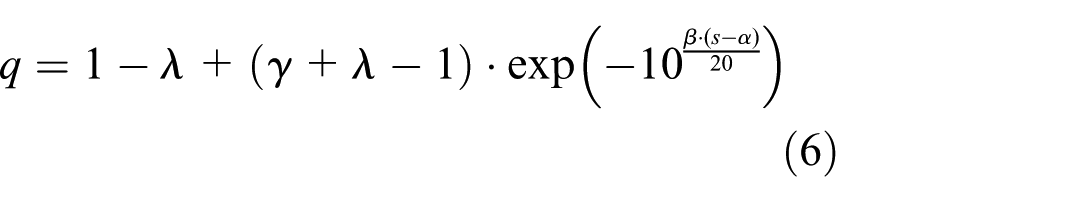
where q is the proportion (between 0 and 1) of correct responses; s is the stimulus intensity (i.e. in our case, the modulation depth, in dB, computed using Equation (5)); γ is 0.5 (i.e. assuming a 50% chance for a correct response when a participant guesses in a 2IFC task); λ is 0.02 (i.e. assuming a 2% chance for a participant to press the wrong key); β is the slope of the psychometric function (which we fixed in our fitting to 3); α is the estimated threshold in dB.

The visibility threshold is defined by the 0.75 (i.e. the mid-point between the guessing probability of 0.5 and the certainty level of 1) correct responses point on the psychometric curve. The psychometric functions for all the participants and frequencies are shown in Figure 5.

Figure 5

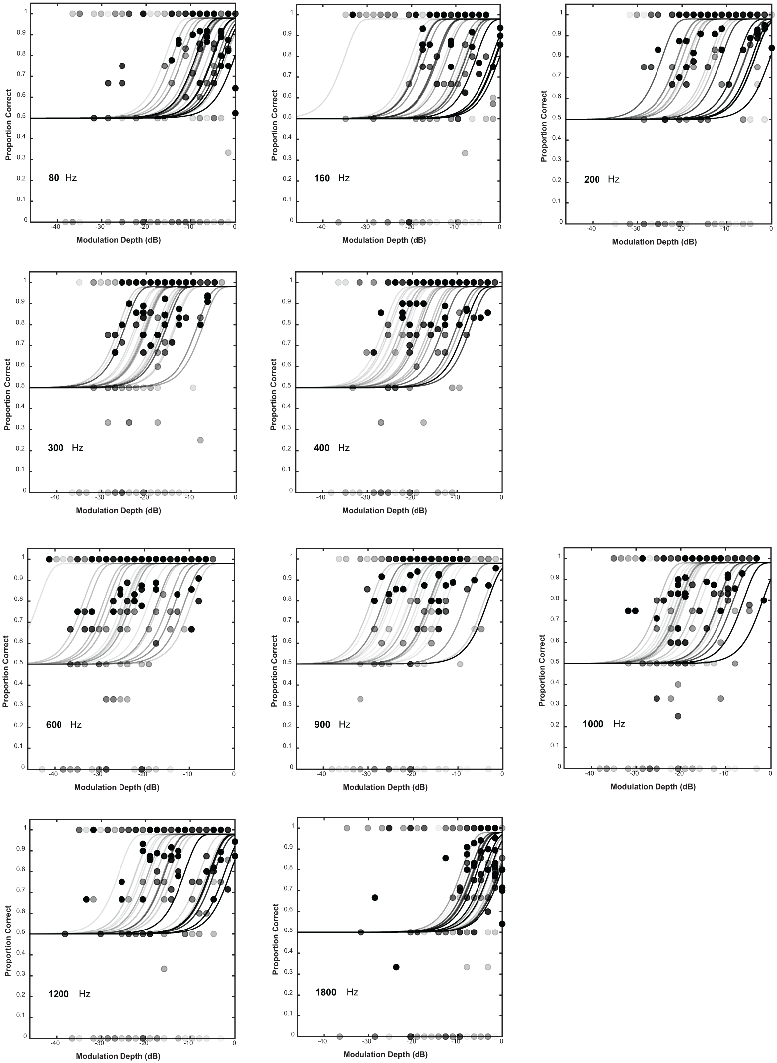
The psychometric functions, with the y-axis representing the proportion of correct responses and the x-axis representing the modulation depth in dB, for all the participants (collected in one graph) per frequency

Since we basically are interested in the visibility threshold, and hence in the 0.75 correct responses point on the psychometric curve, the exact value of slope in Equation (6) is not very relevant here, unless it strongly impacts the modulation depth corresponding to the 0.75 correct responses point. To check the latter, we compared the results of the fit in terms of modulation depth threshold for a fixed slope (= 3) versus a variable slope (i.e. between 1 and 5). Ninety percent of the visibility thresholds had a difference smaller than 10%, while the average difference was 5.5%. Thus, since the use of a fixed or variable slope in the fit of Equation (6) yielded very comparable results, we decided to continue with one approach, being a fixed slope.

The sensitivity is often defined as the reciprocal of the visibility threshold in linear space. Thus, the sensitivity to the PAE is expressed as follows:

$$S={10}^{-\alpha /20}$$

(7)

where S is the sensitivity to the PAE, and α is the estimated threshold in dB, using Equation (6).

3.2 Effect of temporal frequency on the visibility of the PAE

Through the fitting procedure described above, 220 thresholds (= 22 participants × 10 frequencies) were determined and transformed into sensitivities. The resulting sensitivity as a function of frequency, averaged over all 22 participants, is given in Figure 6, with the error bars representing the 95% confidence interval (CI) around the mean. The sensitivity clearly is higher at the medium frequencies, with the maximum at 600 Hz (with a mean M threshold of 0.07), and the sensitivities are substantially lower at the two far ends of the measured frequency range. The mean M thresholds for 80 Hz and 1800 Hz are 0.45 and 0.65 respectively.

Figure 6

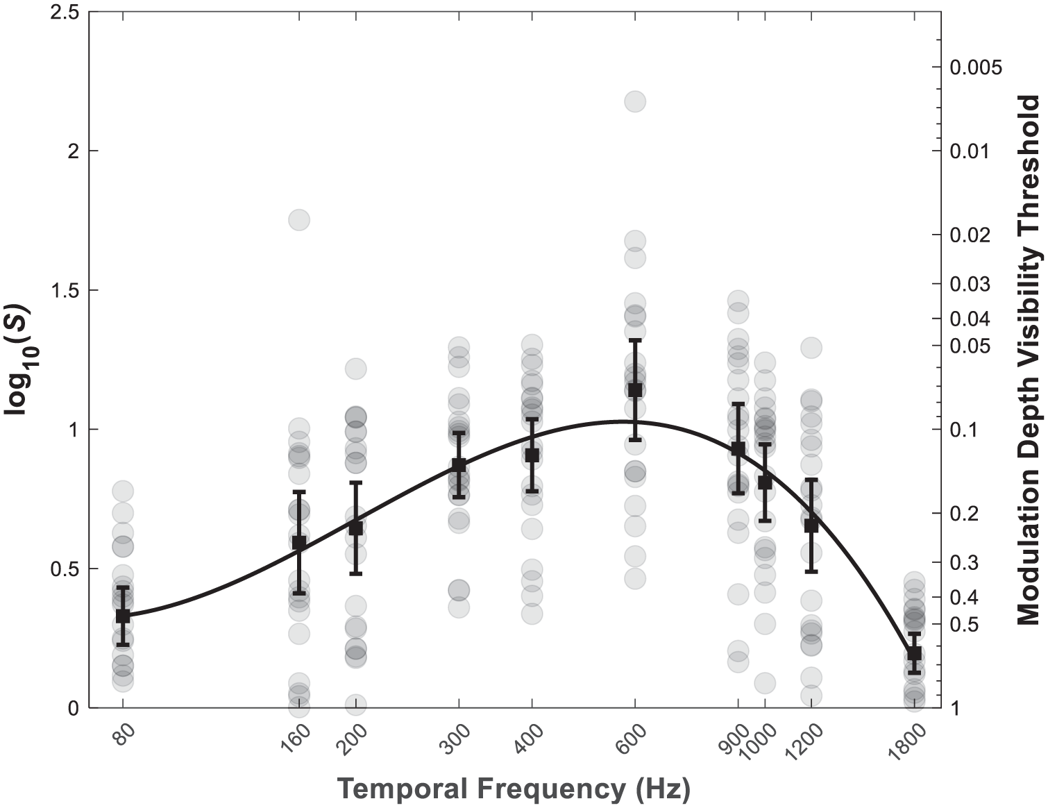
Visibility threshold expressed as log₁₀(S) (left y-scale) and modulation depth threshold (right logarithmic y-scale) as a function of frequency (in logarithmic scale), averaged over the 22 participants. The error bars represent the 95% CIs of the mean. The symbols represent individual sensitivity data points

The black line through the mean sensitivity values is a third-order polynomial fit, according to Equation (2). The parameters of the polynomial fit are 20.6292 (p₀), −28.3286 (p₁), 12.8125 (p₂) and −1.8557 (p₃), respectively. The chi-square value for the fit is 0.220, indicating that the fit passes the criterion for goodness of fit at the 0.05 significance level.

In order to test the overall effect of Frequency on the visibility of the PAE, a linear mixed model (LMM) analysis was performed using IBM SPSS Statistics (Version 28; IBM Corp., Armonk, NY, USA), with logarithmic transformed sensitivity values (S_log10) as the dependent variable, and logarithmic transformed temporal frequency (f_log10) as the fixed independent variable. A random intercept for Participant was also included. The results of the LMM analysis show a significant effect of Frequency (F(9, 198) = 33.187, p < 0.001). In addition, there is a significant effect of intercept (F(1, 22) = 209.723, p < 0.001), which implies substantial individual differences.

3.3 Effect of Participant on the visibility of the PAE

The statistical results showed significant individual differences in their sensitivities to the PAE. Equation (2) was applied to each of the participants individually, and the results are shown in Figure 7. For most of the participants, bandpass-shaped curves were obtained, though for some participants, the data were noisy (e.g. Participant 05).

Figure 7

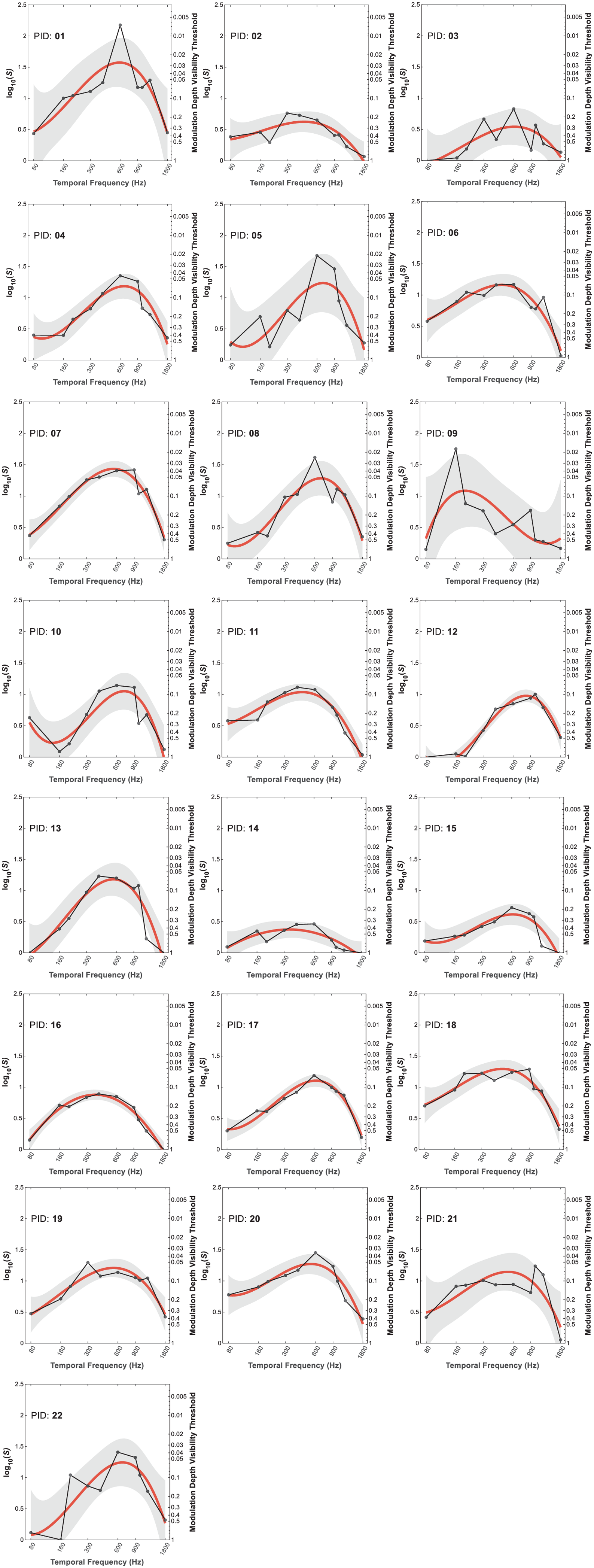
Visibility threshold expressed as log₁₀(S) (left y-scale) and modulation depth threshold (right logarithmic y-scale) as a function of frequency (in logarithmic scale) per participant. The symbols represent individual sensitivity data points. The lines represent the third-order polynomial fits, while the shaded areas indicate the 95% CIs of the fits

For each of the third-order polynomial fits, the peak frequency and peak sensitivity were obtained; they are shown in Figure 8. The dashed lines represent the mean peak sensitivity (S_log10 = 1.07, corresponding to an M of 0.085) and the mean peak frequency (i.e. about 550 Hz), respectively. About 70% of the participants (i.e. 15 out of 22) had a peak sensitivity between a modulation depth of 0.04 and 0.13, and 65% of the participants (i.e. 14 out of 22) had a peak frequency between 460 Hz and 700 Hz. The peak sensitivities ranged from 0.37 (i.e. an M of 0.42) to 1.57 (i.e. an M of 0.027), with a standard deviation of an M of 0.098. The peak frequencies ranged from 200 Hz to 810 Hz, with a standard deviation of 140 Hz. However, it is worth noting that the peak frequency of 200 Hz for Participant 09 is probably a consequence of an outlier, as can be visually inspected in Figure 7.

Figure 8

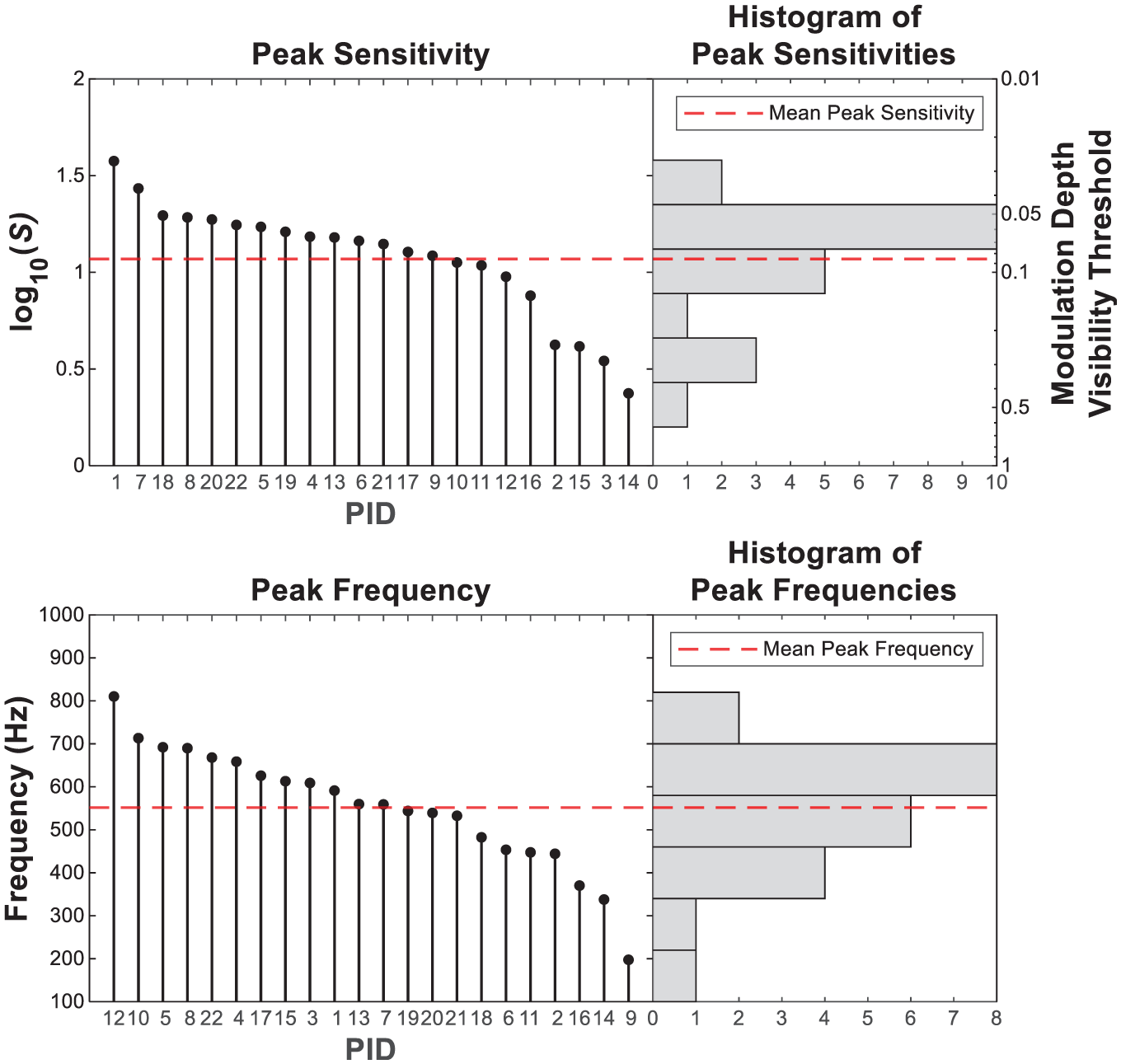
The sorted peak sensitivities expressed as log₁₀(S) and peak frequencies ordered by Participant ID (PID) and the histograms of peak sensitivities and peak frequencies from the individual third-order polynomial fits. The individual peak sensitivity and peak frequency are provided in Supplemental Table S9

3.4 Questionnaire analysis

The answers to the questions we asked at the end of the experiment are summarized in Figure 9. Question 1 was an open question asking ‘How do you feel now?’ Almost all participants indicated tired or dry eyes because constantly making saccades is not common in daily life. According to Proudlock and Gottlob, ³⁴ the head of the observer can be still when making a horizontal saccade within approximately ±50° (i.e. the normal human oculomotor range). However, there is a tendency to make head movements in response to horizontal saccades outside of the range of ±10°. In our experiment, the requested saccade amplitude was about ±27°, which indicates that the participants might have had to make extra efforts to avoid head movements. About 73% of the participants (i.e. 16 out of 22) found the task sometimes difficult, which could be expected when using an adaptive procedure. The majority of the participants (i.e. 17 out of 22) were somewhat or fairly confident about their responses during the experiment. In addition, 3 out of 22 participants mentioned that they would have liked the option to indicate that they were ‘not sure’ during the experiment. During the debriefing, participants were explained why a 2IFC task was chosen.

Figure 9

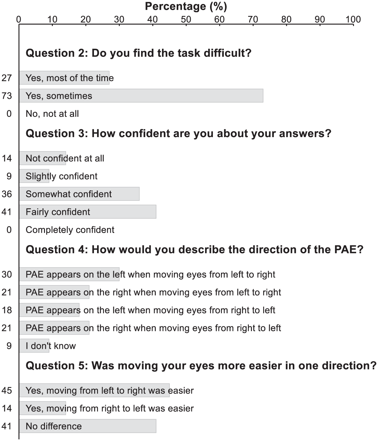
Summary of participant responses to the post-experiment questionnaire (Questions 2–5). For each question, the numerical values to the left of the response options indicate the percentage of participants selecting that option. These percentages are also represented by the length of the horizontal shaded bars, aligned with the top axis labeled “Percentage (%)”

Question 4 (‘How would you describe the direction of the PAE?’) was difficult for the participants as they were not instructed to pay attention to the direction of the PAE at the start of the experiment; they thus could only recall their memories. In addition, we intentionally did not control for the direction of the saccade, so the participants could use their own preferred direction for making a fast movement of their eyes. As a consequence, they probably did not see the PAE in a constant direction across the experiment. More than half of the participants (i.e. 13 out of 22) responded that there was a difference between moving their eyes in different directions. As such, our results on Question 4 do not really align with the study of Hershberger and Jordan, ⁶ in which 53 of the 58 observers perceived the PAE in the opposite direction of the saccade. But since question 4 was just meant to be exploratory in this study, it did not affect our findings.

The results from the LVSS, PGT and the Landolt C Visual Acuity Test are given in Supplemental Table S10. To investigate the relationship of the results from LVSS, PGT and the Visual Acuity Test with the participants’ sensitivity to the PAE, we calculated Spearman’s rank correlation. Specifically, we used the individual peak frequency and peak sensitivity (i.e. expressed as S_log10) derived from the individual third-order polynomial fit to represent each participant’s sensitivity to the PAE. The Spearman correlation coefficients were 0.088 for LVSS and peak frequency (p = 0.697), 0.284 for LVSS and peak sensitivity (p = 0.200), 0.322 for PGT and peak frequency (p = 0.144), 0.467 for PGT and peak sensitivity (p = 0.028); −0.044 for visual acuity and peak frequency (p = 0.844) and −0.044 for visual acuity and peak sensitivity (p = 0.846). This shows that there is only one significant positive relationship, namely between PGT and peak sensitivity. The more sensitive individuals are to glare, the higher their sensitivity to the PAE expressed as S_log10, and so the more sensitive they are to seeing the PAE. This seems to suggest a broader increased sensitivity in the human visual system for some individuals. The PGT included three spatial patterns that corresponded to spatial frequencies of 0.1 cpd, 3 cpd and 12 cpd, respectively. For directly relating these particular spatial frequencies to the visibility of the PAE, the saccade speed is needed as discussed below.

4. Discussion

4.1 Comparing our sensitivity data with literature

As mentioned in the introduction, there exist already publications with data of visibility thresholds or sensitivities of the PAE.^14,17,22 These thresholds have been measured with different individuals, different light modulation characteristics and different characteristics of the viewing geometry, but still it is valuable to make an overall comparison of these data across literature. The data of Kong et al. ²² are available at an open-access repository. ²⁹ However, most of the raw data of these studies are not openly accessible, and therefore we used the software program PlotDigitizer: Version 3.3.9 ³⁵ to extract the data from published figures and graphs in literature. The assembled data are shown in Figure 10(a). Since we are interested in investigating both the peak and shape of the TCSF, a third-order polynomial (Equation (2)) was adopted to fit the sensitivity of the PAE wherever possible; these fits are added as dashed lines to Figure 10(a).

Figure 10

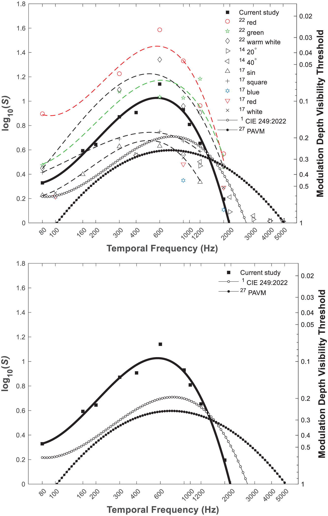
(a) The sensitivity data of the PAE reported in multiple psychophysical studies.^{1,14,17,22,27} The data points represent the mean sensitivity at a certain temporal frequency. The dashed lines represent the third-order polynomial fits. (b) Highlighting the comparison of the TCSFs between the present study, the model introduced in CIE, ¹ and the model of Tan et al. ²⁷

Figure 10(a) clearly shows that despite the sensitivity to PAE varying up to a factor of 10 in terms of absolute sensitivity, all TCSFs have a bandpass shape. It is also important to notice that the PAE visibility peaks between 400 Hz and 1000 Hz, which is in line with Miller et al. ²⁰ In addition, all the results in those studies seem to suggest that the maximum frequency where the PAE is visible is lower than 5 kHz, much lower than reported in Brown et al. ²⁴ and Kang et al. ²⁶ Actually, all these results are fairly consistent, given the reported effects of lighting and viewing conditions on the visibility of the PAE.

To highlight the comparison of the TCSF between the model (Equation (1)) introduced in CIE, ¹ our study (Equation (2)) and the model (Equation (3)) of Tan et al., ²⁷ Figure 10(a) is simplified to Figure 10(b). It is clear that both CIE ¹ and Tan et al. ²⁷ predicted a lower peak sensitivity compared to our study. The parameters for the best fit with our data using the general shape of the formula are 0.7611, 0.0071, 0.0253 and 0.0018 for Equation (1) and 7432, 6.7 and 0.9 for Equation (3).

So far, international standardization bodies such as the CIE have not recommended a specific shape for the CSF of the PAE. Literature reports a number of suggestions, but these suggestions still largely vary with the actual set of data used. The curve suggested by the CIE has a functional behaviour comparable to the one found in our study (and similar to typical spatial and temporal CSFs of human vision), and a peak sensitivity frequency comparable to our study and the one of Tan et al. ²⁷

4.2 Insights towards a general model of the TCSF of the PAE

4.2.1 Saccade speed

Since the PAE is a spatiotemporal visual phenomenon, modelling its sensitivity as a function of temporal frequency alone clearly has its limitations; expressing the sensitivity as a function of a spatially transformed variable (i.e. when the saccade speed is known) seems more appropriate. Both Yu et al. ¹⁷ and CIE ¹ attempted to utilize the spatial CSF to model the visibility thresholds of the PAE. However, translating temporal frequencies in Hz to spatial displacements in cpd requires the knowledge of the saccade speed.

Saccade speed depends on many factors, such as the type of saccade (i.e. the reactive saccade vs. the voluntary saccade), ³⁶ the saccade amplitude ³⁷ and the motivation of the observer. ³⁸ The reactive saccade is faster than the voluntary saccade ³⁶ and the observers could vary their ability to increase and decrease the velocity of their saccade when instructed to do so. ³⁸ As a general simplified function, the saccade speed is modelled as a function of the saccade amplitude (e.g. Gibaldi and Sabatini), ³⁹ and hence by fixing the saccade amplitude, we can estimate the saccade speed. The latter, however, is only true per participant, since the saccade speed is very different among individuals. As a consequence, variations in the visibility of the PAE can be partially explained by the differences in saccade speed. ¹⁵ As such, any model of the visibility of the PAE should take this into account. Future studies should therefore measure the eye saccade speed of the observers.

4.2.2 Luminance contrast

In CIE 249:2022, ¹ it was pointed out that the luminance contrast (i.e. the ratio in luminance between the temporally modulated stimulus and its background, defined as (L_s − L_b)/L_b, where L_s is the (space and time) average of the TLM stimulus luminance, and L_b is the luminance of the background, affects the visibility of TLAs. Hence, luminance contrast should be included in a general model of the PAE.

In this study, the chosen luminance of 50 cd m⁻² for the TLM light source was lower than in many real-life luminaires, such as car tail lights. However, in this experimental setup, the TLM light source was placed behind a black foam board (Figure 1) in an otherwise not illuminated room. This made the environment rather dark (i.e. the vertical illuminance <1 lx, measured at the eye of the observer as well as at the foam board), and so resulted in an L_b value close to zero. As a consequence, the luminance contrast used in the experiment was still high. The viewing distance of the participants was only 87 cm, making it a close-range task. The combination of a close-range task at high contrast made the experiment uncomfortable. As such, a pilot experiment taught us that a higher luminance of the TLM light source made the source too glary for the dark-adapted participants. In addition, due to the thin-slit geometry of the light source, a strong afterimage effect was reported, which caused confusion for distinguishing it from the PAE. For these two reasons, we have chosen to limit the luminance of the TLM light source to 50 cd m⁻². Still, to generalize our results towards a model, our data measured for a low luminance of the light source at high contrast with its environment needs to be extended to higher luminance values of TLM light source and background.

In laboratory studies, it is common to have a uniform background. However, in real-life applications, the area in the visual field around the temporally modulated light source can vary significantly in terms of spatial layout and complexity (i.e. non-uniformity), which poses another challenge to the model. To create viewing conditions that better resemble or reflect real-life conditions such as interior lighting applications and exterior lighting in the evening (including car tail lights on the roadway), more realistic luminance levels of the light source should be considered in a non-uniformly illuminated background.

4.2.3 Ambient light level

Apart from the luminance level at the background around the TLM light source, also the light level in the rest of the environment may have an effect on the visibility of the PAE, and thus should be considered for a general model of the visibility of the PAE. As mentioned in the introduction, many studies showed that the PAE is most easily observed in low-light situations. The TLM light source in Tan et al. ²⁷ had a luminance of 38 700 cd m⁻² and subtended a visual angle of 0.06° when viewed by the participants at a distance of 3 m. The total illuminance at the eye was 1.6 lx, including about 1 lx from the light source itself. As such, the PAVM (i.e. the model derived from these data) might be applicable in low-light situations, notably outdoors, such as when driving at night and observing car tail lights. However, it is unlikely to be adequate for general indoor applications with a higher illuminance since the corresponding adaptation state of the observers will influence both their temporal and spatial sensitivity (e.g. CIE 249:2022). ¹ So, to develop the visibility measure of the PAE for general lighting applications, a higher vertical illuminance at the eye than used in the literature (i.e. 1.6 lx in Tan et al. ²⁷ ; <1 lx in Kong et al. ²² ; <1 lx in Kang et al. ²⁶ ) is needed.

Also the model given in CIE 249:2022, ¹ as shown in Equation (2), has a clear application context with an otherwise dark environment (<1 lx). Under office lighting conditions, Wang et al.^18,19 showed that during normal reading (i.e. black target on white background), the PAE is generally not visible, no matter whether the illumination level is high (around 500 lx) or low (around 250 lx). Furthermore, Wang et al. ¹⁸ showed an interaction effect between frequency and illumination level on the visibility of the PAE. More specifically, the visibility thresholds were around 0.27, 0.26 and 0.275 modulation depth for 100 Hz waveforms under illumination level of 50 lx, 250 lx and 500 lx, respectively. The threshold values were around 0.4, 0.14 and 0.18 modulation depth for 600 Hz waveforms under the same illumination levels. In addition, a different ambient light level usually also influences the luminance contrast of the TLM light source indirectly, meaning that there is an interplay between those two factors, which also requires further investigation.

4.2.4 Waveforms

The sensitivity curve obtained from the conducted experiment allows to predict the visibility of the PAE for other targets and environments as long as they are similar to the experimental conditions used: that is, for sinusoidal temporal waveforms, observed with a very thin slit in high luminance contrast with the background. In the case of other waveforms, our results provide a very useful lower limit for the visibility of the phantom array. Our sensitivity curves can be applied to the relative amplitude of the dominant Fourier component of the waveform, as historically suggested by De Lange in 1954 in the case of flicker assessment based on the ‘ripple ratio’. ⁴⁰ It is useful to emphasize that any additional harmonic Fourier component present in the waveform cannot lower the visibility of the PAE, but can only increase it. A visibility measure for the PAE can be built using a formula similar to the model of the SVM. This type of formula is a Minkowski sum of the weighted harmonic components. However, the determination of the Minkowski component would require performing a new set of experiments using temporal waveforms featuring two or more harmonic components, as present in rectangular waveforms (including square wave) or even arbitrary waveforms.

The sensitivity curve also allows to predict the visibility of the PAE at other frequencies than the ones used in the current experiment, as long as they are within the range from 100 Hz to 1800 Hz. Under the current experimental conditions, the sensitivity to the PAE is already very low at 1800 Hz, and thus measuring it at higher frequencies is not so useful. Literature,^24–26 however, has shown that the PAE is still visible at frequencies beyond 1800 Hz under different experimental conditions. Hence, when changing the size of the slit and/or the luminance of the TLM light source, the background and the ambient, higher temporal frequencies should be considered to be included in the experimental design.

4.2.5 Additional parameters in the model

Apart from the most prominent aspects for modelling the PAE visibility threshold such as saccade speed and luminance contrast mentioned above, there are additional factors that affect the visibility of the PAE, and hence should be considered in an all-encompassing model. The effect of the size of the light source is discussed earlier in this paper, in relation to its effect on the brightness contrast perceived with its environment. Kong et al. ²² showed earlier that there are significant differences in the shape of the PAE sensitivity for different chromaticity of the light source. To what extent these differences can be explained by existing chromaticity differences in the spatial and temporal CSF needs further investigation.

5. Conclusion

In this study, the visibility threshold of the PAE in a dark environment (i.e. <1 lx) was measured for 22 participants. The statistical analysis revealed a significant effect of Frequency and Participant on the visibility of the PAE. With respect to Frequency, a bandpass-shaped sensitivity curve was found, with a peak at about 600 Hz corresponding to a modulation depth of 0.07. Further investigation of the effect of Participant requires the utilization of eye-tracking devices to extract individual saccade speeds. We also compared our sensitivity data with literature and found common ground for the model, despite large differences in terms of absolute values.

Despite the limitation of the experimental condition used in this study, our results provide a very useful lower limit for the visibility of the PAE. More research data on the visibility of the PAE under different conditions (i.e. different luminance levels, different luminance contrast, a broader frequency range and more waveforms) are needed to develop a robust visibility measure for the PAE.

Supplemental Material

sj-docx-1-lrt-10.1177_14771535251379686 – Supplemental material for Measuring the temporal contrast sensitivity function of the phantom array effect

Supplemental material, sj-docx-1-lrt-10.1177_14771535251379686 for Measuring the temporal contrast sensitivity function of the phantom array effect by X Kong, C Martinsons, M Nilsson Tengelin and I Heynderickx in Lighting Research & Technology

Supplemental Material

sj-xlsx-2-lrt-10.1177_14771535251379686 – Supplemental material for Measuring the temporal contrast sensitivity function of the phantom array effect

Supplemental material, sj-xlsx-2-lrt-10.1177_14771535251379686 for Measuring the temporal contrast sensitivity function of the phantom array effect by X Kong, C Martinsons, M Nilsson Tengelin and I Heynderickx in Lighting Research & Technology