
Abstract
Integrating spectral data (spectral responsivities of photometers or spectral distributions of light sources) to calculate integrated quantities such as tristimulus values is straightforward at first sight. However, estimating the measurement uncertainty of these integrated quantities is challenging. When calculating integrated photometric quantities, some uncertainty contributions from the spectral data transfer to the final results, some ‘cancel out’, some ‘average out’ and others increase or decrease their weight by correlation. The spectral data are usually assumed to be uncorrelated when deriving other quantities by integration, which is typically not justified. A method called the framework approach, applying orthogonal basis functions and Monte Carlo simulations, is introduced. This approach shows that neglecting partial spectral correlations may lead to a significant underestimation of the measurement uncertainty of integrated quantities. Furthermore, this paper shows how information about spectral error correlation structures can be used to obtain better estimations of the measurement uncertainty.
1. Introduction
Integration of spectral data is central to calculating photometric and colorimetric quantities, as well as quantities that are used to assess non-visual effects and photobiological safety. Calculating any of these quantities from spectral data involves determining the value of the measurand by numerical integrals (weighted sums) of source spectral distributions across the spectral range of the weighting functions.
This paper considers spectral integrals of the form:
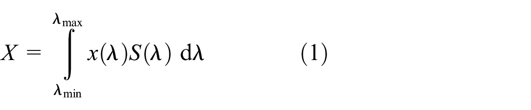
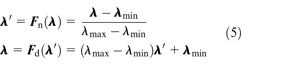
where x(λ) is a defined weighting function, S(λ) is the spectral distribution of a source or the spectral responsivity of a detector and the integral is calculated over the wavelength range λmin ≤ λ ≤ λmax. A similar spectral integral may be involved when using filtered detectors (including practical photometers). In those cases, the spectral response function, taking the place of
While these calculations are straightforward and generally calculated using a trapezium rule, estimating the associated measurement uncertainty becomes complex and challenging, as described in the CIE198-SP2 1 report. In particular, where there is a significant error correlation between measured spectral data at different wavelengths, the combined uncertainty associated with the integrated quantity is affected, as demonstrated by Schmähling et al. 2 To describe the effects that can be caused by correlations, one must first understand what ‘correlated’ means in this context. This paper also provides some assistance in this regard.
A general measurement uncertainty assessment, whether based on the law of propagation of uncertainties in the legacy GUM 3 or Monte Carlo (MC) methods introduced in the JCGM 101 4 document, starts with a measurement model written as an equation. It is common for measurement models to be multi-stage, as described in the JCGM 106 5 document. This means that some of the model’s input quantities are based on previous (earlier stage) measurement models.
For photometric and colorimetric quantities as well as quantities that are used to assess non-visual effects and photobiological safety, the measurement model will be in the form of Equation (1) and this is therefore what will be discussed in Section 2. The measurement model can be considered multi-stage in that the spectral quantity itself will be the measurand of a calibration process to determine that spectrum and will have its own measurement model.
In this work, we propagate uncertainties with complex error correlation structures through the measurement model using a method of orthogonal basis functions introduced by Kärhäet al. 6 To describe correlations, a framework approach for the estimation of dependencies is developed. This framework approach allows a better insight into the origin of those significant contributions to the measurement uncertainty of an integrated quantity, which come from correlations in the spectral distribution data.
With the framework approach, we introduce an evaluation method; its application (simply to show how it works) is presented based on an example in this paper.
The main contribution of this work is the estimation of sensitivity coefficients. Here, we use MC methods to propagate such error correlation structures, both individually – to evaluate the sensitivity of the integrated quantity to each source of uncertainty – and combined to provide a combined uncertainty for the integrated quantity. In this method, we follow the kind of sensitivity analysis proposed by the JCGM 101, Annex B, 4 which is called ‘one factor at a time’ by Razavi and Gupta. 7
Furthermore, this work considers partially correlated contributions associated with both wavelength and the spectral distribution amplitude, alongside with fully correlated and uncorrelated errors.
In spectral integrals, sources of uncertainty that lead to fully correlated errors are simple to propagate (and cancel out if the integrated quantity is normalised). Sources of uncertainty that lead to fully uncorrelated (independent) errors reduce significantly by the effective weighted averaging of the integral. Therefore, the most important sources of uncertainty are those that provide partial error correlation. In general, however, the form of that partial error correlation is unknown. For the description of partial error correlation, this paper builds on a method originally presented by Kärhäet al., 6 and extended by Vaskuri et al. 8 and Maham et al. 9 The basis function method uses a set of basis functions to model possible, (realistic) error correlation forms and uses MC methods to explore different possible correlation structures. This paper presents the final modelling equations for the basis function method and examples.
The implementation of the work presented here can be found in the open-source Python package 19nrm02, 10 which uses the LuxPy Python package by Smet. 11 Additional examples of the application of the approach, including animations in the form of mp4 files, are presented in Supplemental Material for this paper (available online).
2. Methods
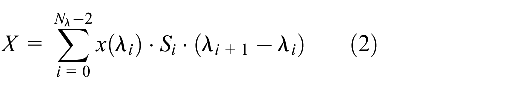
Integrals of the form of Equation (1) are treated as summations of a spectral quantity over a set of wavelengths λi:
It is useful to describe the spectral data with vector notation. In this paper, vectors are represented by bold italic symbols, and scalars are represented by thin italic symbols. For spectral data with
Amplitude vector:
Wavelength vector:
where the random values of the elements in the vectors, generated during the MC simulation (MCS), can originate from wavelength uncertainty, signal uncertainty or both. Both vectors are used to calculate the spectrally integrated quantity of interest. Initially, to better understand their individual influences, they are simulated independently.
Within this paper, where the elements of the vectors are processed individually, they are written as thin italic symbols with an index (e.g. λi) or in functional form (e.g. S(i) or S(λ)). The symbol
The elements of these two vectors are determined experimentally, and the values can be affected by three types of uncertainty that create fluctuations in them:
Effects that are uncorrelated from one element to another (random effects, noise).
Effects that are fully correlated from one element to another (systematic effects, bias).
Effects that are partially correlated, where ‘partially correlated’ can be interpreted as an infinite variety of different correlation states varying from fully uncorrelated to fully correlated.
In this paper, MCS was used to propagate uncertainties. MCS is a mathematical technique12,13 that enables a quantitative analysis of a measurement result. The core idea behind an MCS is to represent the propagation of probability density functions (PDFs) for the input quantities (here the measured values of the spectral quantity at different wavelengths) through the measurement model (here the integral given in Equation (1)).
This involves the following steps:
Random sampling: For each input quantity (here the spectral quantity at each wavelength), a set of representative errors are generated by generating random numbers drawn from the distributions.
Repeated trials: In an MCS, a large number (
Aggregation of results: After running simulations many times, the results are aggregated and analysed to estimate the statistical properties of the system being modelled, such as averages, variances, probabilities of different outcomes, correlations, etc.
2.1 Overview
A general overview of the framework approach is presented in Figure 1. The different parts of the figure will be explained in detail in this section.
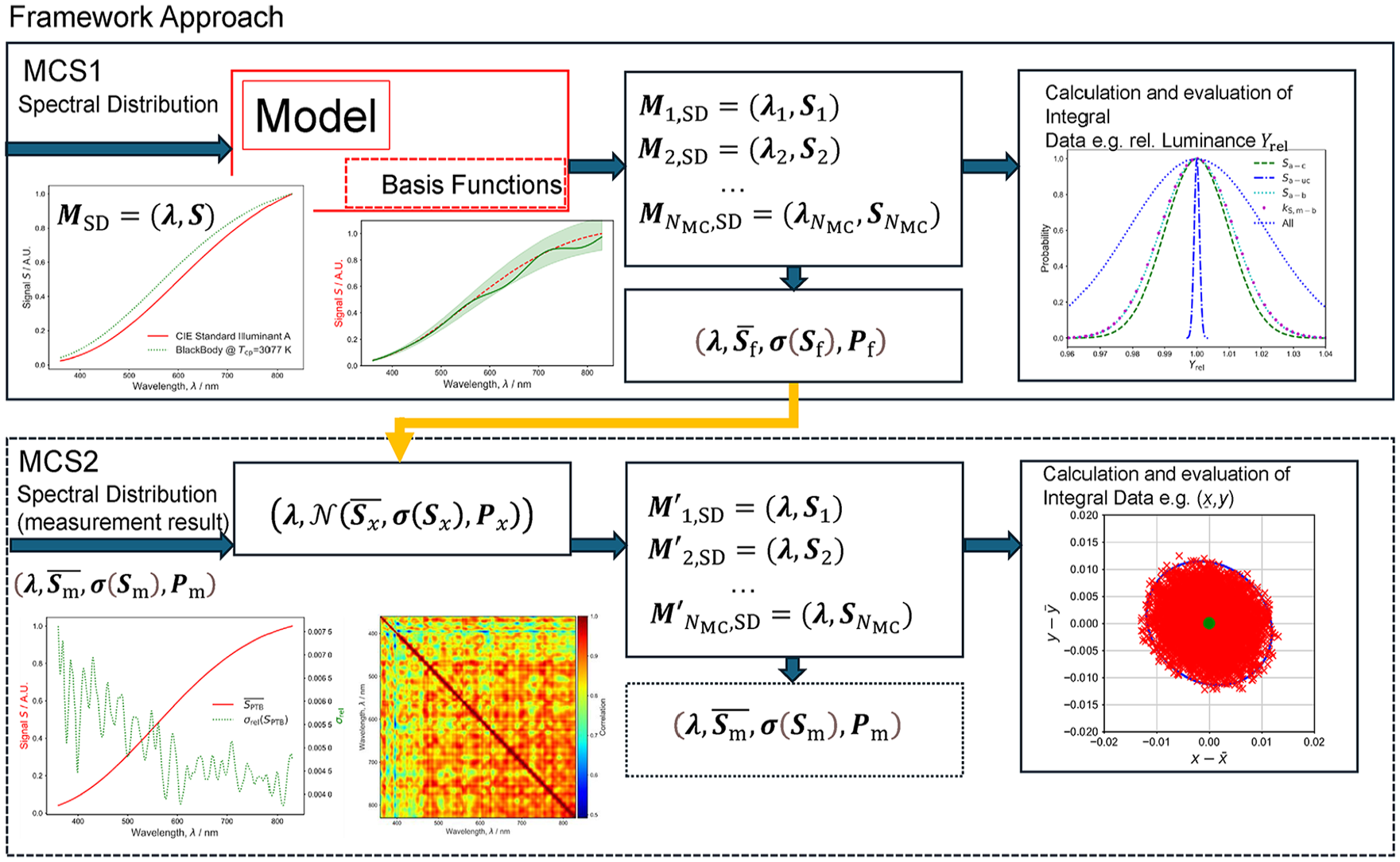
Overview of the framework approach. See Section 2.1 for definitions of the symbols used
Figure 1 shows the calculation during two separate MCSs (MCS1 and MCS2) running each
In the next step, a general model, explained in Section 2.2, uses this spectral distribution to add the measurement uncertainty by generating different fluctuations around the input spectral distribution. This is done by separately modelling the wavelength and amplitude scales with different types of simulated uncertainty contributions. The uncertainty contributions are modelled as correlated, uncorrelated and partially correlated contributions. At the end, this results in a set of
Besides the correlated and uncorrelated uncertainty contributions, generating partially correlated uncertainty contributions using the basis function technique, as described in Section 2.3, is essential for the evaluation presented here.
In this paper, the data are simulated and do not consider the physical background of a particular measurement setup or device under test to ensure that the application does not cover just one method or describe a specific measurement technique. Possible connections of the model parameter to physical models or real measurements are given in Section 2.4.
Finally, using the
Furthermore, the
In parallel to the MCS1 using the framework approach, we can use an MCS2, as shown in the lower part of Figure 1, to calculate a set of integral quantities based on a multivariate normal distribution method. This can be done using either real measurement results, for example, provided by the Physikalisch-Technische Bundesanstalt (PTB) as shown in Section 3.1 or with compressed information from MCS1 (see Section 3.2). With this method, we generate the spectral distribution data from multivariate normal distribution sampling, to again get combinations of wavelength and spectral information
2.2 Model for uncertainty contributions in the framework approach
The framework approach uses additive (subscript ‘a’) and multiplicative (subscript ‘m’) model parameters linked to the values as uncertainty components. The uncertainty contributions are implemented during the simulation as follows:
Uncorrelated (subscript ‘uc’): Every vector element represents a different realisation of a random process in each of the
Correlated (subscript ‘c’): All vector element variations behave similarly in any given MC trial. A random number is drawn for every trial only once for the complete vector.
Basis function (subscript ‘b’): Partially correlated variations of spectral data points are simulated by the variations of the vector elements with a periodic spectral dependence. The different vectors for the trials are calculated according to the basis function technique introduced by Kärhäet al. 6 with Fourier basis functions and by Vaskuri et al. 8 with Chebyshev basis functions. See Section 2.3 for details.
2.2.1 Amplitude vector
The model used to calculate the random numbers (subscript ‘r’) for the signal or amplitude scale is shown in Equation (3).

where
2.2.2 Wavelength vector
The model to generate the random numbers for the wavelength scale is described in Equation (4).
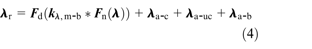
where
The functions
where
2.2.3 Combination of amplitude and wavelength scales
Pairs of wavelength vectors

2.2.4 Parameters for random numbers
For simplicity, the random numbers used for simulating the uncorrelated and correlated contributions introduced above are drawn from normal distributions with mean value
Additive components:
Multiplicative components:
The standard deviation parameter
The uncertainty of the wavelength scale parameters is, for example, 1 nm for the additive components (
The uncertainty of the amplitude scale parameters (
These parameters are not used to generate a realistic measurement uncertainty. Rather, they are used to generate easy-to-use sensitivities that can be used in a linear manner for small measurement uncertainties.
Example: If we use 1 nm for the value of the model parameter for the additive fully correlated wavelength uncertainty component
2.3 Basis function technique
The basis function technique is explained in detail in Kärhäet al.
6
for Fourier basis functions and in Vaskuri et al.
8
for Chebyshev basis functions. The implementation can be found in the MC Toolbox of the open-source Python package 19nrm02
10
in the file
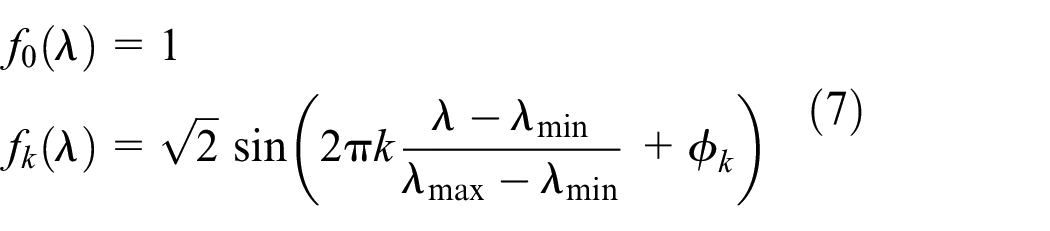
Fourier basis functions
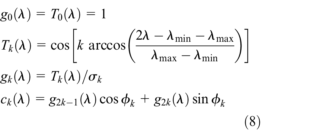
Chebyshev basis functions
where
Based on the generated basis functions
Depending on the Fourier or Chebyshev functions used, different types of basis functions are calculated. A deviation function
The direct influence of a specific basis function order

A comparison with correlations in real datasets in Maham et al.
9
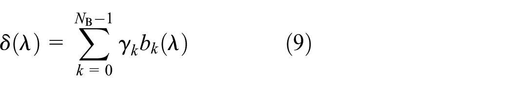
suggests that the summation of the results of the
where
In every trial of the MCS, the random numbers
In the last step, the wavelength (Equation (12)) or amplitude (Equation (13)) data can be modified accordingly by the basis functions:
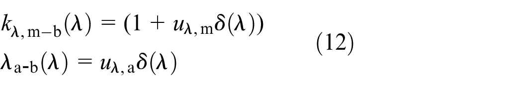
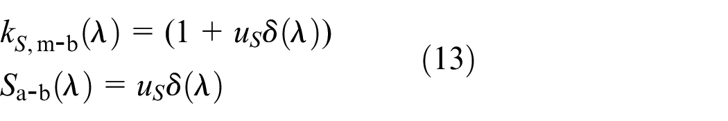
where
The corresponding vectors (
2.4 Connection to physical models
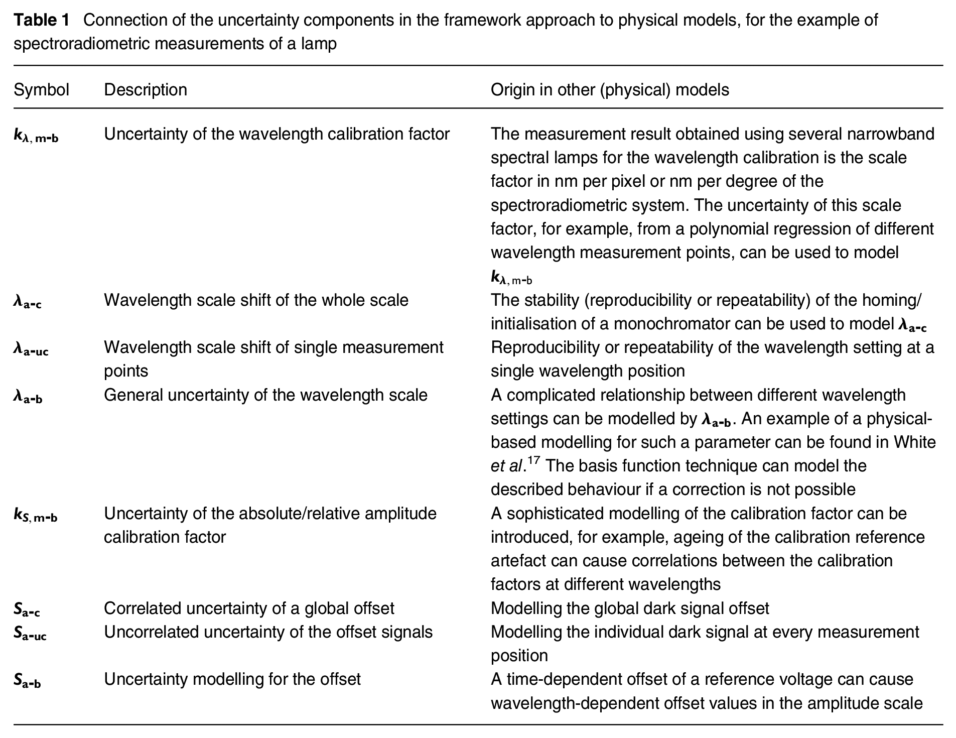
The framework approach can be linked to the physical properties of measurement systems. An overview is given in Table 1 together with the uncertainty components in the framework approach.
Connection of the uncertainty components in the framework approach to physical models, for the example of spectroradiometric measurements of a lamp
3. Comparison of real and modelled results
In Section 3.1, real measurement data, provided by the PTB, are used for the MCS2 path to compare the results with modelled data from the framework approach from the MCS1 path of the simulation as presented in Section 3.2. The reduction of the datasets from the simulation into a form that can be transferred to other users or to other simulation paths is described in Section 3.3. As an example, we calculate tristimulus values and chromaticity data as explained in Section 3.4.
3.1 Real measurement data
During the development of the framework method, the PTB provided a dataset from a real measurement of the spectral irradiance of an FEL lamp. The data consisted of a mean spectral distribution vector
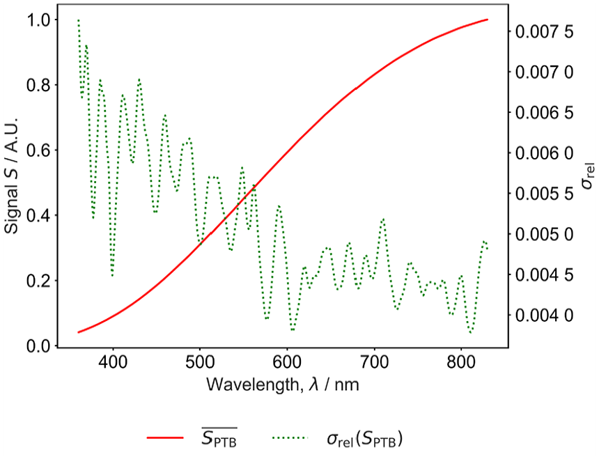
Spectral distribution
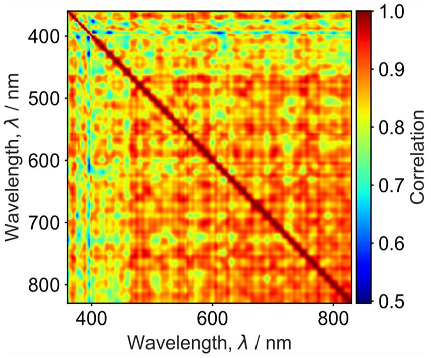
Correlation matrix
The data from PTB were then used to generate a value matrix

3.2 Modelled data using the framework approach
In this study, we used the model as described in this section to perform a sensitivity analysis on the calculated relative luminance, chromaticity coordinates and correlated colour temperature (CCT). Separate MCSs were performed for each source of uncertainty with respect to Equations (3) and (4), with the random number parameters described in Section 2.2, so that the sensitivity of the output values to each source of uncertainty in turn could be calculated. This follows the type of sensitivity analysis proposed by Razavi and Gupta. 7
The spectral distribution of a blackbody at a temperature of 3077 K was used as input quantity for the simulated measurement, to make the simulation as simple as possible. The chosen blackbody temperature is the same as the CCT of the FEL lamp measured at PTB (see Section 3.1) and gives a spectral distribution very close to the relative spectral distribution of the measured lamp. Based on this theoretical blackbody, the amplitude and wavelength values were modified during the MCS as described above (MCS1). With the modified spectral distributions, one can calculate integrated output quantities and study their behaviour during the simulation. Using these simulation data one can estimate the PDFs and statistical parameters for all output quantities, including mean and standard deviation.
Since this assessment is not based on an actual measurement system, we only generate sensitivity values rather than absolute values. This means one can state at the end, for example: The sensitivity coefficient for the chromaticity coordinate x is 0.0006 for every 1 nm correlated error in the wavelength scale.
Starting from a blackbody at 3077 K at a nominal wavelength scale from 360 nm to 830 nm with 1 nm steps, and using the model equations presented previously, we generate
For the amplitude scale, Equation (3), the following parameters are used in the simulation:
For the wavelength scale, Equation (4), the following parameters are used in the simulation:
3.3 Data transfer and interpolation
For data visualisation or the transfer of measurement results to other users, the matrix

Using a non-nominal wavelength scale usually requires interpolation for further calculations. This interpolation of the amplitude vector to regular, equidistant wavelength intervals means that the measurement uncertainties of the wavelength vector are converted to the amplitude values and influence the measurement uncertainties and correlations for the amplitude vector. Care is needed when doing the interpolation, particularly if the amplitude vector is noisy, since artificial spectral structure can be introduced if an inappropriate interpolation method is used. Guidance on interpolation is given in CIE 15:2018, Clause 7.2.3. 14 (Rule of thumb: Interpolate the smooth function and not the noisy one.)
New data pairs

3.4 Calculation and evaluation of integral data
As an example, to show the effect of the different measurement uncertainties (with regard to the parameters of the models introduced above), several integrated quantities (tristimulus values, chromaticity coordinates and CCT) are calculated from the simulated spectral distributions.
According to CIE 15:2018, Clause 7 14 the tristimulus values, X, Y, Z, are calculated with Equation (17) using the nominal wavelength scale.
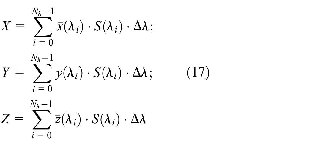
where
Using the spectral distributions generated with the framework approach, the tristimulus values,
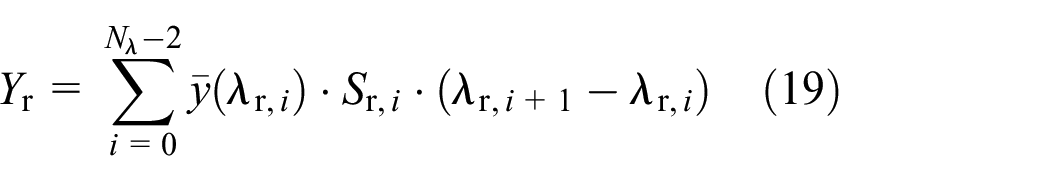
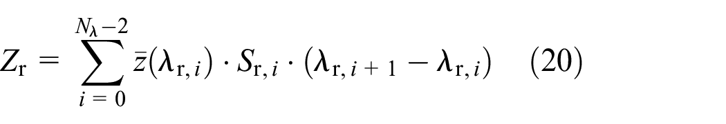
Note that, due to the variation of the wavelength scale in each MC trial depending on the modelling, the wavelength steps are calculated separately for each trial and therefore the integrated values obtained using Equations (18) to (20) are also calculated separately for each trial:

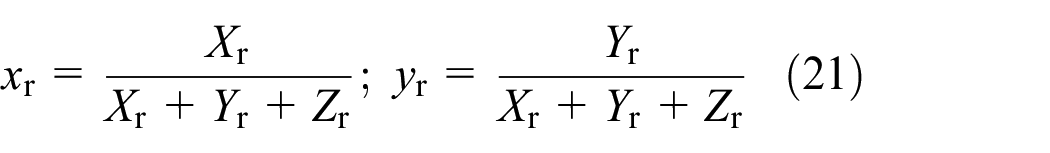
The CCT is calculated from the chromaticity coordinates
4. Results
All diagrams, tables and calculations in the following are based on the open-source Python package 19nrm02
10
and implemented in the Jupyter Notebook
Table 2 shows the result of the MCS1 for the described model settings and the output data relative luminance (Y), chromaticity coordinates (x, y) and CCT (
Evaluation table for the MU calculation using the framework approach in the MCS1
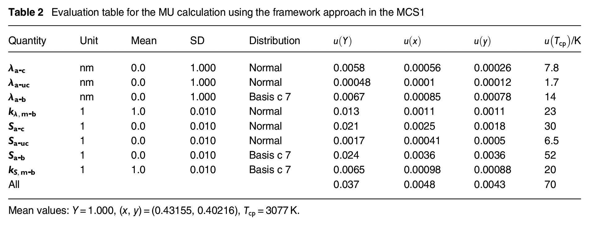
Mean values: Y = 1.000, (x, y) = (0.43155, 0.40216),
Relative luminance: The additive correlated components and the additive partially correlated components (basis functions for both the wavelength and the amplitude scales) have a greater contribution to the uncertainty than the other effects.
Chromaticity coordinates: Uncorrelated contributions of the model average out and correlated additive amplitude component as well as the multiplicative basis function contribution for the wavelength scale and the additive basis function contribution for the amplitude scale are significant.
CCT: Besides all the partially correlated parameters modelled by the basis functions, the correlated additive amplitude component contributes significantly to the uncertainty.
The results of the uncertainty evaluation for the chromaticity coordinates are shown graphically in Figures 4 and 5, in terms of expanded uncertainty ellipsoids. Figure 4 shows the effect of the wavelength scale parameters, and Figure 5 shows the effect of the amplitude scale parameters. The label ‘All’ is used for the results in the last row of Table 2 containing all modelled uncertainty contributions. In addition to the data in Table 2, these plots allow the chromaticity uncertainty and the correlation to be analysed together.
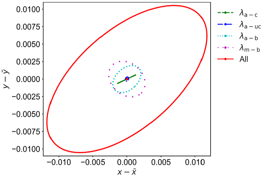
Covariance plots for the chromaticity coordinates based on the wavelength uncertainty contributions
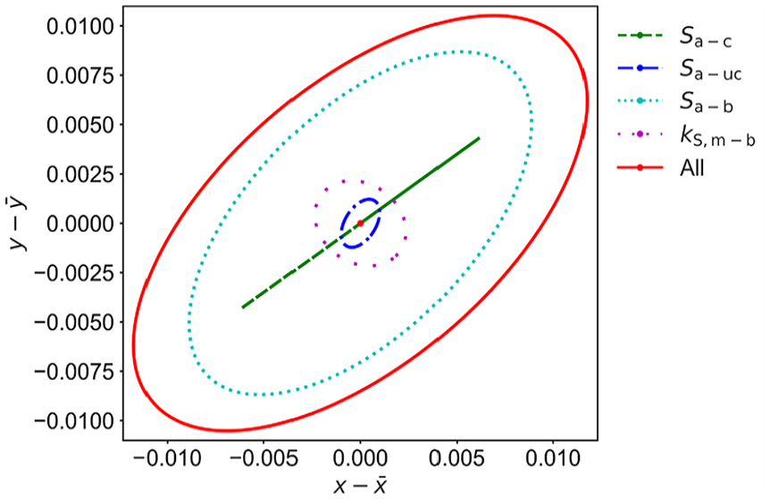
Covariance plots for the chromaticity coordinates based on the amplitude uncertainty contributions
The correlated additive components result in fully correlated chromaticity uncertainties, displayed as a line. The other contributions result in ellipsoids with different principal axis orientations and lengths. A major contribution is the partially correlated amplitude component, which is modelled as an additive basis function.
Figures 6 to 9 show selected correlation matrices of the generated spectral distributions inside the MCS1 based only on the influence of the model parameter
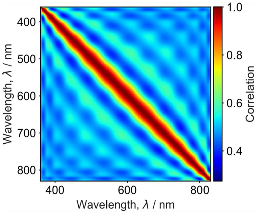
Correlation matrix for the spectral distribution with
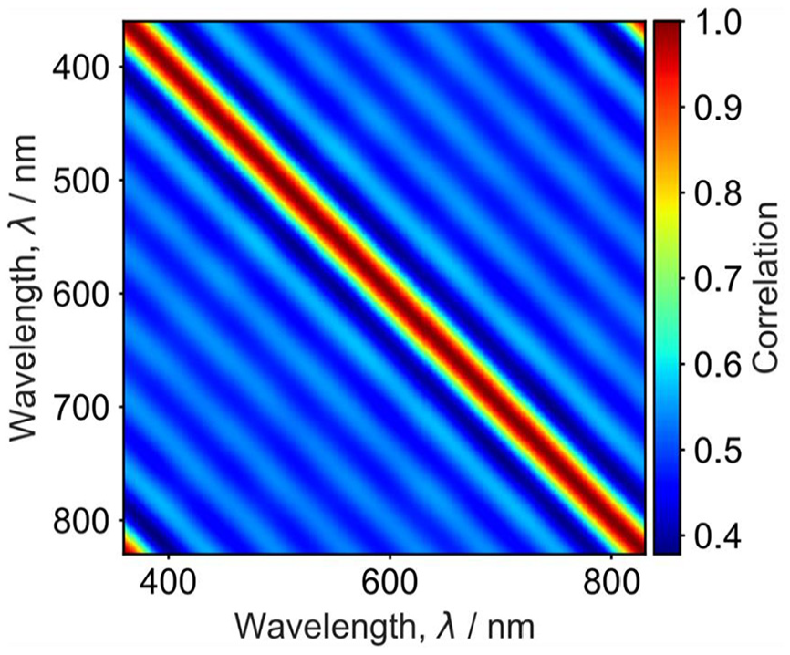
Correlation matrix for the spectral distribution with
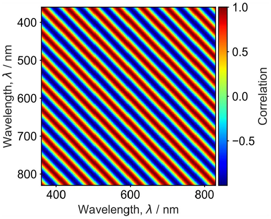
Correlation matrix for the spectral distribution with seventh base function only (Fourier basis functions,
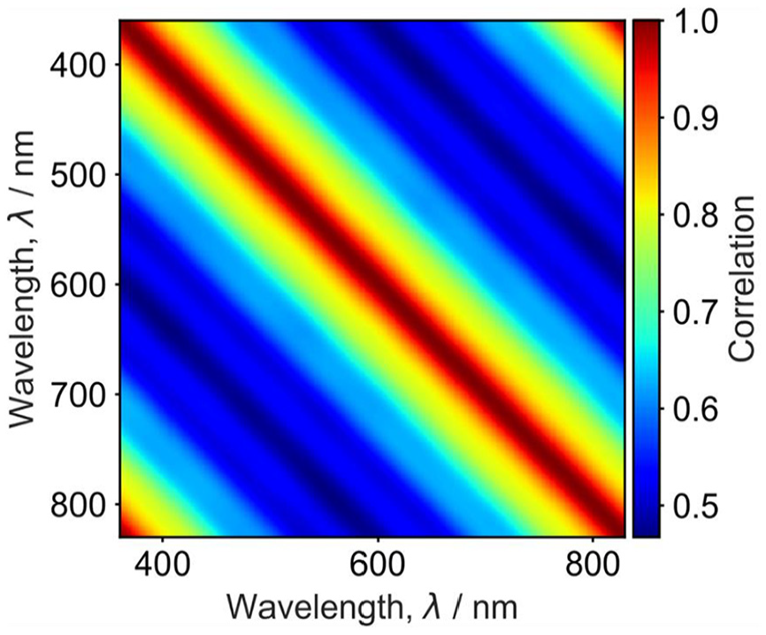
Correlation matrix for the spectral distribution with
The nominal wavelength scale is used for the ordinate and abscissa axes in these plots. For the following examples, one can see that there is only a partial correlation generated by the basis function approach between different wavelength settings and not a full correlation as could be expected.
Figure 6 shows the correlation matrix for the spectral distribution based on the
Figures 6 to 9 indicate different correlation matrices that are also structured completely differently from the measurement results of the PTB, which are shown in Figure 3. The authors cannot yet provide general interpretations of the selected correlation matrices displayed here.
4.1 Evaluation of different basis function numbers and types
Iterating the MCS over several basis function numbers (
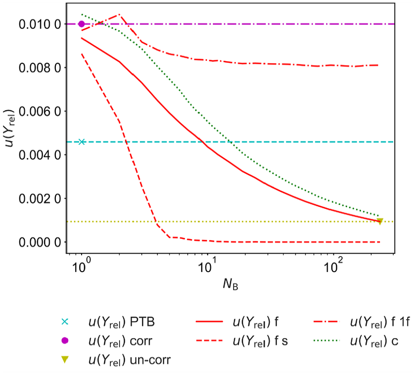
Measurement uncertainty of relative tristimulus value, u(Yrel), as a function of the number of basis functions, NB.
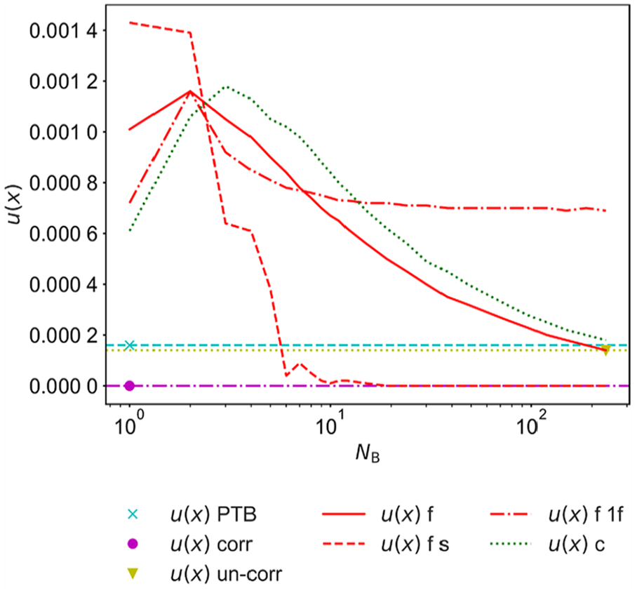
Measurement uncertainty of the chromaticity value, u(x), as a function of the number of basis functions, NB
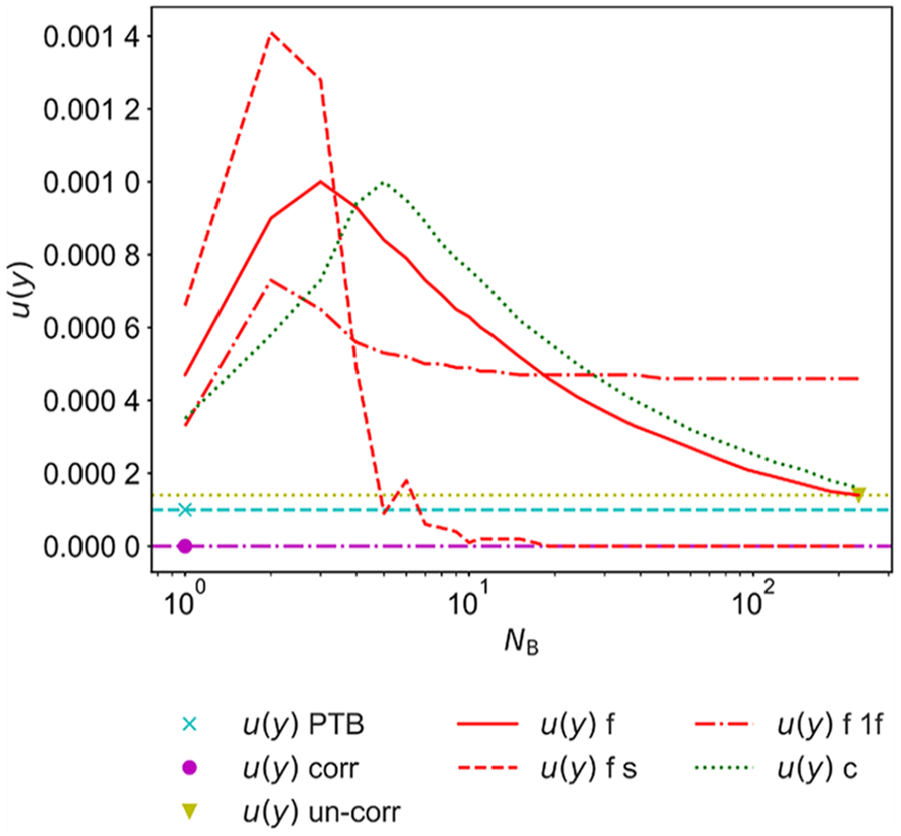
Measurement uncertainty of chromaticity value, u(y), as a function of the number of basis functions, NB
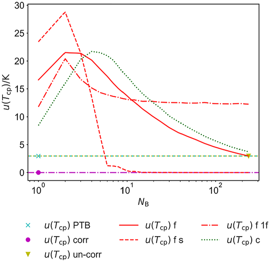
Measurement uncertainty of the correlated colour temperature value, u(Tcp), as a function of the number of basis functions, NB
Figures 10 to 13 show the number of basis functions on the horizontal axis (log scale) and on the vertical axis the measurement uncertainty of different quantities (tristimulus value (Y), chromaticity coordinates
Besides identifying the basis function number that has the maximum impact on the final uncertainty in each case, three specific points are usually of particular interest and marked separately in Figures 10 to 13:
The uncertainties evaluated from the measurement results from PTB are shown as an additional point and a corresponding horizontal line marked with the label ‘PTB’.
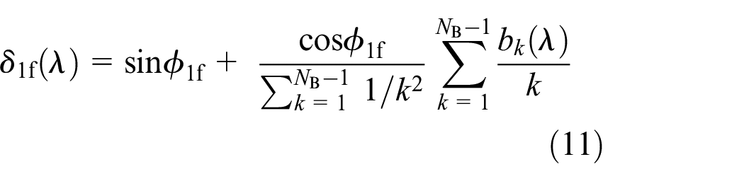
The different basis function techniques are displayed with different graphs and labelled with ‘f’ for the cumulative Fourier basis functions (see Equation (9)), ‘f s’ for a single Fourier basis function (see Equation (10)) and ‘c’ for cumulative Chebyshev basis functions. The one over f approach using Fourier basis functions is labelled with ‘f 1f’ (see Equation (11)).
5. Discussion
The simulations show that, as expected, uncorrelated and fully correlated contributions generally have no significant influence on chromaticity coordinates and the other evaluated quantities. The exception is the contribution from the additive, fully correlated errors in the values of the wavelengths (e.g. caused by the homing/initialising procedure of a monochromator or by the wavelength adjustment of an array spectroradiometer with a few spectral lines only), which makes significant contributions to nearly all investigated output quantities.
However, it was shown by modelling with orthogonal basis functions that partial correlations contribute significantly to the measurement uncertainty. The tristimulus functions change slowly with wavelength and therefore only the long-wave basis functions (i.e. those where
Using single basis functions provides information about the most sensitive frequency for the basis function technique. It is usually observed that ignoring correlations for intermediate spectral frequencies leads to a greater underestimation of the uncertainty. It therefore makes sense to carry out this single basis function analysis and to analyse the results carefully.
6. Conclusion
The framework approach presented in this paper makes it possible to understand the main contributions of the spectral measurement uncertainties to the estimated combined measurement uncertainty and to consider their impact for specific cases. Additionally, this approach identifies possible correlations among the output quantities.
An MCS1 has shown that when evaluating quantities and uncertainties derived using spectral integrations, the fully correlated and uncorrelated errors contribute much less to the uncertainty than the partially correlated errors modelled by the basis functions. As expected, the basis functions with fewer terms (functions with low spectral frequencies representing errors with short autocorrelation length) provide a larger uncertainty in the evaluation of these spectrally integrated quantities and thus provide a reasonable estimate of the maximum uncertainty.
Footnotes
Acknowledgements
A version of this work was also published in the Proceedings of the CIE 2023 Session. We thank Kevin G. Smet for implementing all the photometric and colorimetric functions in the LuxPy Python package, which we used to implement the calculations presented here. We thank Thorsten Gerloff from PTB Germany for providing the measurement data of the FEL lamp, including the beneficial covariance information. Finally, we would like to thank Peter Zwick, Teresa Goodman and the reviewers for their numerous valuable comments during the final correction of the paper.
Declaration of conflicting interests
The authors declared no potential conflicts of interest with respect to the research, authorship, and/or publication of this article.
Funding
The authors disclosed receipt of the following financial support for the research, authorship, and/or publication of this article: This project 19NRM02 RevStdLED has received funding from the EMPIR programme, co-financed by the Participating States and from the European Union’s Horizon 2020 research and innovation programme. Erkki Ikonen wishes to acknowledge support by the Research Council of Finland Flagship Programme, Photonics Research and Innovation (PREIN), decision number: 346529.
Supplemental material
Supplemental material for this article is available online.
References
Supplementary Material
Please find the following supplemental material available below.
For Open Access articles published under a Creative Commons License, all supplemental material carries the same license as the article it is associated with.
For non-Open Access articles published, all supplemental material carries a non-exclusive license, and permission requests for re-use of supplemental material or any part of supplemental material shall be sent directly to the copyright owner as specified in the copyright notice associated with the article.