Sage Journals: Discover world-class research

Abstract

Flicker and stroboscopic effects caused by a temporally modulated light source may be harmful for the human visual system. Standardized measurement methods have been developed for the related temporal light artefacts of LED luminaires. It was found out that the performance of the International Electrotechnical Commission (IEC) recommended flickermeter implementation is highly dependent on sampling frequency. Novel digital implementations for the flickermeter and stroboscopic effect visibility measure (SVM) were created to remove any inaccuracies. The performance of the novel Aalto implementations does not depend on the sampling frequency when running the test waveforms of the IEC standard through the implementations. As compared with the IEC recommended digital implementations, Aalto flickermeter decreases the average error related to the test waveforms from −0.05 to +0.003, and Aalto SVM meter also decreases the average error by almost two orders of magnitude.

1. Introduction

Different operating principles of light sources based on LEDs and incandescent lamps cause their temporal light modulation (TLM) behaviour to be significantly different. The TLM properties produce temporal light artefacts (TLA) that are visible effects in the human visual system. TLAs have been linked to some adverse effects to humans.^1,2 The EU Ecodesign Regulation sets limits to two of the TLA metrics: the short-term flicker severity index $P_{st}^{LM}$ and the stroboscopic effect visibility measure M_VS (SVM). LED manufacturers need to follow the regulation when producing luminaires for the EU area.³

The values of $P_{st}^{LM}$ and M_VS can be determined by feeding a measured light waveform from a luminaire to a digital TLA meter.⁴ There are freely available MATLAB implementations recommended by International Electrotechical Commission (IEC) TR 61547 for flickermeter⁵ and IEC TR 63158 for SVM meter.^5,6 These can be found as MATLAB toolboxes for $P_{st}^{LM}$ and M_VS respectively.^7,8

In this work, we describe anomalies found in the IEC recommended flickermeter implementation caused by built-in MATLAB functions butter() and filter(). These functions do not follow the analogue response in the frequency band of interest in the IEC recommended implementation. This effect was noticed at the sampling frequency of 50 kHz and further studied using sampling frequencies between 40 kHz and 100 kHz. Because of this reason, we implemented novel flicker and SVM meters to remove any anomalies in the TLA characterization results. These Aalto implementations decrease the average deviations from the expected values by an order of magnitude in the case of flickermeter and by almost two orders of magnitude in the case of SVM meter.

2. Flickermeter and stroboscopic effect visibility meter

We first describe the principles of digital implementations of the short-term flicker severity index and stroboscopic effect visibility measure. Both meters are defined in related standards^5,6 and consist of four blocks A to D that handle different physiological effects in the human vision system. Block diagrams are presented in Figures 1 and 3 for the flickermeter and stroboscopic effect visibility meter, respectively.

Figure 1

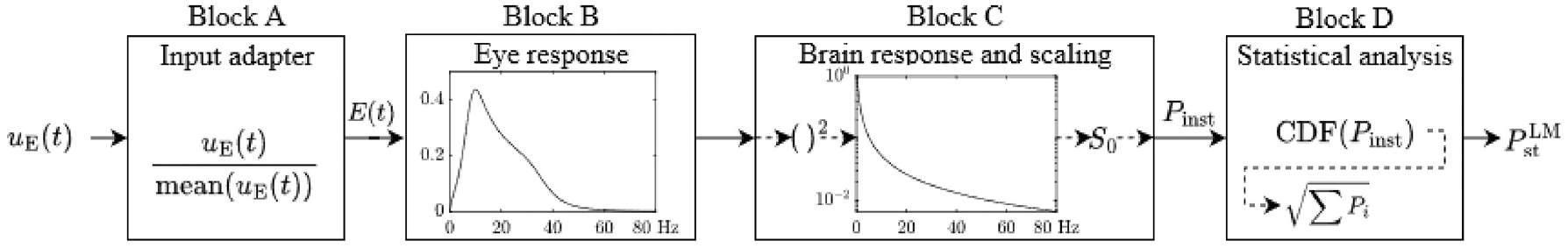
Drawing of a block diagram of the flickermeter as it is described⁵ in IEC TR 61547

2.1 Light flickermeter

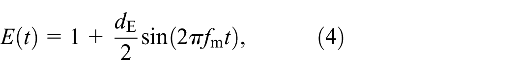
Block A in the flickermeter, as can be seen in Figure 1, works as an input adapter. The output of Block A is the normalized light waveform E(t).^5,9

In Block B, the human eye response is simulated by using three different filters. Firstly, the signal goes through a first-order high-pass filter. The transfer function of the high-pass filter in Laplace domain is defined as shown in equation (1):

F_{HP} (s) = \frac{τ_{HP} s}{τ_{HP} s + 1}

(1)

where s = j $ω$ is the Laplace variable, with j as the imaginary unit, and $ω = 2 π f_{m}$ accounts for the frequency component $f_{m}$ of the signal. In Equation (1), $τ_{HP} = 3.18 s$ is the filter time constant.^5,9 Next, the light waveform is fed through a sixth-order low-pass Butterworth filter F_LPBW(s). This filter has a cut-off frequency of 35 Hz with mains frequency of 50 Hz. Butterworth filter has been chosen, as it has the flattest response at the desired passband. The sixth-order filter was selected to achieve −50 dB attenuation at double of the mains frequency.¹⁰

The third and final filter in Block B is a specialized bandpass filter $F_{WF}^{LM} (s)$ with a peak at 10 Hz. The filter is defined^1,7 using equation (2):

F_{W F}^{L M} (s) = \frac{0.041661 s^{4} + 44.758 s^{3} + 2715.6 s^{2} + 29 839 s}{s^{4} + 196.32 s^{3} + 1781 s^{2} + 534 820 s + 3 505 380} ..

(2)

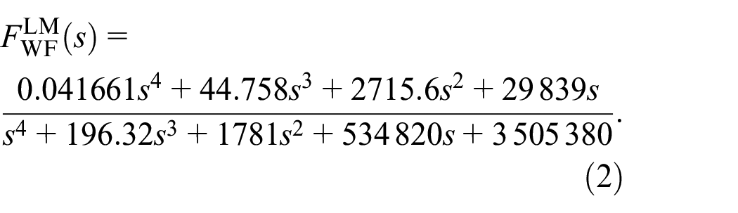
Equation (2) has the form given in IEC TR 61547-1, and it represents the frequency response of an average human eye to the flicker signal.⁵ After these three filters, the input waveform is highly attenuated outside the most effective range of 5 Hz to 30 Hz, which can be seen in the black curve in Figure 2. The digital implementation of these filters is described in more detail in Appendix A.

Figure 2

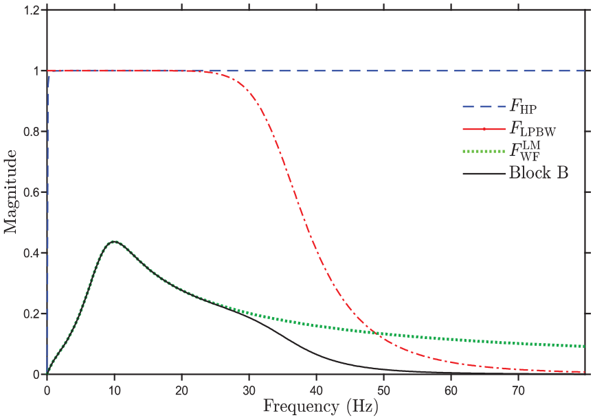
Linear scale amplitudes for the filters in Block B, and the total amplitude of all filters

Block C of the light flickermeter is responsible for modelling the eye–brain response to the output signal from Block B. Block C is identical to Block 4 in the IEC 61000-4-15 flickermeter.⁵ Firstly, the signal is squared to implement the nonlinearity of perception of flicker happening in the transfer phase from eye to brain.^9,10 After this, the brain memory storage effect is modelled with a first-order low-pass filter defined as:

F_{LP} (s) = \frac{1}{τ_{LP} s + 1},

(3)

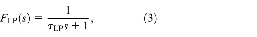
where $τ_{LP} = 300 ms$ is the time constant. This filter acts as a sliding mean filter that merges the fast changes in the flicker severity.¹⁰ The resulting waveform is the unscaled instantaneous flicker sensation.⁵ Digital implementation of the filter of Equation (3) is described in Appendix A.

Maximum instantaneous flicker should get a value of $P_{inst} = 1$ with illuminance waveform:

E (t) = 1 + \frac{d_{E}}{2} \sin (2 π f_{m} t),

(4)

where $d_{E} = 0.006832$ is the peak-to-peak amplitude of the sinusoidal modulation at frequency $f_{m} = 8.8 Hz$ .⁵ This is achieved by multiplying the filtered signal with a scaling factor S₀, dependent on filters described above. The output of Block C is the instantaneous flicker sensation $P_{inst}$ .⁵ Equation (4) is later used in creation of the test waveforms.

Finally, in Block D, the $P_{st}^{LM}$ value is calculated from the $P_{inst}$ by conducting statistical analysis. This is done by dividing $P_{inst}$ into 2¹² vertical bins and then applying the cumulative distribution function. The $P_{st}^{LM}$ is now calculated as:

P_{s t}^{L M} = \sqrt{0.0314 P_{0.1} + 0.0525 P_{1 S} + 0.0657 P_{3 S} + 0.28 P_{10 S} + 0.08 P_{50 S}}

(5)

where $P_{q}$ are the values of $P_{inst}$ above which $q %$ of the $P_{inst}$ values locate.¹¹ Sudden changes in the cumulative probability are considered by smoothing the values. These are notated by suffix S and are smoothed as defined by Equations (6) to (9)¹¹:

P_{1 S} = \frac{P_{0.7} + P_{1} + P_{1.5}}{3}

(6)

P_{3 S} = \frac{P_{2.2} + P_{3} + P_{4}}{3}

(7)

P_{10 S} = \frac{P_{6} + P_{8} + P_{10} + P_{13} + P_{17}}{5}

(8)

P_{50 S} = \frac{P_{30} + P_{50} + P_{80}}{3}

(9)

2.2 Stroboscopic effect visibility meter

Function of Block A in the SVM meter as can be seen in Figure 3 is the same as in the flickermeter. Block B of the SVM meter takes the temporal light waveform and converts it to frequency spectrum. This is achieved by Hanning windowing and taking the discrete Fourier transform (DFT). Windowing was utilized to remove the effects of spectral leakage in the following Fourier analysis of the spectrum. The spectral leakage in this case would be caused by possible non-integer number of periods of light waveform in the sampled data. As DFT considers the sampled data as a discrete periodic signal, it will join the first and last datapoints together. This will cause a phase-shift in the endpoint boundaries of the signal in the case of sampled data consisting of non-integer number of periods.^12,13

Figure 3

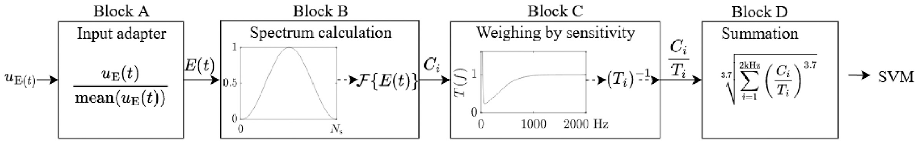
Drawing of a block diagram of the SVM meter as it is described⁶ in IEC TR 63158

Hanning windowing was selected in this case as it is recommended by both Commission International de l’Éclairage (CIE) and IEC.^2,6 The Hanning window is given as:

w_{Hanning} = \sin^{2} (\frac{π n}{N_{s}}), 0 \leq n \leq N_{s}

(10)

where $n$ is the sample index and $N_{s}$ is the number of samples.¹² In the Aalto SVM meter, windowing was achieved by using Equation (10). Hanning window achieves the windowing task by reducing the amplitude at both ends of the signal, smoothing the transition from the end of the signal back to the beginning. This windowing in time domain causes the signal to be attenuated and needs a gain correction factor of 2, which was implemented in the code.^12,13

Because Hanning window is used to attenuate both ends of the signal, zero-padding is only utilized to ensure that the measured signal contains an integer number of periods. The Aalto SVM meter utilizes MATLAB built-in peak-finding algorithm, with a minimum peak distance of 1 Hz, as CIE recommends.² Block B produces the normalized frequency spectrum $C_{i}$ at frequency f_i as the output.

Block C weights the frequency spectrum from Block B with the visibility threshold function for SVM. This is defined as:

T_{i} = \frac{1}{1 + e^{- a (f_{i} - b)}} + 20 e^{- \frac{f_{i}}{c}}

(11)

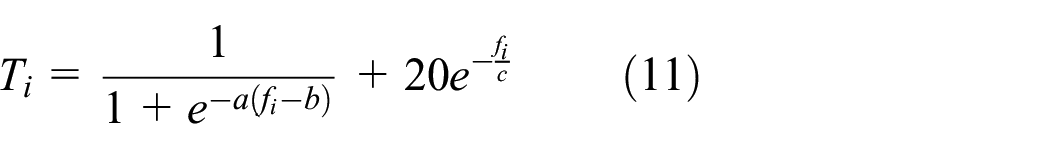
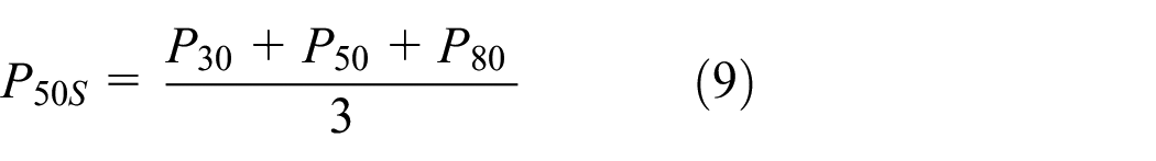
where a = 0.00518s, b = 306.6 Hz, and c = 10 Hz.⁶ The threshold function of Equation (11) is defined in the range 0 Hz to 2000 Hz. The frequency spectrum $C_{i}$ is divided by $T_{i}$ , which produces the output of Block C. Block D consists of only the summation of the weighted spectrum. SVM value is calculated as:

M_{VS} = \sqrt[3.7]{\sum_{i = 1}^{N} {(\frac{C_{i}}{T_{i}})}^{3.7}}

(12)

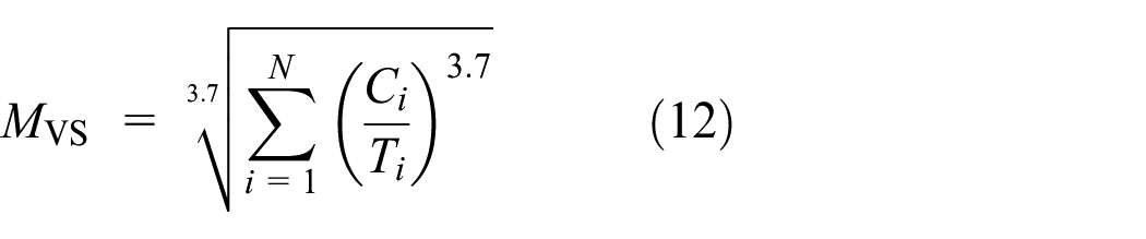
where the summation of Equation (12) covers frequency components up to 2 kHz.⁶ The Aalto SVM meter is designed to be used with long-duration light waveform (>20 s) with high sampling frequency (up to 100 kHz).

3. Anomalies in the IEC recommended implementation of light flickermeter

In the IEC recommended implementation of flickermeter, we found out that there are problems with the implementation of filters in blocks B and C.⁷ These were found to be related to the MATLAB functions butter() and filter(), used to create the filtering. Figure 4 compares the analogue response and two digitized responses produced by the Butterworth filters of MATLAB butter() function and by using Tustin’s method to create Butterworth filters.¹² The filter transfer function given by Tustin’s method can be found as Equation (A3) of Appendix A. We see that the signal given by butter() function does not follow the analogue response curve of the Butterworth filter. This is likely due to the way butter() is implemented in the IEC recommended implementation which does not follow the instruction by MATLAB manual.¹⁴

Figure 4

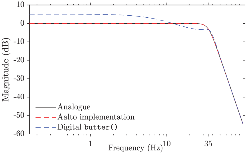
Response curves for sixth-order low-pass Butterworth filter implementations. Black curve under the dashed red line is the theoretical analogue response

To fix these problems, we created a novel MATLAB implementation for the light flickermeter.¹⁵ In the Aalto implementation, the filter transfer functions that were earlier created using butter() function were replaced with filter transfer functions using zero-pole-gain (ZPK) representation in Z-domain as described in Appendix A. The digital ZPK filter representation used with Tustin’s method accurately follows the analogue response curve of the sixth-order Butterworth filter as can be seen in Figure 4.

We did not find any anomalies on the same scale in the IEC recommended SVM meter as in the IEC recommended light flickermeter, but nevertheless decided to recreate the MATLAB code for M_VS following the IEC standard⁶ to see if we could produce better results for the SVM meter as well. The Aalto SVM meter¹⁵ was implemented without using any modules of earlier implementations but following the related IEC standard.⁶

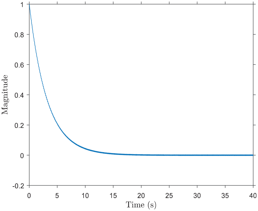
4. Avoiding transient effects

In the IEC standard,⁵ it is recommended to remove the first 60 s from the $P_{inst}$ data to reduce the effects from the transient period. In IEC TR 61547 Table 1, it is stated that the illuminance adapter in Block A is the dominating factor in the filter’s transient response.⁵ We evaluated the behaviour of the transient period within the modulation frequency ranges of the light flickermeter and stroboscopic visibility meter test waveforms, that is, from 0.3 Hz to 1900 Hz and varying the modulation depth between 0 and 1, using Equation (4). During testing, the actual length of this transient period in the Aalto implementation was found out to be less than 20 s with all the waveforms evaluated. An example result can be seen in Figure 5. Because of this, the Aalto implementation disregards only the first 20 s of the data, instead of the full 60 s as recommended in Reference 5.

Table 1

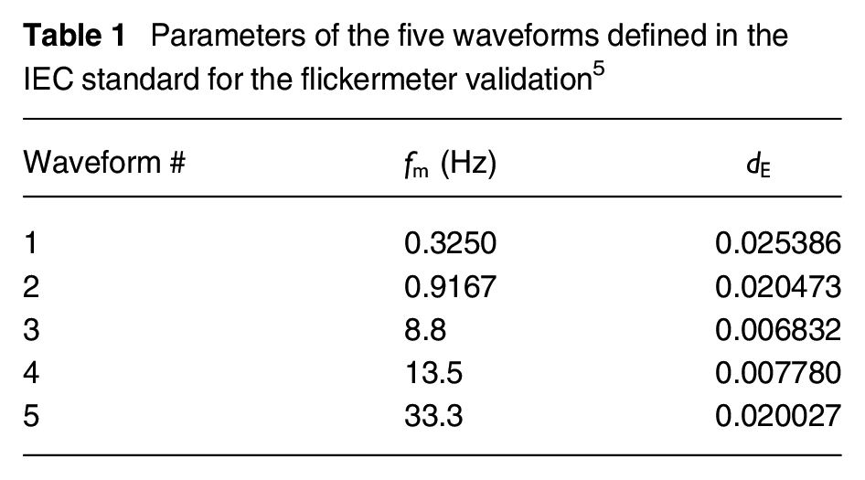
Parameters of the five waveforms defined in the IEC standard for the flickermeter validation⁵

Waveform #	$f_{m}$ (Hz)	$d_{E}$
1	0.3250	0.025386
2	0.9167	0.020473
3	8.8	0.006832
4	13.5	0.007780
5	33.3	0.020027

Figure 5

An example of the transient period of signal going through the input adapter in Block A of Figures 1 and 3 with modulation frequency 8.8 Hz and modulation depth 0.006832

5. Validation of flicker and SVM meter implementations

The validation of the Aalto implementations was conducted with the given test waveforms of the IEC standards^5,6 for the flickermeter and SVM meter.

5.1 Flickermeter validation

In the case of light flickermeter, the IEC standard⁵ gives five different waveforms defined by their modulation frequencies and their relative modulation amplitudes. Defined waveform parameters are shown in Table 1.

IEC TR 61547-1 gives in Section 8.2 seven factors α = 1/4, 1/2, 1, 2, 3, 4 and 5 for scaling the $d_{E}$ values of Table 1 by multiplication, which in the end gives 35 different test cases for flickermeter validation. The values α are the reference values which the digital implementations should produce for each test case.⁵

The results for flickermeter validation are shown in Table 2. IEC deviations are mostly negative and Aalto deviations are positive. This difference is due to the internal biases in the implementations. The bias in the IEC implementation seems to change significantly depending on the modulation frequency of the waveform. As waveform 5 has the highest modulation frequency, it also has the highest flicker value resulting in positive deviations. This Aalto flickermeter implementation outperforms the IEC recommended implementation with all reference waveforms. On the average, the deviation is decreased from −0.05 to +0.003 when moving from the IEC recommended implementation to the Aalto flickermeter implementation.

Table 2

Deviations of the IEC recommended flickermeter and Aalto flickermeter from the target values in absolute units for each five waveforms in Table 1

Target value $α$	Deviation from the target value
	Waveform 1		Waveform 2		Waveform 3		Waveform 4		Waveform 5
	IEC	Aalto	IEC	Aalto	IEC	Aalto	IEC	Aalto	IEC	Aalto
1/4	−0.0100	0.0007	−0.0105	0.0004	−0.0096	0.0002	−0.0019	0.0003	0.0057	0.0009
1/2	−0.0197	0.0012	−0.0206	0.0005	−0.0206	0.0001	−0.0024	0.0004	0.0111	0.0015
1	−0.0401	0.0023	−0.0417	0.0009	−0.0411	0.0001	−0.0044	0.0007	0.0201	0.0029
2	−0.0849	0.0045	−0.0815	0.0018	−0.0803	0.0002	−0.0116	0.0014	0.0433	0.0053
3	−0.1375	0.0068	−0.1287	0.0026	−0.1262	0.0002	−0.0212	0.0021	0.0551	0.0072
4	−0.1802	0.0090	−0.1793	0.0035	−0.1660	0.0003	−0.0207	0.0028	0.0729	0.0087
5	−0.1939	0.0113	−0.2062	0.0043	−0.1892	0.0004	−0.0168	0.0035	0.1074	0.0098

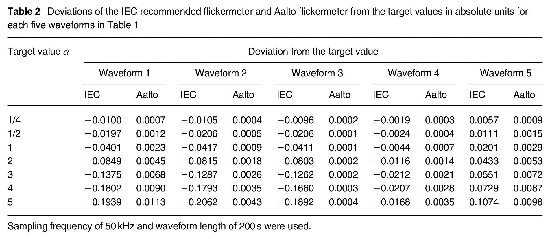
Sampling frequency of 50 kHz and waveform length of 200 s were used.

We also studied the effect of the sampling frequency used for the measurement of light waveform. In Figure 6, the average deviations from the α values are shown as functions of the sampling frequency. Both digital implementations produce similar results for sampling frequencies from 4 kHz to 25 kHz. After 30 kHz, the Aalto implementation starts to outperform the IEC recommended implementation, and at 50 kHz the IEC recommended implementation starts to produce significantly larger deviations than the Aalto implementation. Aalto implementation gives stable results over the 4 kHz to 100 kHz range. At 100 kHz modulation frequency, the average deviation is 0.0028 with the Aalto Implementation.

Figure 6

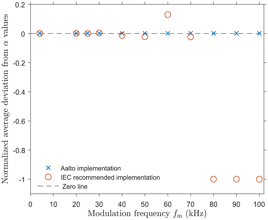
Average deviations from the expected values when using different sampling frequencies. In each case, the deviation is normalized by the value of α

5.2 SVM meter validation

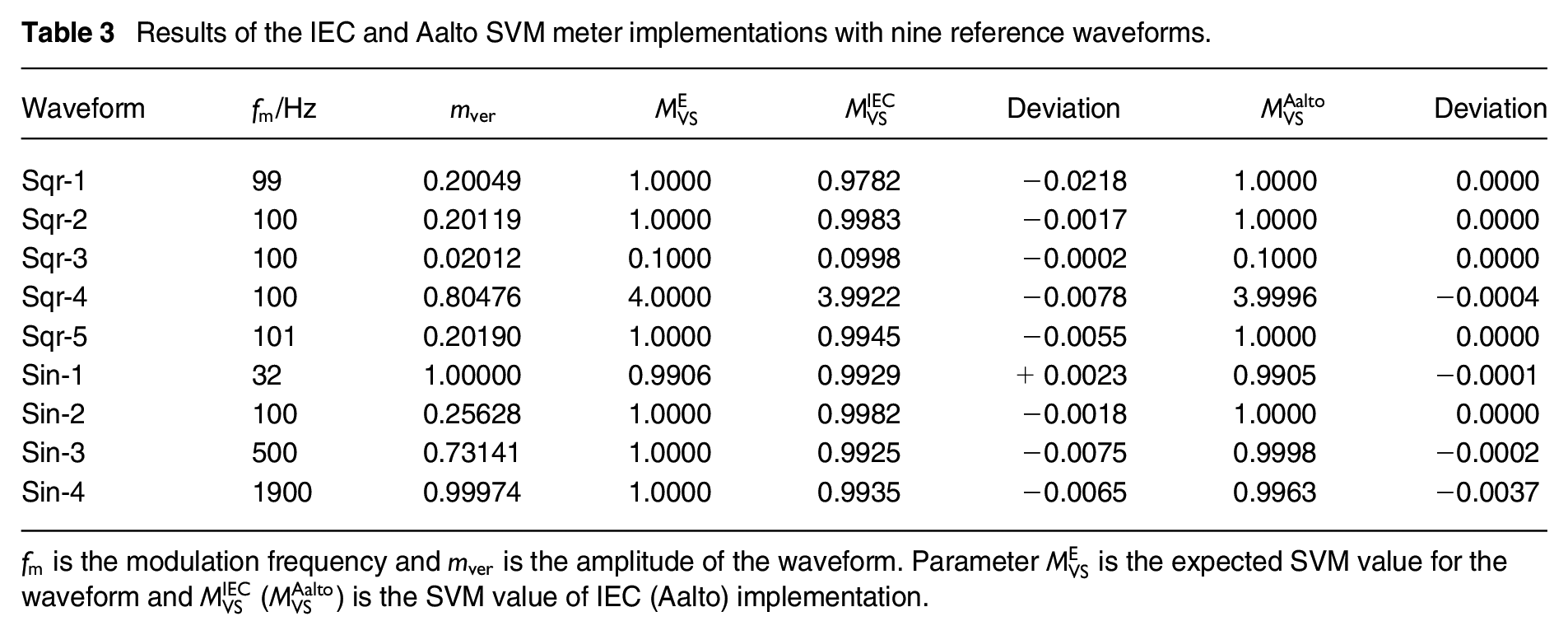
For the SVM meter there are nine different test waveforms.⁶ These waveforms consist of five square waves (Sqr) and four sinusoidal waveforms (Sin) that are defined by their modulation frequencies and amplitudes. The waveforms and results with the IEC recommended implementation and the Aalto implementation can be seen in Table 3. Except for the highest frequency of 1900 Hz, the deviations of Aalto implementation from the expected values $M_{VS}^{E}$ are considerably smaller than those of the IEC recommended implementation. The absolute values of deviations decreased, on the average, from 0.0074 to 0.0001 for square waves, and from 0.0045 to 0.0010 for sine waves when using the Aalto implementation of the SVM meter.

Table 3

Results of the IEC and Aalto SVM meter implementations with nine reference waveforms.

Waveform	$f_{m}$ /Hz	$m_{ver}$	$M_{VS}^{E}$	$M_{VS}^{IEC}$	Deviation	$M_{VS}^{Aalto}$	Deviation
Sqr-1	99	0.20049	1.0000	0.9782	−0.0218	1.0000	0.0000
Sqr-2	100	0.20119	1.0000	0.9983	−0.0017	1.0000	0.0000
Sqr-3	100	0.02012	0.1000	0.0998	−0.0002	0.1000	0.0000
Sqr-4	100	0.80476	4.0000	3.9922	−0.0078	3.9996	−0.0004
Sqr-5	101	0.20190	1.0000	0.9945	−0.0055	1.0000	0.0000
Sin-1	32	1.00000	0.9906	0.9929	+0.0023	0.9905	−0.0001
Sin-2	100	0.25628	1.0000	0.9982	−0.0018	1.0000	0.0000
Sin-3	500	0.73141	1.0000	0.9925	−0.0075	0.9998	−0.0002
Sin-4	1900	0.99974	1.0000	0.9935	−0.0065	0.9963	−0.0037

$f_{m}$ is the modulation frequency and $m_{ver}$ is the amplitude of the waveform. Parameter $M_{VS}^{E}$ is the expected SVM value for the waveform and $M_{VS}^{IEC}$ ( $M_{VS}^{Aalto}$ ) is the SVM value of IEC (Aalto) implementation.

6. Conclusions

The currently available MATLAB implementation of the flickermeter recommended by the IEC standard has problems related to the implementation of filters. They were solved by creating a novel Aalto implementation of the flickermeter in MATLAB using robust mathematical methods. Along with the flickermeter, a novel Aalto SVM meter implementation was created following similarly robust methods.

The performance of the IEC recommended flickermeter implementation is highly dependent on the sampling frequency. Up until 30 kHz, both flickermeter implementations work fine, but with sampling frequencies above 50 kHz, the IEC recommended implementation was found not to work as intended. Aalto flickermeter was shown to produce stable results with sampling frequencies up to 100 kHz when using the test waveforms of the IEC standard.

Aalto flickermeter implementation decreased the errors by an order of magnitude, on average, as compared with the IEC recommended flickermeter, when using the test waveforms. In the SVM meter implementation, Aalto SVM meter decreased the average deviation from the target values by almost two orders of magnitude for the test waveforms when comparing to the IEC recommended SVM meter.

Footnotes

Appendix

Acknowledgements

We would like to thank Carsten Dam-Hansen for pointing out the importance of accurate specification of the amplitude of the SVM test waveforms. This work has been carried out in project 20NRM01 MetTLM that has received funding from the EMPIR program co-financed by the participating states and the European Union’s Horizon 2020 research and innovation program. We also acknowledge support by the Academy of Finland Flagship Programme, Photonics Research and Innovation (PREIN), decision number: 320167.

Declaration of conflicting interests

The authors declared no potential conflicts of interest with respect to the research, authorship, and/or publication of this article.

Funding

The authors disclosed receipt of the following financial support for the research, authorship, and/or publication of this article: This work has been carried out in project 20NRM01 MetTLM that has received funding from the EMPIR program co-financed by the participating states and the European Union’s Horizon 2020 research and innovation program. We also acknowledge support by the Academy of Finland Flagship Programme, Photonics Research and Innovation (PREIN), decision number: 320167.

ORCID iDs

V Mantela

J Askola

References

Institute of Electrical and Electronics Engineers. IEEE Recommended Practices for Modulating Current in High-Brightness LEDs for Mitigating Health Risks to Viewers. New York, NY, USA: IEEE 1789-2015. 2015.

Commission International de l’Éclairage. Visual Aspects of Time Modulated Lighting Systems – Definitions and Measurement Models. CIE TN 006:2016. Vienna: CIE, 2016.

Directorate-General for Energy. Commission Regulation (EU) 2019/2020 of 1 October 2019 Laying Down Ecodesign Requirements for Light Sources and Separate Control Gears Pursuant to Directive 2009/125/EC of the European Parliament and the Council and Repealing Commission Regulations, Brussels, Belgium: European Union. 2019.

Commission International de l’Éclairage. Guidance on the Measurement of Temporal Light Modulation of Light Sources and Lighting Systems. CIE TN 012:2021. Vienna: CIE, 2021.

International Electrotechnical Commission. Equipment for General Lighting Purposes – EMC Immunity Requirements – Part 1: Objective Light Flickermeter and Voltage Fluctuation Immunity Test Method. IEC TR 61547-1:2020 Ed. 3.0. Geneva, Switzerland: IEC, 2020.

International Electrotechnical Commission. Equipment for General Lighting Purposes – Objective Testing Method for Stroboscopic Effects of Lighting Equipment. Geneva, Switzerland: IEC TR 63158:2018 Ed. 1.0. IEC, 2018.

Banerjee

Light flicker assessment toolbox. Retrieved 23 May 2021 from https://www.mathworks.com/matlabcentral/fileexchange/63445-light-flicker-assessment-toolbox

Banerjee

Stroboscopic effect visibility measure toolbox. Retrieved 23rd May 2021 from https://www.mathworks.com/matlabcentral/fileexchange/59242-stroboscopic-effect-visibility-measure-toolbox

International Electrotechnical Commission. Testing and Measurement Techniques – Flickermeter – Functional and Design Specifications. IEC 61000-4-15 Ed. 2.0. Geneva, Switzerland: IEC, 2010.

10.

Mombauer

Calculating a new reference point for the IEC-flickermeter. European Transactions on Electrical Power 1998; 8: 429–436.

11.

Drapela

Slezingr

A light flickermeter – Part I: Design. Proceedings of the 11th International Scientific Conference Electric Power Engineering, Brno, Czech Republic, 2010: 453–458.

12.

Oppenheim

Shafer

RW.

Discrete-Time Signal Processing. 3rd Edition. New Jersey, USA: Prentice Hall, 2010.

13.

Harris

FJ.

On the use of windows for harmonic analysis with the discrete Fourier transform. Proceedings of the IEEE 1978; 66: 51–83.

14.

Mathworks. Butterworth filter design. Section: More about – Limitations. Retrieved 26 May 2023 from https://se.mathworks.com/help/signal/ref/butter.html#d124e9521

15.

Nordlund

Mantela

Aalto implementations for flickermeter and SVM meter [Online database]. Retrieved February 2022 from https://github.com/MantelV/Aalto-implementations-for-flickermeter-and-SVM-meter

16.