Sage Journals: Discover world-class research

Abstract

After dark, pedestrians may experience discomfort from glare caused by outdoor lighting. While several models for measuring discomfort have been proposed, there is no consensus as to which model should be used. The performances of different models were investigated using datasets from four independent studies, comparing the degree of association between model predictions and subjective ratings, and the ability of a model to distinguish between discomfort and non-discomfort situations. The models tested are those proposed by Petherbridge and Hopkinson in 1950, Schmidt-Clausen and Bindels in 1974, Bullough et al. in 2008 and Lin et al. in 2014 and 2015. They also include two quantities: direct illuminance at the eye from the glare source and average source luminance. Of the models tested, the best performance was found using either the model proposed by Bullough et al. in 2008 or by direct illuminance at the eye.

1. Introduction

Glare arises when part of the visual field, a light source or a surface, is much brighter than the rest of the field. Two common visual impacts of glare are disability and discomfort, and these outcomes may persist individually or together. Disability from glare is a situation where the glare source impairs visibility or visual performance.^1,2 Discomfort from glare is a situation when the observer feels visual discomfort due to the glare source but does not necessarily experience a visual disability.^1,2 The induced discomfort can be described as a sensation of annoyance or pain from a glare source located within the field of view. The magnitude of discomfort is usually described on a scale ranging from barely noticeable to unbearable.

One aim of a lighting design is to minimize discomfort for pedestrians (and other road users) and to do so designers might refer to the quantitative recommendations of lighting guidance documents. For interior lighting, glare limits such as the Unified Glare Rating (UGR) are calculated based on the luminances of light sources and their background, the size subtended by each light source at the observer’s eye and its position in the visual field: a UGR of 22 is the threshold for unacceptable glare in office and classroom spaces, and hence, the design targets a UGR of less than 22.^3,4

Several models for predicting discomfort from road lighting have been proposed. CIE 243:2021 reviews various models,⁵ but some models may not apply to pedestrians because they include terms related to drivers. Examples include the number of luminaires per kilometre in the Glare Control Mark model,⁶ the considered road area in Vos’s Glare Index,⁷ and duration of light pulse in Lehnert’s model.⁸ Other models described in CIE 243:2021 might be relevant to pedestrian applications but are not discussed in this article because either we did not have access to their underlying studies or the underlying study was not published in English. The remaining models that did not include terms specific to drivers might be applicable to pedestrians, given that the eye does not discriminate between purposes of lighting.^9–13

While multiple models can be relevant for pedestrian applications, it remains unclear which model performs better and can be used in practice. The objective of this article is to evaluate candidate models including luminance-contrast-based models by Petherbridge and Hopkinson and Lin et al.,^9,10 a model by Schmidt-Clausen and Bindels that uses both luminance and illuminance quantities,¹¹ illuminance-based models by Bullough et al. and Lin et al.,^12,13 as well as two single-term models: direct illuminance from the source and average luminance. These models vary in complexity due to differences in the number of variables considered and the type of quantities used (luminance and/or illuminance).

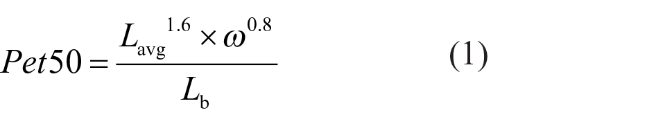
The first model is that proposed by Petherbridge and Hopkinson.⁹ In a laboratory experiment, they varied average source luminance (L_avg), source size in solid angle (ω), source eccentricity (θ) and source shape, and evaluated discomfort by asking subjects to adjust background luminance (L_b) to meet four discomfort criteria: just intolerable, just uncomfortable, just acceptable and just imperceptible. Eccentricity in this context refers to the angular displacement of the source from the point of fixation. Their model (see Equation (1)), referred to as Pet50, is based on the contrast between the luminances of the source and its background, with account also taken of the size subtended by the source at the observer’s eyes.

P e t 50 = \frac{{L_{avg}}^{1.6} \times ω^{0.8}}{L_{b}}

(1)

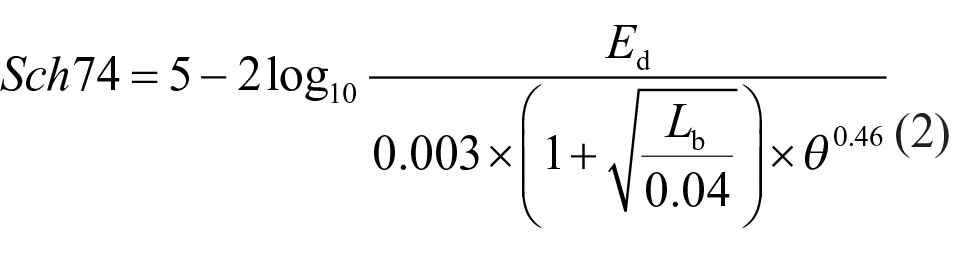
Consider next the model proposed by Schmidt-Clausen and Bindels for assessing discomfort glare from vehicle head lights.¹¹ Their data were obtained in a laboratory experiment that varied L_b, direct illuminance from source (E_d) and θ. Discomfort evaluations were given using a 9-point category rating scale, where subjects fixated on a test object and evaluated discomfort glare from a source that subtended 0.13° at the observer’s eye and was positioned at eccentricities ranging from 0.17° to 90° from central vision. The Schmidt-Clausen and Bindels’ model (Equation (2)), referred to as Sch74, uses the ratio of direct illuminance from the source and its background luminance. This model did not include a term for source size instead included a term for eccentricity from the point of visual fixation.

S c h 74 = 5 - 2 \log_{10} \frac{E_{d}}{0.003 \times (1 + \sqrt{\frac{L_{b}}{0.04}}) \times θ^{0.46}}

(2)

Petherbridge and Hopkinson⁹ examined the effect of source eccentricity and suggested that when visual tasks do not involve a fixed direction of view, it is preferable to neglect the effect of eccentricity up to 50°. They showed that for the same level of discomfort, source luminance was exponentially related to source eccentricity. This means that source luminance was proportionally related to 10^θ. Although modifications of source eccentricity up to 50° can affect the degree of perceived discomfort, such modifications were considered relatively insignificant, compared to modifications beyond 50°. For example, for the same source and background luminance, uncomfortable discomfort glare from a source at 5° eccentricity will only be reduced to ‘just acceptable’ at 50°, but discomfort will drop to ‘just imperceptible’ at 60° eccentricity. Petherbridge and Hopkinson’s model would be advantageous if the model is able to predict discomfort from glare in practical situations because a pedestrian’s gaze scans the whole environment and does not seem to fixate in a specific direction. This model does not require information about glare source position within the field of view, potentially making it easier to implement the design.

The Schmidt-Clausen and Bindels model, on the other hand, does not accommodate conditions with direct viewing of the source (θ = 0°), even though an approximation can be established by adopting a very small eccentricity in Equation (2).

Equations (1) and (2) both include background luminance. For pedestrians, it is unclear whether the luminance of a single surface, such as road surface, can be assumed to represent background luminance. In laboratory settings, it is possible to construct the visual field so that the background to the glare source is uniform and therefore relatively simple to characterize. In practical situations, such simplicities are unlikely: causes of non-uniformity include variations in background surfaces (such as traffic signs, trees and pavement materials) and luminance distribution is unlikely to be uniform. Such complexity makes it difficult to measure and characterize background luminance with one value. An alternative approach is to measure instead illuminance at the eye due to background.

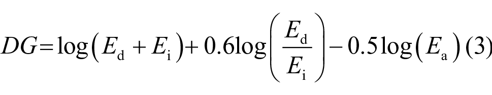
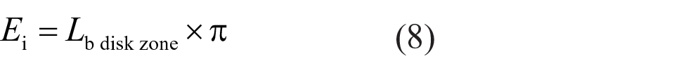
Bullough et al. developed a model for predicting discomfort using direct illuminance at the eye from source (E_d), indirect illuminance from source (E_i) and ambient illuminance (E_a).¹² Ambient illuminance is the illuminance at the eye from sources of light other than the glare source, as might be measured with the glare source switched off. The sum of these three illuminances is the total illuminance at the eye (E_t). In their work, E_d was measured using a baffle that blocked light surrounding the source, and E_a was measured when the source was switched off: to calculate E_i, the terms E_d and E_a were subtracted from E_t, as shown in Figure 1. To develop this model, Bullough et al. conducted a series of experiments in outdoor and indoor settings: they varied E_d, E_i and E_a and asked participants to look directly at the source and rate discomfort glare using a 9-point scale. Their proposed model shown in Equation (3) is used for calculating discomfort glare (DG), and Equation (4) is then used for transforming DG to a value on a 9-point De Boer-type scale (Bul08). This model did not include any measure of luminance nor the size nor position of the glare source, since observers were looking directly at the source.

Figure 1

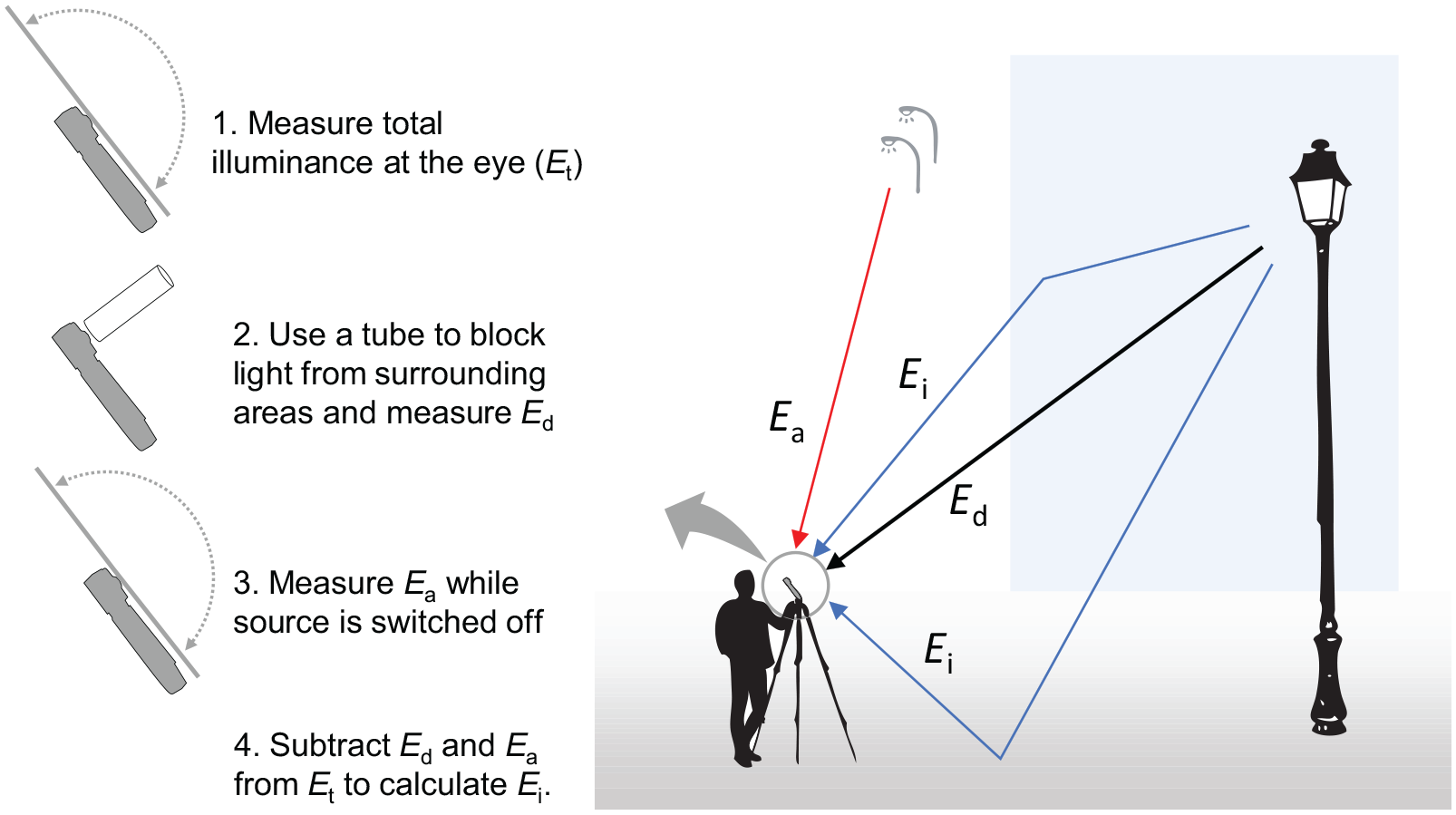
The three illuminance components used in Bul08 model (right) and the four steps needed to measure them (left)

In subsequent work, Bullough et al.¹⁴ concluded that maximum source luminance (L_max) was important for sources of size larger than 0.3° and hence added an additional term to their model (Equation (5)), referred to as Bul11, which transforms DG to a 9-point De Boer scale.

D G = \log (E_{d} + E_{i}) + 0.6 l o g (\frac{E_{d}}{E_{i}}) - 0.5 \log (E_{a})

(3)

B u l 08 = 6.6 - 6.4 \log D G

(4)

Bul 11 = 6.6 - 6.4 \log D G + 1.4 \log (\frac{50, 000}{L_{\max}})

(5)

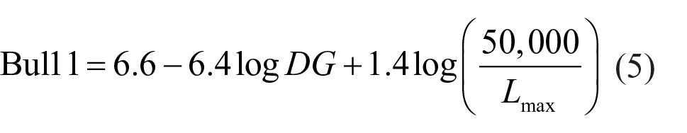
It is possible, however, that the results from the underlying study were confounded by effects of source size and luminance uniformity. Bullough¹⁵ used three sources that were generally larger than 0.3°: a bare LED array with maximum luminance (L_max) of 1 000 000 cd/m², the LED array covered with a plastic diffuser that produced L_max of 50 000 cd/m², and the same LED array but with the diffuser placed farther away from the LED array, producing L_max of 15 000 cd/m². For the same illuminance at the eye, a comparison between these three sources showed an effect of L_max on DG.

The term E_a in Equation (3) represents illuminance at the eye from sources of light other than the glare source, measured while the glare source is turned off. Precise measurement of this is not possible in the field, and instead, E_a must be defined by an assumed value: Bullough et al.¹² suggested values of 0.02 lx, 0.2 lx and 2 lx for very dark, suburban and urban districts, respectively.

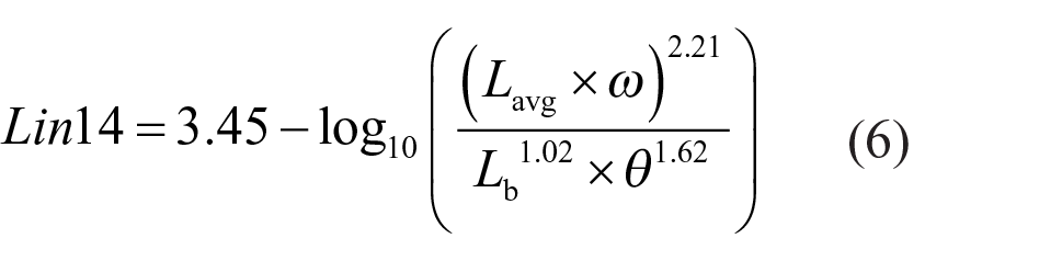
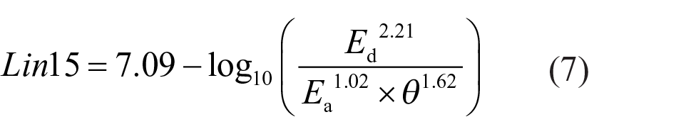
Lin and colleagues^10,13 proposed two models based on laboratory studies, one model being luminance based and one being illuminance based. Their first model (Lin14 shown in Equation (6)) is based on the contrast between L_avg and L_b. The study underlying this model found that E_d (as represented by the term L_avg × ω) was the most influential factor followed by L_b, then source eccentricity θ.¹⁰ Their second model (Lin15) includes illuminance from the source, ambient illuminance, as well as source eccentricity.¹³ In this later model, it is unclear whether their measurements of illuminance from source included only the direct component or both direct and indirect components. Because their use of illuminance from source was meant to replace the (L_avg × ω) term from Lin14, we assumed here that the Lin15 model refers to E_d (Equation (7)). Note that Lin14 and Lin15 have terms with similar exponents.

Lin15 was developed based on an experiment with varied E_d, E_a and θ and source-correlated colour temperature (CCT). Using a category rating procedure with a 9-point response scale, they found effects of illuminance from the source, E_a, and θ on DG ratings, but no effects of CCT.

Equation (7) was developed using a source that subtended 10° at the observer’s eye, but did not include a term for maximum source luminance as previously suggested by Bullough et al. for sources larger than 0.3°.¹⁴ Similar to the model of Schmidt-Clausen and Bindels (Equation (2)), Equation (7) uses eccentricity in the denominator, hence it yields an infinite value when directly looking at the source (i.e. when θ = 0°).

L i n 14 = 3.45 - \log_{10} (\frac{{(L_{avg} \times ω)}^{2.21}}{{L_{b}}^{1.02} \times θ^{1.62}})

(6)

L i n 15 = 7.09 - \log_{10} (\frac{{E_{d}}^{2.21}}{{E_{a}}^{1.02} \times θ^{1.62}})

(7)

The presented models result in predictions that are mapped to different scales, hence not all model predictions are comparable with each other. For example, low and high DG descriptors were mapped to Pet50 predictions in the range from 8 to 600, and to Sch74 predictions in the range from 3–7.^9,11 On the other hand, Bul08, Bul11, Lin14 and Lin15 provide predictions on a 1–9 De Boer scale.

Each of the models described above uses multiple variables to predict discomfort from glare – the luminance or illuminance from the source and its background, the size and/or location of the glare source relative to the observation point. However, they do not use the same variables: for example, Bullough et al. did not include any terms for source position because their experiments used on-axis viewing. In an experiment, the researcher’s decision to vary a certain parameter may lead to variation in the outcome measure, and hence to a conclusion that that parameter is important for discomfort from glare. Such a conclusion may not be correct: it depends on what other parameters were varied in the experiment and their relative degrees of prominence. This raises the question of which variables are essential for pedestrian application and considering practical constraints.

In outdoor environments after dark, pedestrians may experience discomfort from glare caused by street, path or public space lighting. The mounting height varies depending on lighting purpose; luminaires installed to illuminate paths and public spaces for pedestrians are mounted at shorter heights, for example, 3.7 m, and they are more closely spaced compared to street lighting.^16,17 Pedestrians scan the general environment to perform different tasks such as detecting trip hazards and identifying the intention and/or identity of an oncoming person.^18,19 This wide distribution in gaze directions means that a source of glare may appear at a wide range of locations in the visual field and at a wide range of distances and hence subtended sizes; the background field and the adaptation level will also vary.

While there is a broad range of possible scenes in which discomfort from glare is experienced, experimental work tends to consider only one or a small number of specific variations. This raises the question about the degree to which any such derived model, fitted precisely to those conditions, fits other situations: does precision in one context prevent sufficiency in broader contexts? In other words, is it possible to establish a simple model for discomfort which is satisfactory in most outdoor nighttime situations? One simple approach would be to characterize discomfort using E_d. This was considered in four studies^12,20–22 that generally found large (r > 0.5) correlations between E_d and subjective ratings of discomfort.²³ Similarly, it would be interesting to consider whether characterization of discomfort using only glare source luminance (e.g. L_avg or L_max) would be sufficient without the inclusion of a background luminance term to help define the contrast between light source and the background.

Authors will suggest their model to be useful if it successfully predicts the outcomes of the experiments from which it was developed. Success, usually indicated by an apparently high value of Pearson’s r or goodness of fit (R²), is not entirely surprising given the authors’ ability to adjust the constants and coefficients in their model to ensure that it gives a good fit. For a model to be generalizable to a broader range of applications, a better evaluation of success is the degree to which it predicts the outcomes of experiments carried out under a similar context but conducted by others. This was the approach taken in studies by Villa et al.²⁰ and Tyukhova and Waters.²⁴

Table 1 shows the reported correlations and goodness of fit for model predictions against DG ratings from their original data and also from independent data. This illustrates the importance of testing a model using independent data; for example, while Lin et al.¹⁰ reported r ⩾ 0.87 for their model, when that model was tested by Villa et al.²⁰ by using independent data, they reported a lower degree of association (Spearman’s rho = 0.38). The Villa et al. data suggest a better fit for other models. Table 2 shows correlations and goodness of fit for E_d and L_avg that were extended for pedestrian application. Several studies reported high correlations and goodness of fit for E_d and L_avg.

Table 1

Summary of reported Pearson’s r and Spearman’s rho correlation coefficients, and goodness of fit (R²) for pedestrian context models

Model	Reported performance in model development study	Tyukhova and Waters²⁴ (n = 1692)	Villa et al.^{20 †} (n = 1056)
Pet50 (Equation (1))	Not reported	–	–
Sch74 (Equation (2))	Not reported	r = 0.79^§	rho = 0.75^§
Bul08 (Equation (4))	R² = 0.70^§ (n = 796)	r = 0.86^§ for predictions from Bul08 and Bul11	–
Bul11 (Equation (5))	Not reported	r = 0.86^§ for predictions from Bul08 and Bul11	–
Lin14 (Equation (6))	r = 0.87^§ for 3000 K source (n = 168); r ⩾0.95^§ for 5000 K (n = 54) and 6500 K (n=80) sources	–	rho = 0.37^§
Lin15 (Equation (7))	R² = 0.96 for young subjects (n = 960), R² = 0.88 for seniors (n = 240)	–	rho = 0.75^§

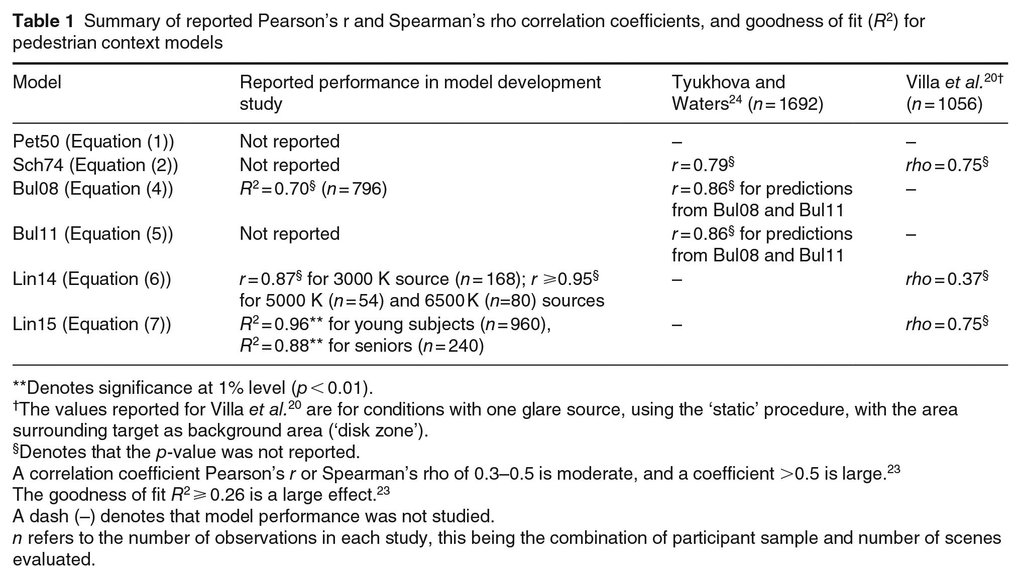
Denotes significance at 1% level (p < 0.01).

†

The values reported for Villa et al.²⁰ are for conditions with one glare source, using the ‘static’ procedure, with the area surrounding target as background area (‘disk zone’).

Denotes that the p-value was not reported.

A correlation coefficient Pearson’s r or Spearman’s rho of 0.3–0.5 is moderate, and a coefficient >0.5 is large.²³

The goodness of fit R² ⩾ 0.26 is a large effect.²³

A dash (–) denotes that model performance was not studied.

n refers to the number of observations in each study, this being the combination of participant sample and number of scenes evaluated.

Table 2

Summary of reported Spearman’s rho and goodness of fit (R²) for simple models that may be extended for pedestrian application

Model	Villa et al.^{20 †} (n = 1056)	Kohko et al.²¹ (n = 1617)	Sivak et al.²² (n = 400)	Bullough et al.¹² (n = 796)^‡
E _d	rho = 0.72^§	R² = 0.70^§ for central; R²= 0.53^§ for peripheral viewing	R² = 0.99**	R² = 0.93^§ (exp 2), 0.73^§ (exp 5), and 0.45^§ (in/out exp)
L _avg	rho = 0.74^§	R² = 0.80^§, 0.81^§ for central and peripheral viewing	–	R² = 0.02^§ (exp 2)

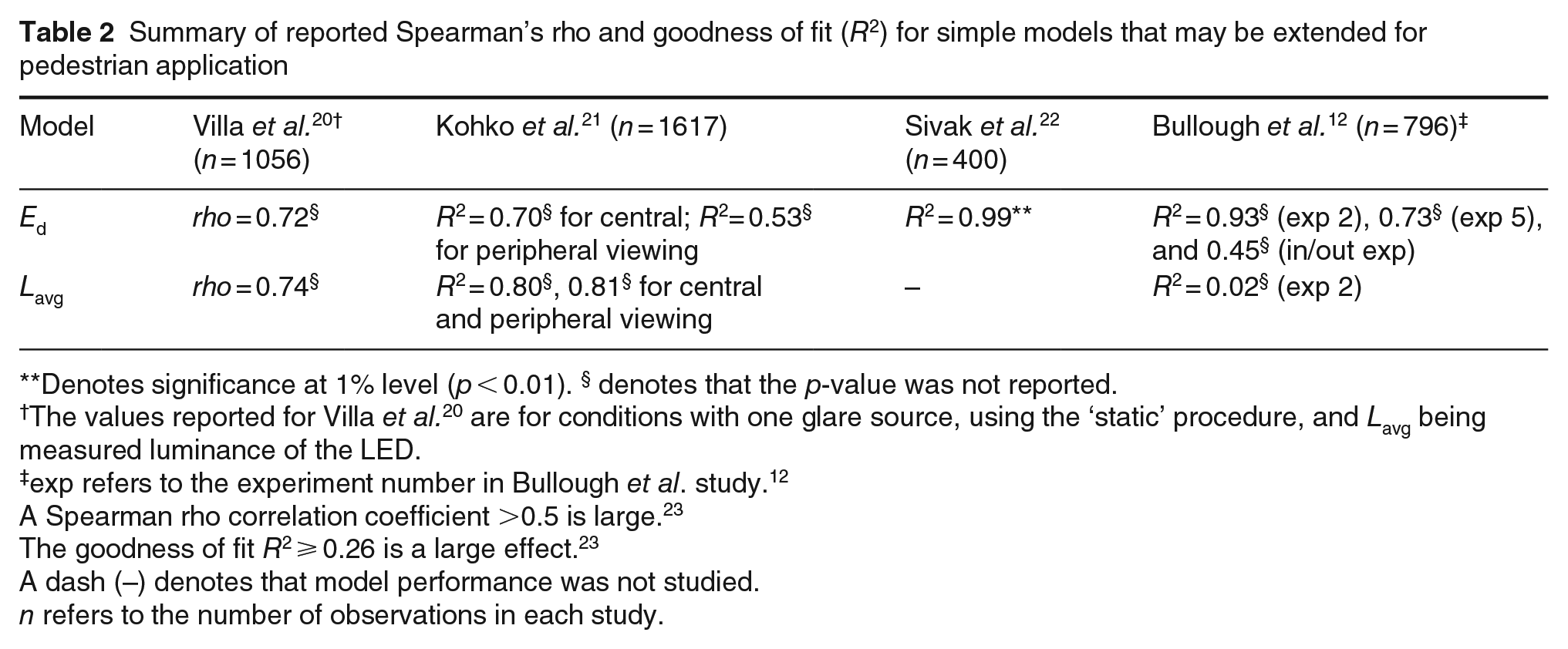
Denotes significance at 1% level (p < 0.01). ^§ denotes that the p-value was not reported.

†

The values reported for Villa et al.²⁰ are for conditions with one glare source, using the ‘static’ procedure, and L_avg being measured luminance of the LED.

‡

exp refers to the experiment number in Bullough et al. study.¹²

A Spearman rho correlation coefficient >0.5 is large.²³

The goodness of fit R² ⩾ 0.26 is a large effect.²³

A dash (–) denotes that model performance was not studied.

n refers to the number of observations in each study.

It can be problematic to draw conclusions about model performance using only the results of one study. A certain dataset may have inadvertently favoured one model due to the context or the range of lighting conditions used in that experiment. To provide a more exhaustive analysis, we follow the comparison of models for predicting discomfort from daylight as reported by Wienold et al.²⁵ In that study they compared the predictions of 22 models using seven datasets, comparing the performance of different models using diagnostic tests based on receiver operating characteristic (ROC) curve characteristics such as true positive rate, true negative rate, area under the curve and squared distance.

The current work investigated the performance of seven models for predicting discomfort from glare in an outdoor context using four independent datasets. These were five previously proposed multi-term models (Equations (1), (2), (4), (6) and (7)) and two one-term models (the quantities E_d and L_avg).

2. Method

2.1 Evaluated models

The evaluated models include Pet50, Sch74, Bul08, Lin14, Lin 15, E_d and L_avg. The intent was also to include the Bul11 model, but as discussed below in Section ‘Included studies and datasets’, not all datasets reported maximum luminance as needed in that model, and hence it was not possible to include it.

2.2 Study and data inclusion criteria

A search was conducted to identify experimental studies of discomfort from glare having relevance to lighting conditions experienced by pedestrians. These conditions include low levels of luminance adaptation, a wide range of source eccentricities and a wide range of source sizes that can result from combinations of different eccentricities and distances from source. The search was conducted using common keywords: ‘discomfort glare’, ‘nighttime’ and ‘pedestrians’ and only peer-reviewed journal articles written in English were retained. These articles were reviewed, and study parameters were evaluated according to inclusion criteria:

Lighting conditions should include a dark background representative of nighttime environments.

Only one light source. This criterion was used to isolate and omit effects related to multiple light sources and the different approaches that may be used.²⁶

Only data related to white sources. Coloured sources were not included.

Where relevant, viewing distance or mounting height low enough to mimic pedestrians viewing conditions.

Test participants were stationary (standing still or sitting) whilst observing and evaluating the scene. Dynamic viewing protocols, where subjects walked on a specified path then provided a rating, were not considered.

Details of the visual scene including average luminance of source, background luminance, direct, indirect, and ambient illuminances, source size, and eccentricity were reported.

During trials, presentation order of lighting conditions was randomized to offset order bias.

Experimental data were independent of the models evaluated in the current work.

The authors responded to our request to provide experimental data.

We do not consider the impacts of multiple sources and dynamic viewing to be unimportant. They were excluded here to simplify the analysis because it is unclear how the seven models can be used with more than one glare source. For ratings collected using a dynamic viewing procedure, it is unclear which viewing position parameters, for example, eccentricity, to use in the models: that again suggests an advantage of predicting discomfort using a simplified measure such as E_d.

2.3 Included studies and datasets

The search identified eleven relevant studies. Four studies were not included because they did not report required quantities such as L_avg^22,27,28 or did not randomize the presentation order of lighting conditions.²¹ Other studies were not included either because our attempts to contact those authors were unsuccessful or those data were not independent of the current analysis, having been used to develop a model assessed in the current analysis.^10,12,13 Four studies met the inclusion criteria: in all four cases, those authors responded to our requests to provide study data.^20,24,29,30 Not all four studies measured and reported maximum luminance, hence Bul11 (Equation (5)) was not evaluated.

The first dataset was from a study conducted by Villa et al.²⁰ in an outdoor test track. Here we use the data from their 32 conditions (4 luminaire types × 4 distances from luminaire × 2 view directions) with one source of glare observed from a stationary location and ignore data from their trials with either two sources of glare and/or dynamic viewing. This dataset is referred as V17. The 33 test participants were asked to rate each lighting condition using a 9-point scale. Villa et al. used high dynamic range images to establish two background luminance measurements: the first measurement was based on a circle with 30° diameter surrounding the visual target (named by the authors as ‘disk zone’); whereas the second measurement was based on a rectangular area that included the two viewing targets and the road surface. In the current analysis, we used the disk zone measurement, given that both measurements yielded similar results in their analysis. To calculate E_i, L_b of the disk zone area was converted using Equation (8) assuming a Lambertian distribution.

E_{i} = L_{b disk zone} \times π

(8)

The second dataset from Sweater-Hickcox et al.,²⁹ named as S13, included data from their three experiments that were conducted in a laboratory room. Conditions related to the white LED array with a white surround were included (13 lighting conditions). Conditions where the LED array had yellow or blue surround were not included because these conditions were ineligible according to the criteria in ‘Study and data inclusion criteria’. Conditions with a dark surround were not included because information about the LED source size was not available. In the first experiment, ten participants sat 3 m away from the LED array and rated DG at four levels of E_d, whereas in the second experiment eight participants repeated this procedure while being seated 6 m away from the LED array. In the third experiment, the source size was decreased, and the procedure was repeated with six participants seated 3 m away. Each participant rated the same lighting condition three times using a 9-point scale, and the mean of these three ratings was used in the current analysis as was done in the published study.

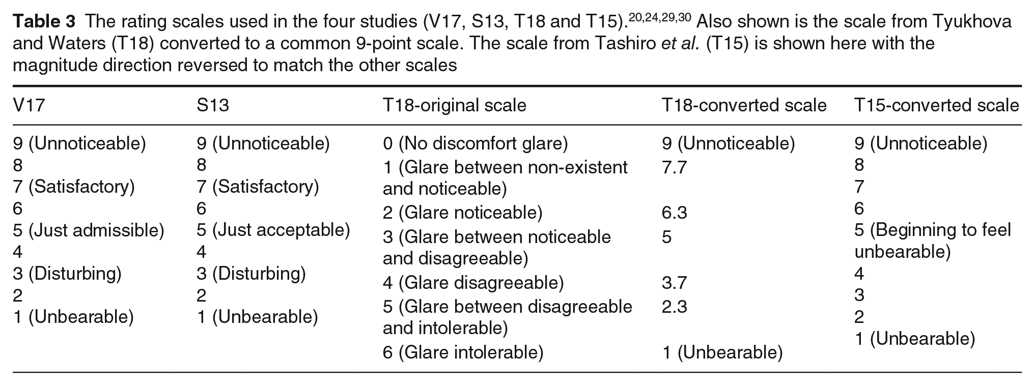
The third dataset, from Tyukhova and Waters,^24,31 named here as T18, examined small bright sources (subtending 0.0001 sr and 0.00001 sr at the observer’s eyes) and included 36 lighting conditions (3 levels of L_avg × 2 eccentricities × 2 source sizes × 3 levels of L_b) which were rated by 47 test participants. This was a laboratory experiment with participants seated in a spherical apparatus. Evaluations of discomfort were given using a 7-point scale: for the current analysis, these were transformed to a 9-point scale by mapping the end points of the original scale from 0 (No discomfort glare) and 6 (Glare intolerable) to 9 (Unnoticeable) and 1 (Unbearable),³² respectively, with equal incremental steps. The transformation between scales, shown in Table 3, was necessary for the analysis of a combined dataset described in Section 2.4. This conversion assumed that participants linearly map their responses to the range of the scale presented. This scale transformation meant that ratings in the three studies were along similar response scales.

Table 3

The rating scales used in the four studies (V17, S13, T18 and T15).^20,24,29,30 Also shown is the scale from Tyukhova and Waters (T18) converted to a common 9-point scale. The scale from Tashiro et al. (T15) is shown here with the magnitude direction reversed to match the other scales

V17	S13	T18-original scale	T18-converted scale	T15-converted scale
9 (Unnoticeable) 8 7 (Satisfactory) 6 5 (Just admissible) 4 3 (Disturbing) 2 1 (Unbearable)	9 (Unnoticeable) 8 7 (Satisfactory) 6 5 (Just acceptable) 4 3 (Disturbing) 2 1 (Unbearable)	0 (No discomfort glare)	9 (Unnoticeable)	9 (Unnoticeable) 8 7 6 5 (Beginning to feel unbearable) 4 3 2 1 (Unbearable)
		1 (Glare between non-existent and noticeable)	7.7
		2 (Glare noticeable)	6.3
		3 (Glare between noticeable and disagreeable)	5
		4 (Glare disagreeable)	3.7
		5 (Glare between disagreeable and intolerable)	2.3
		6 (Glare intolerable)	1 (Unbearable)

The fourth dataset from Tashiro et al.,³⁰ named here as T15, examined sources with different LED arrangements, intensity levels and background luminances (17 sources × 7 intensity levels × 3 background luminances) that were rated by 8, 12, 19 and 11 participants in four experiments conducted in a laboratory room. This dataset (labelled here as T15) initially included ratings on a 9-point scale where points 1, 5 and 9 corresponded to unnoticeable, beginning to feel unbearable and unbearable levels of discomfort, respectively. This scale was reversed to align with the magnitude direction used in the other datasets. Tashiro et al. study did not measure E_d, E_i and E_a, but because the experiment apparatus was surrounded by a black curtain of low reflectance (~3%), we assumed that E_i is negligible = 0.0001 lx. At the lowest background luminance level of 0.1 cd/m², we also assumed that E_a is negligible = 0.0001 lx. At the other two background luminance levels (1 cd/m² and 10 cd/m²), E_a was calculated for each source by subtracting total illuminance at the lowest source intensity under 0.1 cd/m² from corresponding total illuminance under 1 cd/m² and 10 cd/m². This yielded an ambient illuminance value for each source that was used for all intensities.

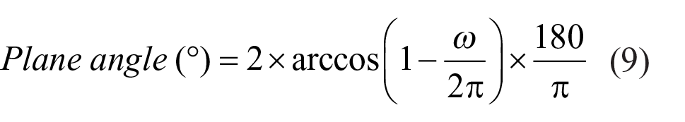
The four datasets included a wide range of E_d as shown in Table 4. Indirect illuminance and illuminance from other light sources were small (<4 lx) representing a dark background. Given that Bul08 model was suggested for sources <0.3°, we also show in Table 4 source sizes in plane degrees for each dataset. The conversion from steradians to degrees was done using Equation (9) assuming a conical solid angle.³³

P l a n e a n g l e (°) = 2 \times \arccos (1 - \frac{ω}{2 π}) \times \frac{180}{π}

(9)

Table 4

Summary of the experimental conditions in the four datasets

Parameter	Dataset
Parameter	V17	S13	T18	T15
Number of participants	33	10; 8; 6	47	8; 12; 19; 11
Number of experimental conditions	32	5; 5; 3	36	63; 168; 63; 63
Number of observations	1056	108	1692	4410
Number of observations with ratings < 5	99	74	846	1836
Number of observations with ratings ⩾ 5	957	34	846	2574
E_d (lx)	4.2–25.2	4.7–15.0	0.2–81.5	0.02–92.3
E_i (lx)	0.11–0.74	0	0.02–0.06	0
E_a (lx)	0.05–0.09	0.2	0.11–3.58	0–0.95
L_avg (cd/m²)	11 000–152 000	401–1041^†	20 477–766 440	1.56–177 617
L_b (cd/m²)	0.034–0.237	0	0.037-1.156	0.1; 1; 10
Eccentricity (°)	23–62	0	0; 10	8.5
Source size (sr)	0.00044–0.00823	0.00096; 0.00383	0.00001; 0.0001	0.0001–0.0081
Source size (°)	1.36–5.87	2; 4	0.2; 0.65	0.65–5.82

†

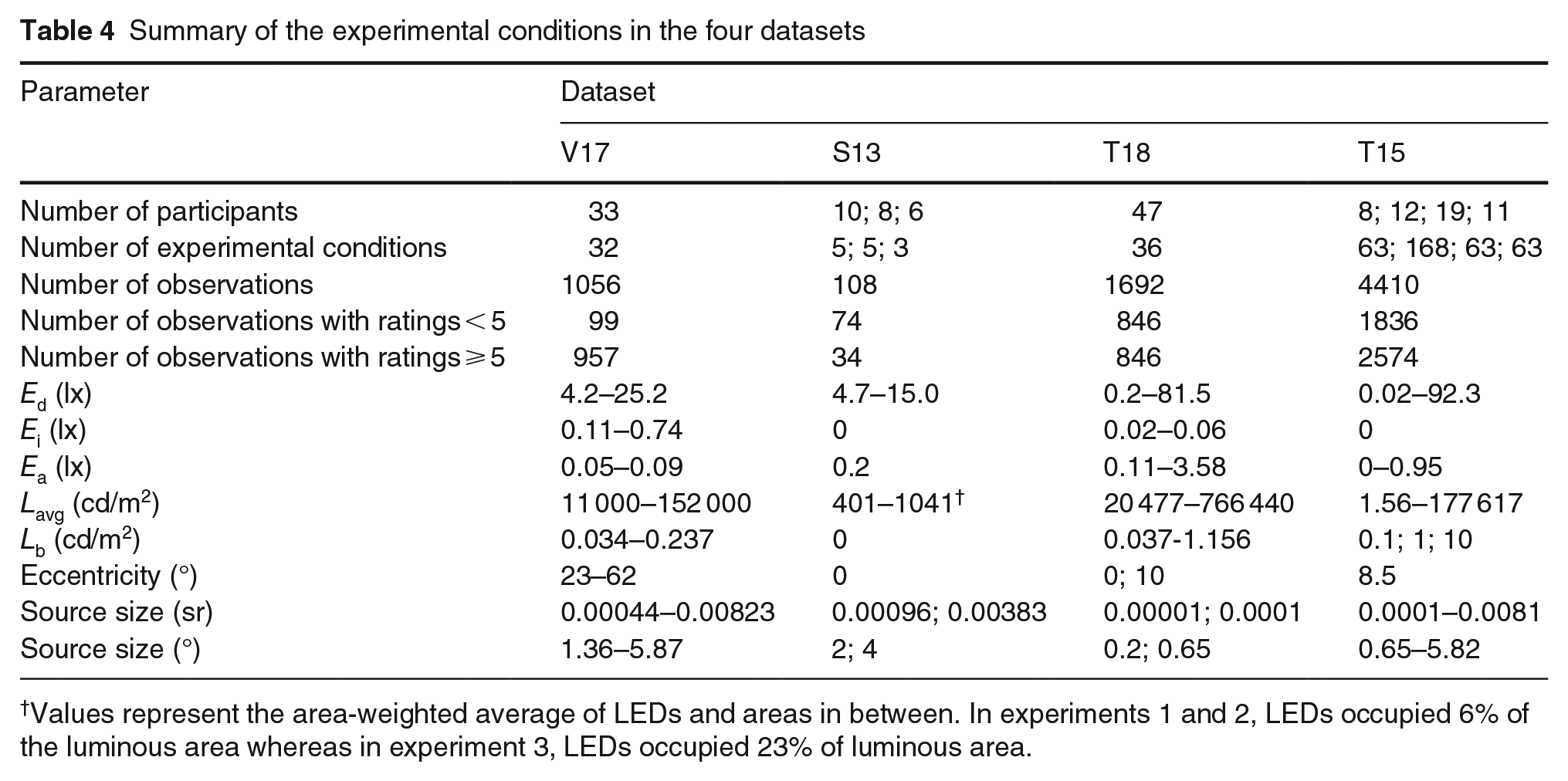
Values represent the area-weighted average of LEDs and areas in between. In experiments 1 and 2, LEDs occupied 6% of the luminous area whereas in experiment 3, LEDs occupied 23% of luminous area.

2.4 Model performance evaluation

Models of discomfort from glare were tested by using them to predict the outcome of previous work (the datasets defined in Section ‘Included studies and datasets’) and comparing those predictions with the results of each experiment. The relative performance of each model was established using a range of statistical tests following the example of Wienold et al.²⁵

In order for a DG model to be useful for pedestrian applications, model performance can be judged based on two criteria: (1) the degree of correlation between model predictions and evaluation responses from test participants; and (2) the ability to distinguish between discomfort and non-discomfort situations. The models were expected to provide a relative – not absolute – indication of glare. Hence, evaluations based on absolute model values such as root mean square error and the consistency of borderline between comfort and discomfort (BCD) were not considered.

The degree of association was assessed using Spearman rank correlation rho, a nonparametric test that determines the degree to which a monotonic relationship exists between two sets of ranks.³⁴ A rho value 0–0.1 is considered very small, 0.1–0.3 is small, 0.3–0.5 is moderate, ⩾0.5 is large.²³

The p-values of these Spearman correlations were compared to the Holm’s sequential Bonferroni thresholds, which provides protection against type I error.³⁵ This method orders the p-values from smallest to largest and uses progressively less stringent significance thresholds based on the number of remaining tests (α/k, α/(k-1), α/(k-2), etc. where k is the number of tests and α is the significance level).

To determine how well each model was able to distinguish between discomfort and non-discomfort situations, four tests were employed as shown in Figure 2.

– True negative rate (TNR), also known as specificity, describes the ability of a model to accurately detect non-DG (subjective rating ⩾5).

– True positive rate (TPR), also known as sensitivity. TPR describes the ability of a model to accurately detect the presence of discomfort (subjective rating <5).

– Area under the curve (AUC) describes the diagnostic accuracy of a model: suggested thresholds for describing diagnostic accuracy are AUC 0.5 to 0.6 = fail, 0.6–0.7 = poor, 0.7–0.8 = fair, 0.8–0.9 = good and 0.9–1 = excellent.³⁶

– Squared distance (SqD) is the square of the distance between the point of ideal performance (TPR = 1, TNR = 1) and any point on the ROC curve. The point on the curve closest to the upper left corner (smallest SqD) is considered an optimal cut-off point for balancing TPR and TNR.^37,38 In this analysis, we use 1-SqD instead of SqD so that a larger value is better, matching interpretation of TNR, TPR and AUC.

The mean of TNR, TPR, AUC and 1-SqD was calculated to provide an indication of overall performance. This mean value is between 0 and 1 where a higher value indicates a better performance. We used the mean performance, rather than rank orders based on individual performance scores as was used in a previous work²⁵ because this preserves the magnitude of differences between model performances. A difference in rank order of 1.0 would be given to two models regardless of whether the difference in their performance scores was large or small.

Figure 2

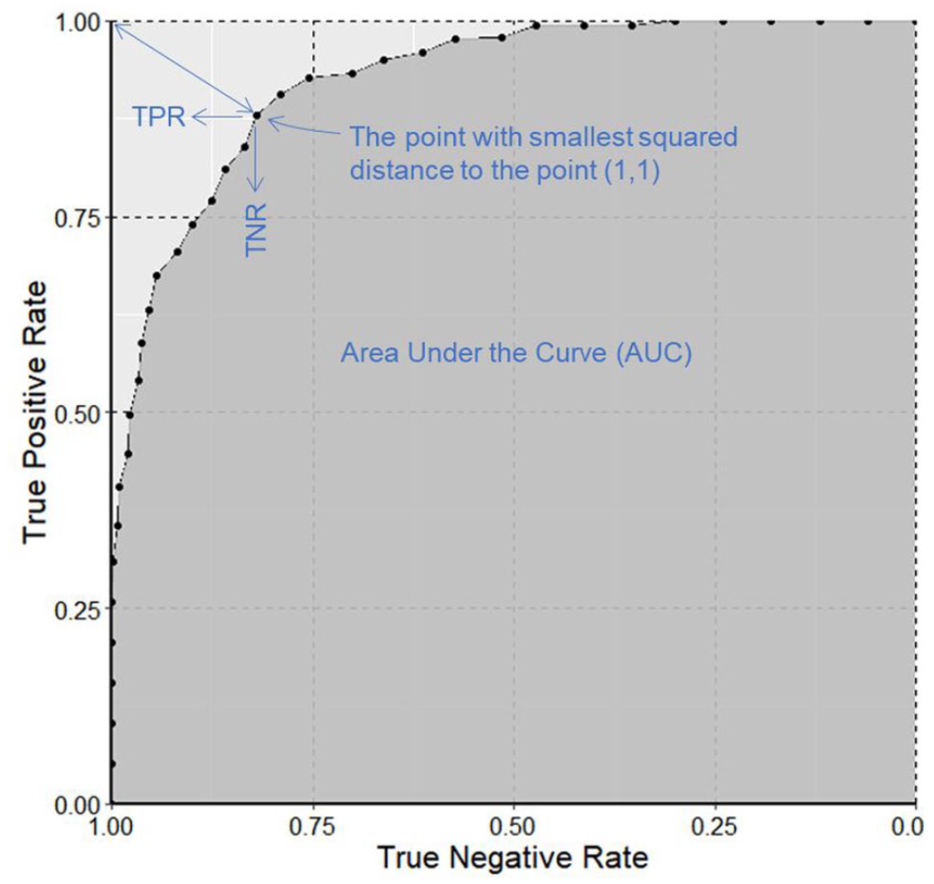
An example ROC plot showing the point with smallest squared distance to the point (1, 1) and corresponding TNR and TPR. The darker shaded area represents AUC

The data used for evaluation of the seven models were at the subject level, that is, lighting conditions and responses for each test participant were used as opposed to using grouped data such as mean ratings from a group of test participants for a certain lighting condition. This was done to uncover the uncertainty inherent in DG studies.³⁹

The analyses used here (except for Spearman correlations) required that ratings were converted from a 9-point scale to binary evaluations of whether or not there was discomfort. This was done by assuming that ratings of less than 5 (just acceptable/admissible, the centre of the 9-point scale) were considered to cause discomfort, while ratings of 5 or greater were considered indicating no discomfort. Our assumption of using the centre of the scale is similar to the assumption made by Wienold et al.²⁵ where a 4-point scale was split in half and converted into a binary variable. Lin and others also found when 50% of participants were comfortable, the borderline between comfort and discomfort corresponded to 4.7 on the 9-point rating scale.¹⁰ This aligns with the definition of borderline BCD at point 5 on a 9-point scale.⁴⁰

Analyses were conducted using R Studio (version 3.6.3) and the ROCR package.⁴¹ Model performances were analysed for the four datasets combined and then for each dataset individually.

2.5 Assumptions

A few assumptions were required to calculate the seven models. First, Pet50 was applied to all eccentricities including two eccentricities above 50° in V17 dataset. Although this model was suggested for eccentricities up to 50°, we implemented the model using all datasets including two eccentricities (out of eight eccentricities tested) higher than 50° in the V17 dataset. The reason it was implemented even for cases higher than 50° in our analysis is because we were interested in evaluating the model relative to other models. If it performs well, it would be helpful for pedestrian applications, given that a specific eccentricity cannot be assumed.

Second, to avoid infinite values resulting from zeros in the denominator or in logarithms, these zeros were replaced with a very small value (e.g. 0.0001 lx). This occurred in three cases: (1) because E_i and E_a were assumed to be negligible in T15 dataset as described in Section ‘Included studies and datasets’, which would result in a zero in the denominator in Bul08; (2) when calculating Lin14 and Lin15 for viewing conditions with an eccentricity of zero as in S13 and T18 datasets; and (3) when calculating Pet50 or Lin14 for conditions with negligible L_b as in S13 dataset.

Third, in Lin15, it is unclear whether their measured illuminance from the glare source includes both direct and indirect components or only the direct component. In this analysis, we assumed that their illuminance measurements from glare source are represented with E_d as shown in Equation (7).

3. Results

Figure 3 shows the mean of four diagnostic tests (TNR, TPR, AUC and 1-SqD) using the combined dataset: results for the individual tests are shown in Figure 4. Table 5 shows results for each test using combined and individual datasets.

Figure 3

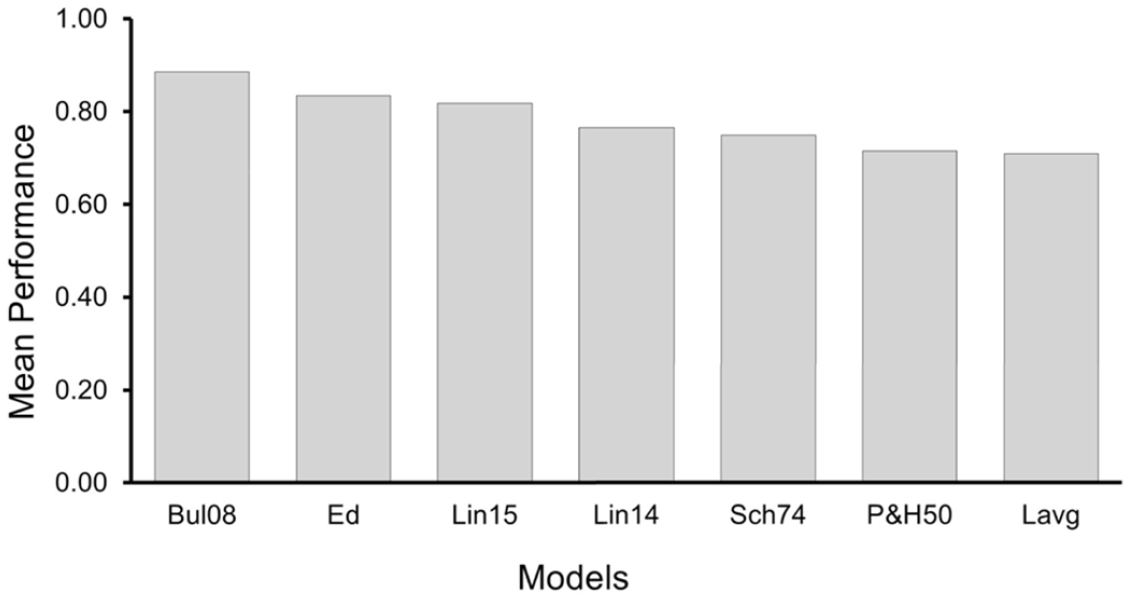
Mean of the diagnostic tests (TNR, TPR, AUC and 1-SqD) for the seven models using the combined dataset. A higher mean value indicates a better performance

Figure 4

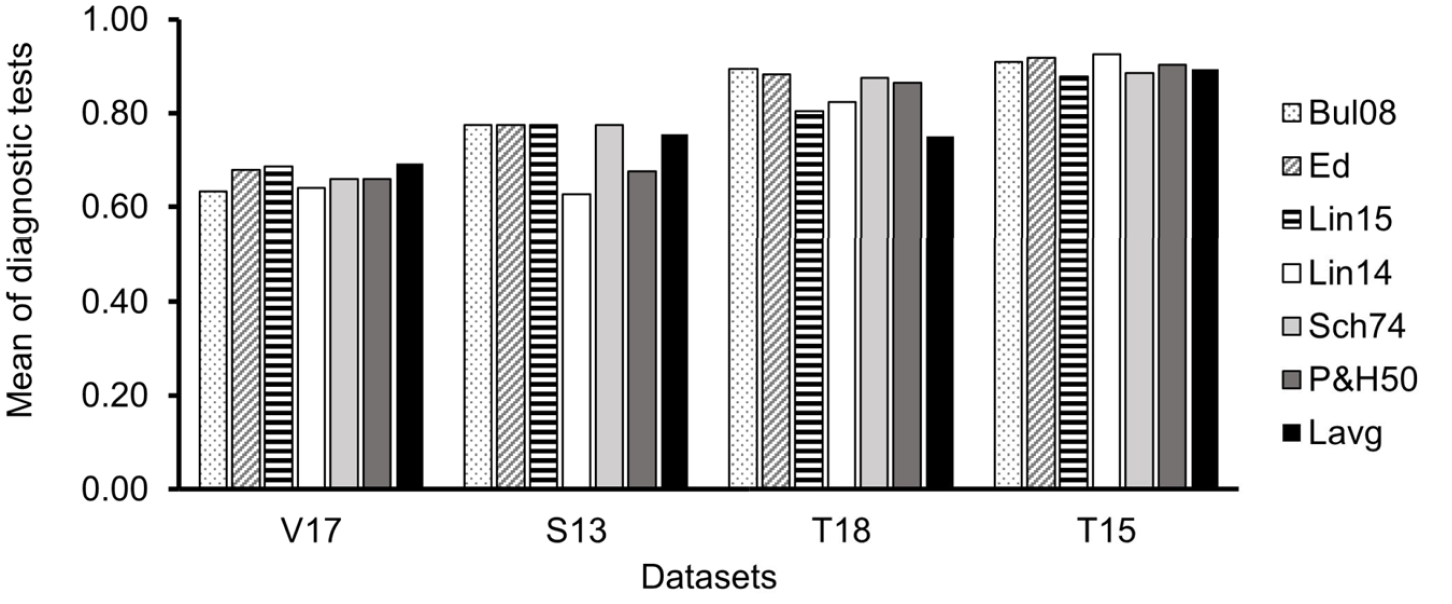
Mean of five diagnostic tests (TNR, TPR, AUC and 1-SqD) for the seven models using individual datasets. A higher mean value indicates a better performance

Table 5

Diagnostic test results based on each dataset as well as the combined dataset

Dataset	Model	TNR	TPR	AUC	1-SqD	Mean^§	Spearman rho
V17	E _d	0.66	0.64	0.67	0.75	0.68	−0.27**
	L _avg	0.67	0.66	0.67	0.77	0.69	−0.25**
	Lin14	0.59	0.65	0.62	0.71	0.64	0.21**
	Lin15	0.61	0.69	0.69	0.75	0.69	0.29**
	Bul08	0.63	0.58	0.63	0.69	0.63	0.22**
	Pet50	0.62	0.65	0.63	0.73	0.66	−0.22**
	Sch74	0.58	0.68	0.66	0.72	0.66	−0.25**
S13	E _d	0.80	0.67	0.78	0.85	0.78	−0.49**
	L _avg	0.82	0.63	0.75	0.83	0.75	−0.51**
	Lin14	0.73	0.48	0.64	0.66	0.63	0.21^NS
	Lin15	0.67	0.80	0.78	0.85	0.78	0.49**
	Bul08	0.67	0.80	0.78	0.85	0.78	0.49**
	Pet50	0.75	0.55	0.68	0.73	0.68	−0.28*
	Sch74	0.67	0.80	0.78	0.85	0.78	−0.49**
T18	E _d	0.81	0.86	0.91	0.94	0.88	−0.8**
	L _avg	0.68	0.71	0.78	0.82	0.75	−0.54**
	Lin14	0.76	0.78	0.86	0.89	0.82	0.7**
	Lin15	0.69	0.81	0.85	0.87	0.80	0.69**
	Bul08	0.82	0.88	0.93	0.95	0.89	0.82**
	Pet50	0.75	0.91	0.88	0.93	0.87	−0.74**
	Sch74	0.83	0.83	0.91	0.94	0.88	−0.8**
T15	E _d	0.86	0.89	0.95	0.97	0.92	−0.86**
	L _avg	0.83	0.88	0.92	0.95	0.89	−0.81**
	Lin14	0.89	0.89	0.95	0.97	0.93	0.88**
	Lin15	0.81	0.86	0.90	0.94	0.88	0.78**
	Bul08	0.89	0.85	0.94	0.97	0.91	0.84**
	Pet50	0.86	0.86	0.93	0.96	0.90	−0.84**
	Sch74	0.88	0.81	0.91	0.95	0.89	−0.79**
Combined data set	E _d	0.78	0.79	0.86	0.91	0.83	−0.69**
	L _avg	0.55	0.82	0.70	0.76	0.71	−0.45**
	Lin14	0.84	0.63	0.75	0.84	0.76	0.54**
	Lin15	0.81	0.73	0.84	0.89	0.82	0.68**
	Bul08	0.84	0.84	0.91	0.95	0.88	0.78**
	Pet50	0.58	0.79	0.71	0.78	0.72	−0.47**
	Sch74	0.74	0.66	0.78	0.82	0.75	−0.58**

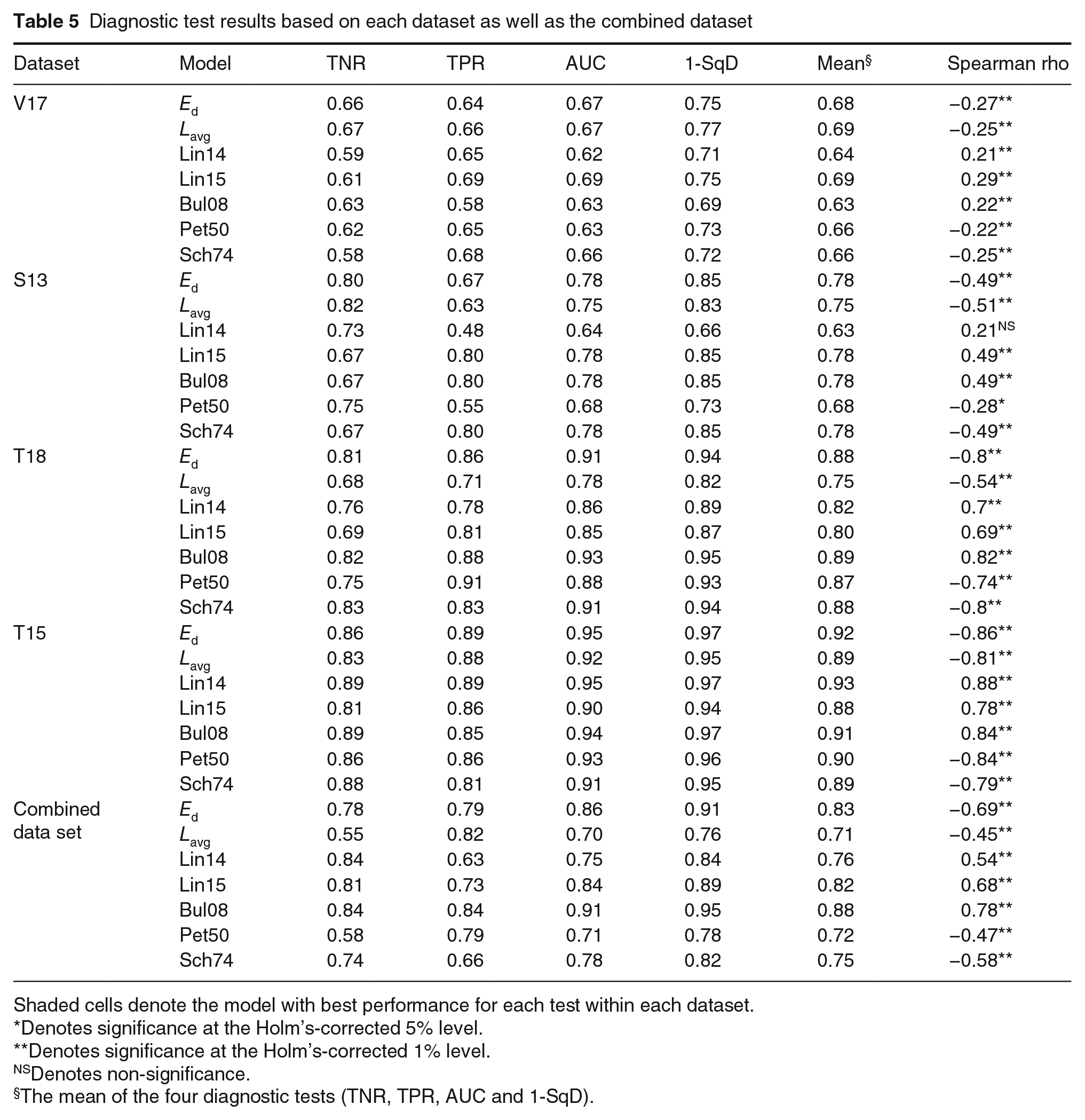
Shaded cells denote the model with best performance for each test within each dataset.

Denotes significance at the Holm’s-corrected 5% level.

Denotes significance at the Holm’s-corrected 1% level.

Denotes non-significance.

The mean of the four diagnostic tests (TNR, TPR, AUC and 1-SqD).

For the combined data set, the highest mean performance was found for Bul08, followed by E_d and Lin15, and the lowest scores were for L_avg and Pet50. The differences were, however, small, and in all cases the mean test performance was above 0.7. AUC values suggested an excellent performance for Bul08 and a good performance for E_d and Lin15. On the other hand, L_avg and Pet50 had lowest mean performance, and AUC values suggested only a fair performance (Table 5). Spearman’s rho ranged from 0.45 to 0.78 and these values were suggested to be statistically significant for all models.

Results of analyses using individual datasets varied and did not fully match results from the combined dataset (Figure 4, Table 5). Bul08 had the highest mean performance only for one dataset (T18) and was tied with other models using S13 dataset. In another dataset (V17), L_avg and Lin15 had a higher mean performance than Bul08. Lin15 had lowest mean performance using T15 dataset. Differences between models varied by dataset. With the V17 and T15 datasets, each model gives a similar mean performance; with S13 and T18 there is a wider range of mean performance scores.

AUC was found to be greater than 0.6 for all models using the individual data sets, indicating that no models failed. There was, however, a difference in AUC ranges between data sets; all models had a poor performance (AUC 0.6 to 0.7) using V17 but an excellent performance (AUC > 0.9) using T15. Using S13, AUC values suggested a poor performance for Lin14 and Pet50. For T18, Bul08, E_d and Sch74 had an excellent performance.

For all models, Spearman’s correlations were small and statistically significant using V17, mostly moderate and significant using S13, and large and significant using T18 and T15. Detailed graphs of diagnostic test results and Spearman correlations for each model are included in Appendix A.

4. Discussion

4.1 Combined dataset

Consider first the performance of models using the combined data set, this being the wider range of lighting conditions and thus a better analysis of applicability in practice. The best performance was obtained with Bul08, this model having the highest mean test score, including an AUC of 0.91, and the highest Spearman rho. The next best performance was given by E_d, this having the second highest mean test score, AUC and Spearman’s rho. The improved performance of Bul08 over E_d might be due to the contrast term (E_d/E_i) which helps differentiate between situations that had the same influence of saturation, as is characterized by E_d, but with different indirect illuminances and hence different source to background contrast.

Lin15 performed only slightly less well than did E_d, having the third highest mean test score and Spearman’s rho. One feature of these three models (Bul08, E_d and Lin15) is that they characterize source brightness using illuminance rather than luminance. L_avg, on the other hand, provided the lowest mean test score and Spearman’s rho of all models, although the AUC being 0.7 indicates that L_avg still had a fair performance. This is in line with Bullough et al. who reported that L_avg had lower association with DG ratings than did E_d as shown in Table 2.¹²

The use of Bul08 or Lin15 would be challenging in field evaluations where the source cannot be switched off to measure E_a. For Bul08, Bullough et al.¹² suggested using typical values (0.02 lx, 0.2 lx and 2 lx for very dark, suburban and urban districts, respectively) but these may not match actual conditions: error within these assumptions may contribute to increased variance in the model performance. Compared to Bul08, another complication for using Lin15 in field evaluation is the need to make an assumption of eccentricity.

E_d, a single measurement of illuminance, gives a similar performance to Bul08 and Lin15, despite those being more complex models which include multiple factors. This result holds even if one of the datasets is removed (see further analysis in Appendix B). Log(E_d) returns the same diagnostic test results as E_d and might be preferred over E_d due to its linear relationship with DG responses. E_d, on the other hand, exhibits a decreasing exponential relationship with DG ratings.

4.2 Individual datasets

Analyses using the combined dataset reveal the order in which the models more accurately predict the discomfort data (Figure 3). When the datasets are considered individually, however, this order is not retained in any individual dataset, although the differences between models in many cases are small. In other words, certain datasets favour certain models. Bul08, the model which performs best for the combined dataset, also performs well for S13, T15 and T18 but performs less well than other models for V17. Given that Bul08 was developed with direct viewing, the reduced performance of Bul08 using V17 might be due to the larger eccentricities used in V17 compared to those in S13, T18 and T15.

On the other hand, E_d tends to be one of the better performing models for each of the four datasets. While analyses using the combined dataset suggested that L_avg gave the weakest performance, Figure 4 shows that it performs similar to the other models for three datasets (V17, S13 and T15) and drops to the weakest performance only for T18.

The performance of L_avg using T18 might have been affected by experimental conditions because this dataset included two source sizes that had the same L_avg but the larger source, expectedly, caused higher discomfort. For instance, for all experimental conditions, the mean DG rating was 3.3 for the larger source compared to 5.9 for the smaller source. Lin14 and Pet50 had a better performance than L_avg in T18 dataset as they both account for source size.

Bullough et al. suggested that the Bul08 model be used with sources subtending a size at the observer of smaller than 0.3°.¹⁴ For sources larger than 0.3° they proposed Bul11, a model which also includes maximum luminance. To evaluate whether Bul08 performance in the current analyses might be further enhanced if only used with sources smaller than 0.3°, we used T18 dataset where half of the cases had a source size of 0.2° and the other half was 0.65°. Contrary to the proposal to use Bul08 for sources smaller than 0.3°, we found that Bul08 performed similarly well regardless of whether the source size was 0.2° or 0.65° (Table 6).

Table 6

Analysis results of Bul08 model using T18 dataset broken down by source size

Source size	TNR	TPR	AUC	1-SqD	Spearman Rho	Mean^§
0.2°	0.912	0.704	0.871	0.905	0.705**	0.85
0.65°	0.903	0.846	0.924	0.9671	0.762**	0.91

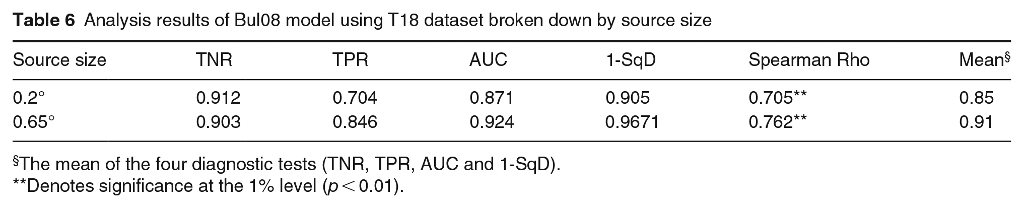
The mean of the four diagnostic tests (TNR, TPR, AUC and 1-SqD).

Denotes significance at the 1% level (p < 0.01).

In contrast to T18 dataset, V17 works slightly better with L_avg than Bul08. In V17, variations in L_avg were affected by participant’s position and luminaire type. This might have improved the performance of L_avg in this dataset, compared to T18. Luminance-contrast-based models such as Pet50 and Lin14 models had lower mean model performance compared to L_avg, Sch74 or Lin15. The finding that Lin14 did not perform as well as Sch74 or Lin15 is consistent with results reported in Villa et al. for one glare source based on Spearman correlation and root mean square error. Our analysis using the V17 dataset and the analysis in Villa et al. – for one glare source – also agree that Lin15 performs better than Sch74.

The mean performance of models using V17 was lower than the other datasets, except Lin14. The outdoor field setting used by Villa et al.²⁰ might have affected overall performance of the models compared to S13 and T15 that were collected in a laboratory room or T18 that used a spherical apparatus. It might be that outdoor settings introduce some noise into the responses because of other elements in the environment-like buildings, walkways and signs that are often abstracted in laboratory experiments. Nonetheless, field studies are important because they highlight that DG is one of many stimuli in outdoor environments.

Most models had a similar performance using S13, except for Lin14 and Pet50. The source used in this dataset consisted of a 3 × 3 LED array with a luminance ranging from 2044 cd/m² to 6556 cd/m², and surrounding areas between LEDs having a lower luminance of 725 cd/m². The area-weighted average luminance ranged from 401 cd/m² to 1041 cd/m². The (L_avg × ω) term in Lin14 assumes that source area is uniform, which was not the case in S13. Pet50 uses the (L_avg^1.6 × ω^0.8) term and seems to have also been affected by the uniformity assumption, though to a less extent.

Using T15, the models Lin14, E_d and Bul08 had highest mean performance, though the mean performance values for all seven models were within a small range between 0.86 and 0.92. The experimental booth in the experiment by Tashiro et al. was surrounded by a black curtain, which led us to assume that the contribution of E_i was negligible. Contributions from the fluorescent tubes that were used to illuminate the background area were also limited to 0 lx–0.95 lx. This is likely the reason why models that used E_i and/or E_a, such as Bul08 and Lin15, did not gain an advantage over other models.

4.3 The performance of E_d using Bul08 model development data

E_d performed well with each of the four datasets when considered individually and when combined into one dataset. This suggests that E_d might be appropriate when E_i and E_a ranges are similar to those in those four datasets. In the combined dataset E_i ranged from 0 lx to 0.74 lx, being negligible in S13 and T15, limited to a small range from 0.02 lx to 0.06 lx in T18, and 0.11 lx to 0.74 lx in V17.

In Bullough et al.’s experiments that included one glare source, E_i ranged from 0.01 lx to 0.4 lx, which is within the range examined in the combined dataset. This raises the question of how E_d would compare to Bul08 using Bul08 development data. To address this question, we used published grouped mean data from Bullough et al.¹² for outdoor experiments 1, 2 and 3, indoor experiments 1, 2, 3, 4 and 5, as well as the indoor/outdoor experiment. Data from indoor experiment 6 were not included because that experiment used two sources of glare.

The results, shown in Table 7, suggest very similar performance for Bul08 and E_d. In their experiments, E_i ranged from 0.01 lx to 0.4 lx and E_a ranged from 0.01 lx to 1.6 lx. The relatively small ranges of E_i and E_a across these experiments might have reduced the usefulness of these terms at improving the prediction of discomfort, hence E_d performed similarly. For comparison, a linear regression model using log(E_d) instead of E_d had R² = 0.66, F(1,64) = 123.6, p < 0.01, compared to R² = 0.69, F(1,64) = 141.4, p < 0.01 for Bul08. Overall, these results support the use of E_d.

Table 7

Diagnostic analysis of Bul08 and E_d using Bullough et al.¹² data from experiments that only included one source (excluding indoor experiment 6)

Model	TNR	TPR	AUC	SqD	1-SqD	Spearman Rho
Bul08	0.98	0.89	0.96	0.013	0.99	0.72**
E _d	1.00	0.90	0.98	0.010	0.99	−0.78**

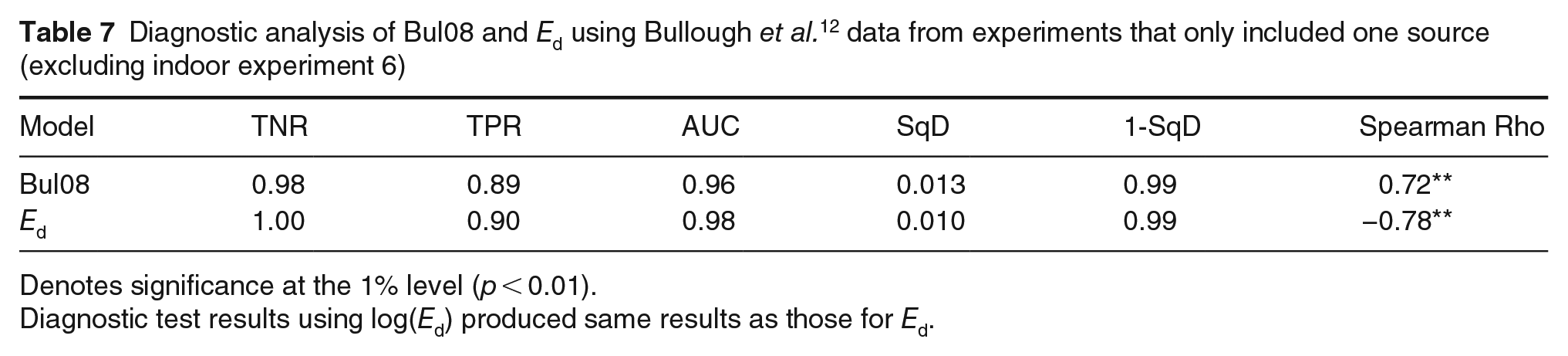
Denotes significance at the 1% level (p < 0.01).

Diagnostic test results using log(E_d) produced same results as those for E_d.

4.4 Limitations

There are several limitations to consider when interpreting the analyses presented in this article. Specifically, they are applicable under the range of lighting conditions in the considered datasets (see Table 4).

In the four datasets considered in this article, E_d was measured facing (i.e. normal) to the light source (S13 and T18 datasets), and with the source off axis (V17 and T15 datasets). Future studies are recommended to compare these two illuminance measurement approaches.

For the comparison between E_d and Bul08, accounting for indirect and ambient illuminance might become crucial when comparing environments with a higher variation in indirect or ambient illuminance such as a busy city centre compared to a rural area. It is currently unclear how limited E_i and E_a ranges need to be in order to safely ignore them and only use E_d. To address this issue, it might be possible to develop different E_d thresholds that pertain to outdoor environments with different common E_i and E_a. Future studies are warranted to explore this further.

As mentioned in the introduction, a previous study found differences in glare ratings when participants viewed three different sources that provided the same illuminance at the eye.^14,15 However, the performance of Bul11, which includes a term for maximum luminance, was not reported,^14,15 and it has not been clearly evaluated in subsequent studies. Villa et al. calculated Bul11 using average luminance of the fixture instead of maximum luminance,²⁰ and Tyukhova and Waters reported correlations between ratings and combined predictions from Bul08 and Bul11.²⁴ Further studies are needed to compare the performance of Bul11 (which uses a maximum luminance term) to Bul08. Furthermore, surveys of the level of optical diffusion used in street lighting fixtures would help determine the practical importance of accounting for maximum luminance and source luminance uniformity in DG models.

There are only a few studies of discomfort from glare in the pedestrian context. The number of studies available for subsequent analysis is further reduced due to inconsistency between studies in measured and reported quantities. The four combined datasets present a wider range of lighting conditions for pedestrian applications than any one individual study. Including additional datasets with larger variations in source sizes, eccentricity, indirect illuminance, ambient illuminance, and/or background luminance may change the conclusions drawn.

The analysis did not consider dynamic viewing or multiple glare sources because it is currently unclear how these two conditions can be accounted for using the evaluated seven models. For Lin14, Lin15 and Sch74, Villa et al. found a similar performance for these models with one or two glare sources.²⁰ They also found that ratings made using a dynamic viewing procedure were generally lower than ratings made with a static viewing procedure. A multi-dataset evaluation of the models using more than one glare source and using a dynamic viewing procedure is warranted.

In the presented analyses, it was assumed in this study that the comfort/ discomfort threshold in the 9-point scale was drawn just below 5. Further work is needed determine whether the conclusions are robust to changes in this assumption.

In two of the datasets, the sample sizes were quite small. While the sample sizes for V17 and T18 exceeded 30, those for the individual experiments within S13 and T15 ranged from 6 to 19. Small sample sizes can reduce a study’s power and ability to detect certain effect sizes.^42,43

Further studies are needed to verify the presented results and evaluate other models, such as Bul11, the European model (R_GI),⁴⁴ modified Daylight Glare Index (DGI),²¹ and the CIE maximum luminous intensity; the threshold is recommended by CIE for controlling glare in pedestrian situations.⁴⁵ These models were omitted from the current analysis because L_max, which is needed to calculate Bul11 (see Equation 5), and maximum luminous intensity data were not available in all four datasets. The modified DGI was not included in the current analysis because it requires luminance distribution data which were not available. Lastly, luminous intensity and the projected luminous area are needed to calculate R_GI, which were also not available. Future analysis of these models can be made possible if studies were to consistently report all needed quantities as proposed in a recent article.⁴⁶

Finally, the four datasets used sources with different CCTs (4000 K, 5700 K and 6500 K for V17, T18 and S13, respectively: T15 reported a CCT of 5000 K for only their first experiment). While there is some evidence that variations in glare source spectral power distribution affect discomfort evaluations this was not evaluated in the current analysis.^29,47,48

5. Conclusion

In this paper, we explored the predictions of discomfort from glare in the context of pedestrian lighting given by seven models tested using four independent datasets. For the range of experimental conditions used in these four datasets, we conclude that direct illuminance E_d is the most suitable model, as it tended to offer similar or better predictions than did the other models. The mean performance of E_d is slightly lower than Bul08, the model proposed by Bullough et al.¹² which exhibited the best performance, but Bul08 requires additional measurements that may not be straightforward to predict at design stage or to measure in the field. While the mean performance of E_d is slightly lower than Bul08, it offers a simpler approach for design and installation practice. For situations that deviate from the experimental conditions of the included datasets, the above conclusions should be considered tentative pending further research using more datasets and testing other metrics, such as Bul11.

Footnotes

Appendix A

Test results by dataset:

Appendix B

To evaluate whether one study influenced the findings more than others (using the combined data set), we conducted additional analyses similar to those shown in Table 5 but each time removing a different study dataset from the combined dataset. The Table B1 shows the mean performance for each model under each dataset removal scenario.

Similar to the reported results using all four datasets, we found that Bul08 had the highest mean performance in all scenarios. In the scenarios with T18 or S13 removed, Ed and Lin15 followed as having the second highest mean performance. In the scenario with V17 removed, E_d had the same mean performance as Bul08 whereas Lin15 had a slightly lower mean performance than Lin14. In the scenario with T15 removed, Sch74 had the same mean performance as Lin15, followed by E_d and L_avg. Although there were ties introduced when T15 was removed, the additional analyses showed that the reported findings using the combined dataset with four datasets still hold.

Acknowledgements

We would like to thank the authors of the four studies for sharing their experimental data and answering our questions. We would also like to thank Kate Hickcox for reviewing an initial draft of the article.

Declaration of conflicting interests

The authors declared no potential conflicts of interest with respect to the research, authorship, and/or publication of this article.

Funding

The authors disclosed receipt of the following financial support for the research, authorship, and/or publication of this article: This work was supported by the U.S. Department of Energy’s Lighting R&D Program, part of the Building Technologies Office within the Office of Energy Efficiency and Renewable Energy (EERE).

ORCID iDs

B Abboushi

S Fotios

N Miller

References

Commission Internationale de l’Éclairage. Disability glare, discomfort glare. ILV: International Lighting Vocabulary. CIE S 017/E:2020, 2nd edition. Vienna. https://cie.co.at/e-ilv (2020).

Illuminating Engineering Society. Lighting Science: Nomenclature and Definitions for Illuminating Engineering. ANSI/IES LS-1-22. New York: IES, 2022.

Ashdown

. Sensitivity analysis of glare rating metrics. Leukos 2005; 2(2): 115–122.

Commission Internationale de l’Éclairage. Discomfort glare in interior lighting. CIE 117:1995. Vienna: CIE, 1995.

Commission Internationale de l’Éclairage. Discomfort glare in road lighting and vehicle lighting. CIE 243:2021. Vienna: CIE, 2021.

Commission Internationale de l’Éclairage. Glare and uniformity in road lighting installations. CIE 031-1976. Vienna: CIE, 1976.

Vos

. Reflections on glare. Lighting Research and Technology 2003; 35: 163–176.

Lehnert

. Disability and discomfort glare under dynamic conditions – the effect of glare stimuli on the human Vision. In: Progress in automodile lighting (ed Schmidt-Clausen

H-J

), Munchen, 25–26 September 2001: 582–592.

Petherbridge

Hopkinson

. Discomfort glare and the lighting of buildings. Transactions of the Illuminating Engineering Society 1950; 15: 39–79.

10.

Lin

Liu

Sun

Zhu

Lai

Heynderickx

. Model predicting discomfort glare caused by LED road lights. Optics Express 2014; 22: 18056.

11.

Schmidt-Clausen

H-J

Bindels

JTH

. Assessment of discomfort glare in motor vehicle lighting. Lighting Research and Technology 1974; 6: 79–88.

12.

Bullough

Brons

Rea

. Predicting discomfort glare from outdoor lighting installations. Lighting Research and Technology 2008; 40: 225–242.

13.

Lin

Fotios

Wei

Liu

Guo

Sun

. Eye movement and pupil size constriction under discomfort glare. Investigative Ophthalmology and Visual Science 2015; 56: 1649–1656.

14.

Bullough

Hickcox

Narendran

. A method for estimating discomfort glare from exterior lighting systems. Lighting Research Center, Troy, NY.

15.

Bullough

. Luminance versus luminous intensity as a metric for discomfort glare. In: SAE 2011 World Congress & Exhibition, Detriot, MI, 12–14 April 2011, paper no. 2011-01-0111.

16.

City of Seattle. Street And Pedestrian Lighting, Retrieved on 25 September 2022 from https://streetsillustrated.seattle.gov/design-standards/lighting/.

17.

Colorado Department of Transportation. Lighting Design Guidelines for the Colorado Department of Transportation. Denver, CO: CDOT, 2020.

18.

Fotios

Uttley

Cheal

Hara

. Using eye-tracking to identify pedestrians’ critical visual tasks, Part 1. Dual task approach. Lighting Research and Technology 2015; 47: 133–148.

19.

Foulsham

Walker

Kingstone

. The where, what and when of gaze allocation in the lab and the natural environment. Vision Research 2011; 51: 1920–1931.

20.

Villa

Bremond

Saint-Jacques

. Assessment of pedestrian discomfort glare from urban LED lighting. Lighting Research and Technology 2017; 49: 147–172.

21.

Kohko

Ayama

Iwata

Kyoto

Toyota

. Study on evaluation of LED lighting glare in pedestrian zones. Journal of Light and Visual Environment 2015; 39: 15–25.

22.

Sivak

Flannagan

Traube

Kojima

. The influence of stimulus duration on discomfort glare for persons with and without visual correction. Transportation Human Factors 1999; 1: 147–158.

23.

Cohen

. Statistical Power Analysis for the Behavioural Sciences. 2nd ed. Mahwah: Lawrence Erlbaum Associates, 1988.

24.

Tyukhova

Waters

. Discomfort glare from small, high-luminance light sources when viewed against a dark surround. Leukos 2018; 14: 215–230.

25.

Wienold

Iwata

Sarey Khanie

Erell

Kaftan

Rodriguez

, et al. Cross-validation and robustness of daylight glare metrics. Lighting Research and Technology 2019; 51: 983–1013.

26.

Girard

Villa

Brémond

. Discomfort glare from several sources: a formula for outdoor lighting. Leukos 2021; 17: 108–124.

27.

Bullough

Van Derlofske

. Discomfort and disability glare from halogen and hid headlamp systems. In: SAE 2002 World Congress. Detroit, MI, 4–7 March 2002, paper no. 2002-01-0010.

28.

Bullough

Sweater Hickcox

. Interactions among light source luminance, illuminance and size on discomfort glare. SAE International Journal of Passenger Cars – Mechanical Systems 2012; 5: 199–202.

29.

Sweater-Hickcox

Narendran

Bullough

, et al. Effect of different coloured luminous surrounds on LED discomfort glare perception. Lighting Research and Technology 2013; 45: 464–475.

30.

Tashiro

Kawanobe

Kimura-Minoda

Kohko

Ishikawa

Ayama

. Discomfort glare for white LED light sources with different spatial arrangements. Lighting Research and Technology 2015; 47: 316–337.

31.

Tyukhova

. Discomfort glare from small, high luminance light sources in outdoor nighttime environments. PhD Thesis, University of Nebraska – Lincoln, USA. 2015.

32.

de Boer

Schreuder

. Glare as a criterion for quality in street lighting. Transactions of the Illuminating Engineering Society 1967; 32: 117–135.

33.

Quincey

. The range of options for handling plane angle and solid angle within a system of units. Metrologia 2016; 53: 840–845.

34.

Sheskin

. Handbook of Parametric and Nonparametric Statistical Procedures. Boca Raton: CRC Press, 1997.

35.

Holm

. A simple sequentially rejective multiple test procedure. Scandinavian Journal of Statistics 1979; 6: 65–70.

36.

Safari

Baratloo

Elfil

Negida

. Evidence Based Emergency Medicine; Part 5 Receiver Operating Curve and Area under the Curve. Emergency (Tehran, Iran) 2016; 4: 111–113.

37.

Rodriguez

Yamín Garretón

Pattini

. An epidemiological approach to daylight discomfort glare. Building and Environment 2017; 113: 39–48.

38.

Akobeng

. Understanding diagnostic tests 3: Receiver operating characteristic curves. Acta Paediatrica 2007; 96: 644–647.

39.

Marchant

. Do brighter, whiter street lights improve road safety? Significance 2019; 16: 8–9.

40.

Hussain

. Comparison of real-world roadway lighting, dynamic simulation and CBE and Glare mark predictive systems. Master’s thesis. Manhattan, KS: Kansas State University, KS, 1985.

41.

Sing

Sander

Beerenwinkel

Lengauer

Unterthiner

Ernst

. The ROCR Package. R vignette, https://cran.rstudio.com/web/packages/ROCR/vignettes/ROCR.html (2020).

42.

Bujang

Adnan

. Requirements for Minimum Sample Size for Sensitivity and Specificity Analysis. Journal of Clinical and Diagnostic Research JCDR 2016; 10: YE01–YE06.

43.

Uttley

. Power analysis, sample size, and assessment of statistical assumptions—improving the evidential value of lighting research. Leukos 2019; 15: 143–162.

44.

European Committee for Standardisation Road Lighting – Part 2: Performance Requirements. CEN 13201-2:2015. Brussels: CEN, 2015.

45.

Commission Internationale de l’Éclairage. Lighting of roads for motor and pedestrian traffic. CIE 115:2010. Vienna: CIE, 2010.

46.

Abboushi

Miller

. What to measure and report in studies of discomfort from glare for pedestrian applications. Lighting Research and Technology. First published 24 June 2022; DOI: 14771535221087133.

47.

Yang

Luo

Huang

. Assessing glare, Part 3: Glare sources having different colours. Lighting Research and Technology 2018; 50: 596–615.

48.

Pierson

Wienold

Bodart

. Review of factors influencing discomfort glare perception from daylight. Leukos 2018; 14: 111–148.

Predicting discomfort from glare with pedestrian-scale lighting: A comparison of candidate models using four independent datasets

Abstract

1. Introduction

2. Method

2.1 Evaluated models

2.2 Study and data inclusion criteria

2.3 Included studies and datasets

2.4 Model performance evaluation

2.5 Assumptions

3. Results

4. Discussion

4.1 Combined dataset

4.2 Individual datasets

4.3 The performance of Ed using Bul08 model development data

4.4 Limitations

5. Conclusion

Footnotes

Appendix A

Appendix B

Acknowledgements

Declaration of conflicting interests

Funding

ORCID iDs

References

4.3 The performance of E_d using Bul08 model development data