
Abstract
Multi-primary tunable LED lighting systems can generate a vast number of spectral outputs, with the exact number depending on the resolution of the control signal and number of LED primaries. Computing all combinations to identify optimal spectral power distributions (SPDs) with a specified chromaticity would require a tremendous amount of time and computational power. Here, an enumeration reduction (ER) algorithm is described to reduce the computation time by defining a bounding pyramid in the three-dimensional tristimulus space that maps to the circumscribed square of the target region in the chromaticity diagram. This method enables computing only the necessary amount of tristimulus values (and resulting chromaticity coordinates) for SPDs that fall into a user-defined target chromaticity area, reducing computation time by avoiding the need to generate each combination and calculate its chromaticity coordinates. The results show that the proposed ER algorithm can greatly reduce the time – up to 922 times in a series of tests – to determine a set of metamers compared to a full enumeration computation.
1. Introduction
1.1 Multi-primary lighting systems
Solid-state lighting (SSL) devices have become increasingly prevalent due to their efficiency, compact size, robustness, lifetime, spatial and spectral output control, and ability to be dimmed. SSL devices, such as LEDs, utilize additive colour mixing principles to generate white light, with energy radiated directly from the diode or from phosphors that down convert energy in shorter wavelengths to energy in longer wavelengths (i.e. Stoke’s shift). The most common type of LED system in use today relies on a nominally blue ‘pump’ LED and phosphors that produce nominally green, yellow, orange and red light, which in combination produces white light. These products provide a single, fixed output at full power, such that system performance is straightforward to measure and report. They are cost-effective and can have the highest efficacy of any available light source.
White light can also be generated by mixing the output of multiple LEDs, such as nominally red-, green- and blue-emitting diodes, with each referred to as a primary. Because the output of each primary can be controlled independently, multi-primary LED (mpLED) systems can offer flexibility in spectral output, with a single product capable of delivering a wide range of spectral power distributions (SPDs). This can allow the performance of a lighting system to vary after installation, being optimized over the course of use for colour quality, 1 non-visual stimulation, 2 consistency of appearance, 3 energy efficiency, 4 daylight and electric lighting balance, 5 horticultural effectiveness 6 or other attributes. MpLED systems are also of interest because they offer a higher theoretical maximum luminous efficacy due to their potential elimination of Stoke’s shift losses and ability to deliver a more tailored SPD comprised of specific narrowband components. The U.S. Department of Energy projects mpLED systems to be the most efficacious light source by the 2030s. 7
In different lighting applications, optimization targets (i.e. photometric, colorimetric and circadian metrics) can vary, and finding the optimal combinations of spectral primaries to meet any given parameter might require an extensive search, resulting in a long processing time. For example, determining the SPDs with chromaticity of 3500 K (threshold radius rt = 0.0005) among combinations produced from 16 LED primaries at just 20% output increments (0%, 20%, 40%, 60%, 80% and 100%) took 96 core hours (1 wall clock hour on four 24 core nodes) at the Pacific Northwest National Laboratory’s (PNNL) Computational Science Facility in Richland, Washington – PNNL’s Constance cluster is composed of 528 nodes each with 24 core Intel® Haswell E5-2670 v3 (running at 2.3 GHz) with 64 GB of 2133 MHz ECC memory and connected through fourteen data rate InfiniBand™ network card. For nominal white light combinations that fell within an area close to Planckian radiation defined by ANSI, 8 colour rendering metrics, such as ANSI/IES TM-30 fidelity index Rf, gamut index Rg and local chroma shifts Rcs,hi were calculated. Despite the long calculation time, this result is still too coarse for practical use.
The number of possible spectral output states of an mpLED system is equal to the number of control increments raised to the number of primaries. For example, a system with 8-bit control (256 levels) and 5 primaries can generate 256 5 (1,099,511,627,776) unique conditions. To reduce the computational burden, the search space – defined as all the possible spectral power combinations in an mpLED system – could be limited to a particular region of chromaticity, perhaps even one small enough to contain only visually indistinguishable lights. However, there is currently no method for searching only this limited range, and instead the chromaticity of all combinations must be computed and checked against a criterion. Addressing this problem by utilizing the tristimulus values (TSVs) of the primaries is shown in this work to provide substantial computational time savings. The proposed enumeration reduction (ER) algorithm can help facilitate real-time computations and expedite computing and characterizing the performance of mpLED systems.
While only three primaries are necessary to produce mixtures of light with any chromaticity within their gamut, such systems cannot produce metamers, which are traditionally defined as two or more conditions having the same chromaticity but different SPDs. Metamers are important because they allow other performance attributes to vary while chromaticity is held constant, providing a useful tool for lighting practitioners to optimize performance without visible differences in the emitted light. Besides not delivering metamers, typical three-component mpLED systems do not offer adequate colour rendition for many architectural lighting applications.9–12 Given the limitations of three primary systems, four and five primary mpLED systems are the most common commercial products today. Nevertheless, products with up to eight primaries are readily available, and lighting systems intended for research may have more than 30 unique primaries. LED systems with several primaries can generate a vast number of combinations that have identical chromaticity, but varying SPDs, hence varying colour and melanopic qualities, as shown in Figure 1.
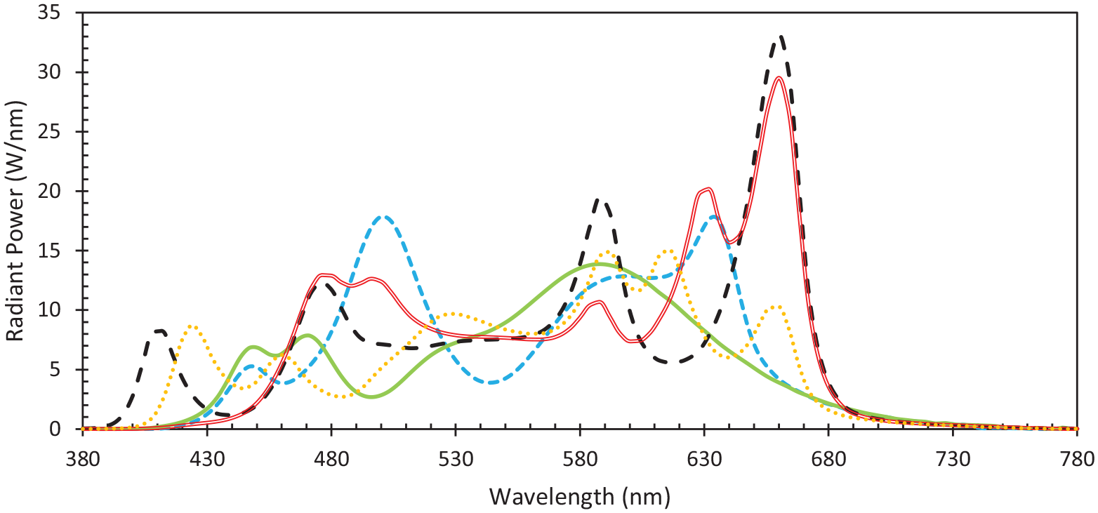
Demonstration of different spectral power distributions of lights, each represented by a different line type, having identical chromaticity (3500 K on the Planckian locus) that could be generated by a multi-primary LED system
Even with only four primaries, physical measurement of all combinations is not practical. However, estimation of combinations is possible by measuring the output of each primary. Once each primary is characterized, combinations can be determined mathematically to estimate the true performance of the physical combinations. In some cases, one measurement of each primary can be scaled to predict its output at any given output-control (i.e. power or drive current) level, although non-linear relationships between drive current and output characteristics are common. More measurements can allow for interpolation to predict the output of a primary at any given control state (i.e. a coefficient xi in the problem statement shown in Section 2 can be adjusted to accurately estimate the actual light output from each individual primary). This consideration is not within the scope of this article, which instead focuses on the enumeration aspect, rather than understanding the accuracy of estimations.
The evaluation of mpLED product performance is crucial in terms of market acceptance, usability and quality determination. A reliable and repeatable quantification of mpLED spectrum-based performance (e.g. colour rendition, melanopic stimulation) will enable manufacturers to build better performing products by optimizing the quantity and type of included primaries. There are two existing challenges: (1) determining ways to summarize performance that are useful and (2) efficiently computing the performance of estimated combinations. This article is focused on the latter, but with consideration for preliminary ideas for addressing the former.
1.2 Methods for quantifying estimated mpLED system performance
There are broadly two approaches to understanding the performance of estimated combinations. One is to perform single or multi-objective heuristic optimizations with specified performance criteria. This method produces a single result for each optimization that is used for addressing a specific goal, such as determining an experimental stimulus or, if multiple optimizations are completed, finding the Pareto boundary of two metrics. Computing optimal solutions is relatively fast – although not presently fast enough for real-time control – but requires some skill to program. This approach has been taken in numerous studies of LED system performance, with techniques including linear, 9 non-linear, 12 stochastic, 10 genetic, 11 multi-objective genetic, 13 swarm 14 and Nelder–Mead simplex 15 algorithms.
Alternatively, brute-force enumeration techniques can be utilized to generate large numbers of SPDs. This approach determines specified performance characteristics for all (or many) combinations that can be created from an mpLED system. This approach gives a broader characterization of the trade-offs between different performance attributes, and through a lookup table has the potential to facilitate real-time performance tuning. Enumeration enables one to identify patterns, detect anomalies and perform statistically sound analysis, 16 and is most useful when the specific aim of optimization is initially unknown or may vary. Carefully considered enumeration techniques can be preferable for understanding and reporting the performance of mpLED systems but can require substantial computation time and data storage. One recent work utilized a combination of heuristic optimizations and enumeration. 17
One initial step to reduce computational burden of enumeration is to characterize system performance with a discrete set of metamers, rather than across the full range of chromaticity – the range of chromaticity can be easily determined and reported separately. This is the starting point of this work. Because the practical output of each primary occurs at discrete levels, this requires consideration of the precision of metamer determination. That is, with discrete control levels, only a small number of true metamers exist, but by defining a small tolerance – taking the form of a radius – for the chromaticity of the metamers (rt), a much larger set of practical metamers can be created that are still visually equivalent in terms of the chromaticity of the light to a human observer. This region is deemed a target chromaticity area (TCA).
This article proposes a novel method for determining the combinations of primaries that are nominally metamers (i.e. have chromaticity within the TCA). The goal was to eliminate the need to determine the chromaticity of all possible combinations to check whether it falls within the TCA, and thus reduce the computational burden. To our knowledge, there is no alternative algorithm that serves this function; only objective-based optimizations and brute-force enumeration have previously been documented. After describing the proposed method, the article provides example results to demonstrate how it reduces the computation burden.
2. Proposed method
In an mpLED lighting system with n number of primaries, TSVs X, Y and Z are generated by scaling each primary using a coefficient (xi), as shown in Equations (1)–(3):


The TSVs are later converted to chromaticity scales and colour spaces. Solving this problem with a brute-force approach requires testing all combinations possible for the coefficients. For example, in a lighting system with 8-bit dimming control, each individual primary can be dimmed between 0 and 255 (xi = 0, 1, 2, . . ., 255).
At its core, the proposed ER algorithm is a way to predict metamers with calculations that are less burdensome than computing the chromaticity coordinates of every possible combination of primaries comprising a composite SPD. This is possible given the geometric relationship between TSVs and chromaticity coordinates. Chromaticity coordinates provide quantification of a colour stimulus generated by a light source in a two-dimensional diagram. The International Commission on Illumination (CIE) defines the CIE 1976
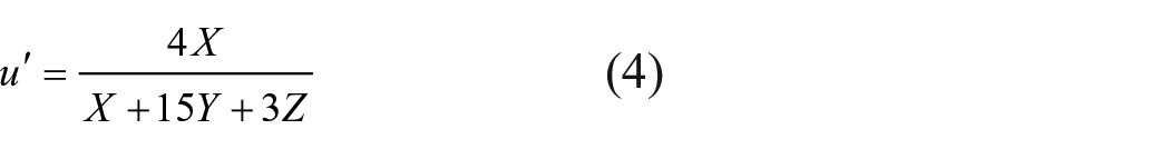
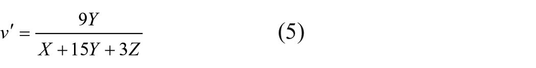
where X, Y and Z are TSVs, which are derived from the sensitivity of the human visual system. For more information, see CIE 15:2018. 18
The proposed algorithm avoids determining the chromaticity coordinates for every possible spectral output by first partitioning the TSVs of each individual LED primary into three groups based on the dominant coordinate
The definition of the limiting pyramid and directional distances is provided in the following sections. First, a simpler notion of a limiting quadrilateral will be presented in two dimensions in the
2.1 Geometric analysis of the chromaticity diagram
2.1.1 The limiting quadrilateral
The desired


where
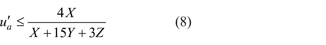
and since the TSVs X, Y and Z are all positive, this can become Equation (9):

Subtracting
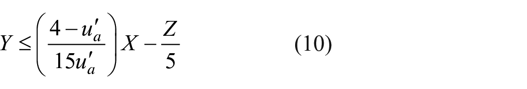
Similarly, Equation (11) can be derived from the
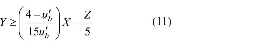
and the inequalities for bounds on v′ provides the following two relationships, provided in Equations (12) and (13):
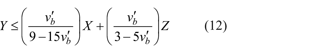
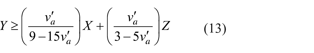
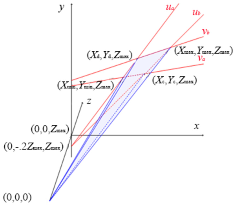
The inequalities in Equations (12) and (13) are elucidated in the X-Y plane for some fixed value of Z. For a fixed value of Z, the lines in the X-Y plane can be defined using Equations (10) through (13) where the limiting lines can be referred to as
Thus, for a fixed value of Z, values of X and Y that will result in chromaticity within the TCA must lie below the

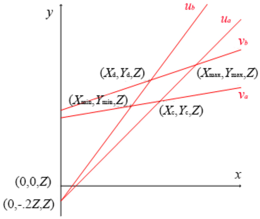
The limiting quadrilateral showing the boundaries of the tristimulus combinations selected for further analysis
where
For line

where
For line
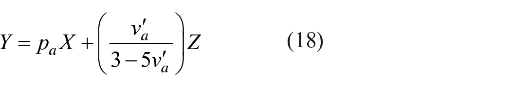
where
For line
where
The coordinates of the extreme corners of the limiting quadrilateral are

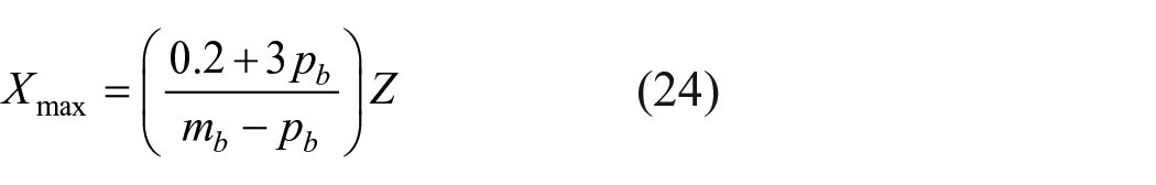

Once the Z component of the tristimulus triple is fixed, there are fairly narrow restrictions on the X and Y components for the triple to map to the TCA. It is also apparent that for a given set of TSVs, there is a maximum amount of X and Y components available (with all primaries at maximum output). The combination of the formulae for Xmin and Ymin yields the limit for the maximum amount of Z component that can be balanced by the available X and Y components to position the combinations within the TCA. The sum of the TSV X components for the included primaries can be denoted by Xtot and the sum of the TSV Y components can be denoted by Ytot. Since Xmin ⩽ Xtot and Ymin ⩽ Ytot, the geometric boundaries of the quadrilateral can be described as shown in Equations (26) and (27)
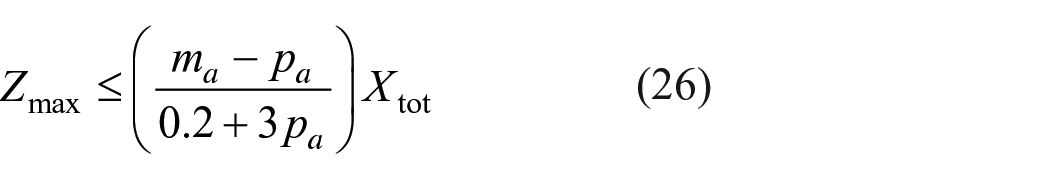
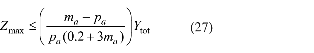
The smallest of these two bounds is Zmax.
2.1.2 The limiting pyramid
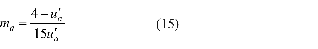
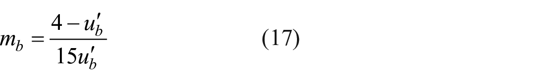
From the equations for the slopes of the
The limiting pyramid shows the three-dimensional boundary for the tristimulus values of the combined spectral power distributions
2.2 Directional distance
Directional distance between a point and a line or a plane is simply the Euclidian distance between them with a sign attached indicating on which side of the line or plane the point lies. This notion is first illustrated with an example in two dimensions and extended to three dimensions in Section 2.2.2.
2.2.1 Directional distance in two dimensions
Figure 4 shows a graph of the line

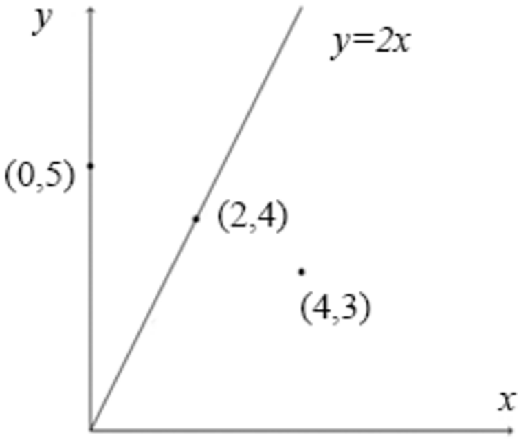
Directional distance, the distance between a point and y = 2x line, is used to sort out the outcomes on the limiting quadrilateral
This line can be denoted as
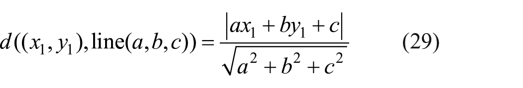
A normalized standard form of the line is shown in Equation (30):

The directional distance, which is denoted

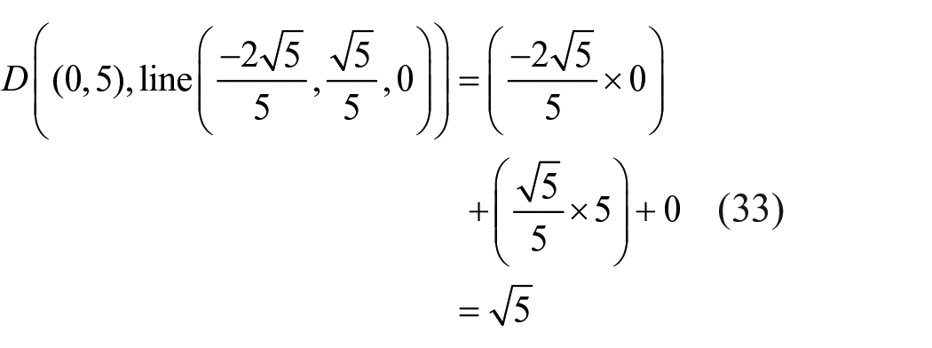
In Figure 3, the normalized standard form of

The directional distance from point (0,5) to
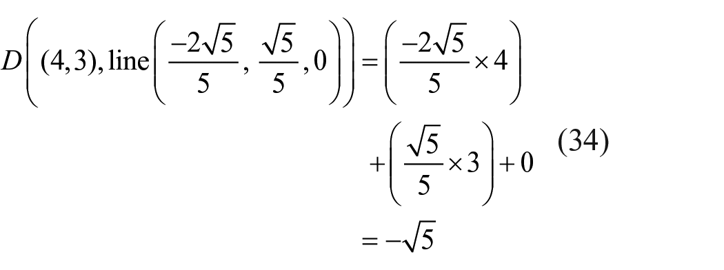
The directional distance from point (4,3) to
2.2.2 Directional distance in three dimensions
Directional distance in three dimensions is directly analogous to the two-dimensional definition. The standard form for the equation of a plane in variables

A particular plane specified in Equation (32) can be denoted as

The planes of interest in the enumeration process will be the planes swept out by the
2.2.3 Additive property of directional distances
An important property of directional distances that they are additive. When forming combinations of two TSVs, the directional distance of their sum from a given plane is the sum of their directional distances from that plane. Equation (37) follows directly from Equation (36):

2.3 ER algorithm
A rough outline of the process is given below (steps 1–9), and subsequent subsections will elaborate on the individual steps.
Determine the normalized coefficients of the vb plane and ub plane.
Sort the primaries into three groups based on the dominant coordinate of their TSV (Xp1, Yp1, Zp1), (Xp2, Yp2, Zp2), . . ., (Xpn, Ypn, Zpn) for n number of primaries.
Within each group, form all possible output and primary SPD combinations (Xx,com, Yx,comp, Zx,com), (Xy,com, Yy,com, Zy,com), (Xz,com, Yz,com, Zz,com).
Sort the Z-dominant combinations by their TSV Z component (Xz,com, Yz,com, Zz,com) and store the sorted list of TSV combinations in a file removing those combinations with Z component greater than
Sort the Y-dominant combinations by their directional distance from the vb plane (Xy,com, Yy,com, Zy,com) and store the sorted list of TSVs. Also bin the sorted list into a number of fixed width bins, determining the index in the sorted list of the first element in each bin. These bin indices, the bin width, the minimum and maximum directional distance from the vb plane, and the minimum and maximum directional distance from the ub plane are stored.
Similarly sort the X-dominant combinations by their directional distance from the ub plane (Xx,com, Yx,com, Zx,com), storing the sorted list along with the two directional distances for each combination and the minimum and maximum directional distances from each of the two limiting planes. Also bin this sorted list into fixed width bins, storing the bin width and bin indices in the sorted list.
For each Z-dominant combination, compute its directional distance from the
For each Z-dominant plus Y-dominant combination, denoted as a
For each of these
2.3.1 The
and
plane equations
The equations of the
The points for the
The points used to determine the equation of the
2.3.2 The coordinate-dominant regions of TSV space
All possible combinations of a set of TSVs at all discrete output-control levels lie in a box with lower left corner at the origin (all output levels are zero) and upper right corner
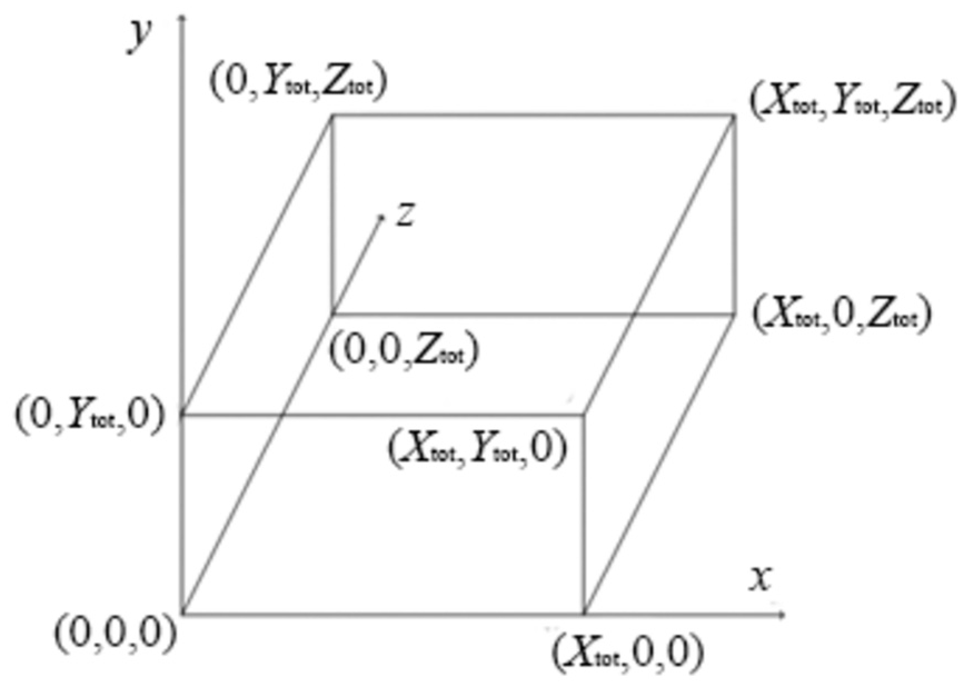
All tristimulus value combinations range showing the boundaries of Xtot, Ytot and Ztot in a box
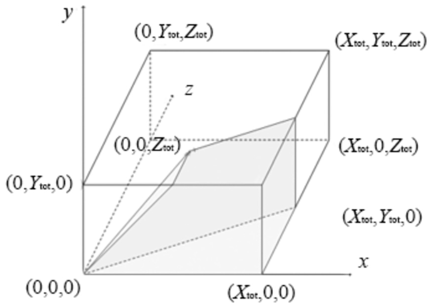
X-dominant tristimulus value combinations range
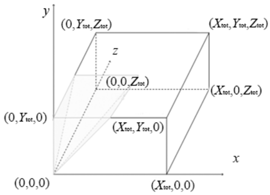
Y-dominant tristimulus value combinations range
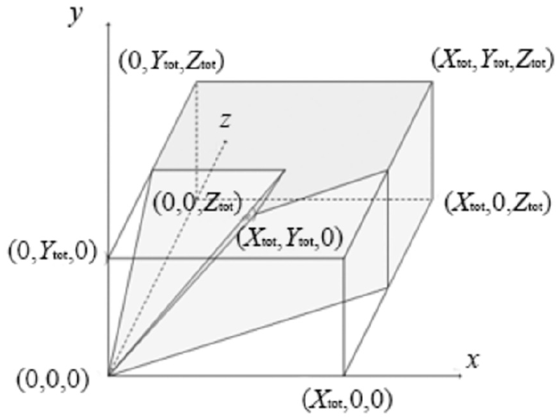
Z-dominant tristimulus value combinations range
2.3.3 The sorted Z-dominant TSVs
For combinations of the Z-dominant TSVs, three coordinates in three eight-byte binary floating-point numbers (doubles) are stored, as the directional distances are computed just once in step 7 of the ER method. Any combination that has a
2.3.3 The sorted Y-dominant TSVs
The Y-dominant TSVs and their directional distances from the
If there are
2.3.4 The sorted X-dominant TSVs
The X-dominant TSVs and their directional distances from the
If there are
2.3.5 Combining dominant-coordinate group combinations that could land in the TCA
In steps 7–9 of the of the ER algorithm forming all the
If the maximum distance between the

Similarly, the maximum distance between the

Thus, a tristimulus combination that maps to the TCA must have its directional distance from the

The

As the Y-dominant TSVs are sorted by their directional distance from the
where
The last bin index,
In a similar fashion, for a given Z-dominant TSV combination paired with each Y-dominant TSV combination in bins

Analogously, and with the definitions in Section 2.3.5, it is evident that the delimiting indices for the X-dominant TSV combinations bins,
2.3.6 Parallel implementation of the ER algorithm
Steps 1 through 6 in the ER algorithm take very little time and are run serially in a program called gen_combos to generate the sorted coordinate-dominant TSV groups with their corresponding directional distances from the
3 Performance evaluation
A test was performed to capture the benefits of the ER algorithm by comparing the calculation time needed to generate a metamer set for the proposed method to that of a full enumeration. In all, 12 theoretical mpLED systems were established by calculating primaries as Gaussian distributions. The 12 mpLED systems included three systems with four primaries, three systems with five primaries, three systems with six primaries and three systems with seven primaries. The data comprising these systems are available as supplemental material. A TCA was centred on the Planckian locus with a colour temperature of 3500 K, chromaticity coordinates
For each mpLED system, a full enumeration was calculated using the Constance computer previously described, with the chromaticity of each spectral combination of LED primaries checked for compliance with the TCA criterion of 3500 K on Planckian locus with a
Results of wall clock time comparisons for the ER algorithm and full calculation of all combinations
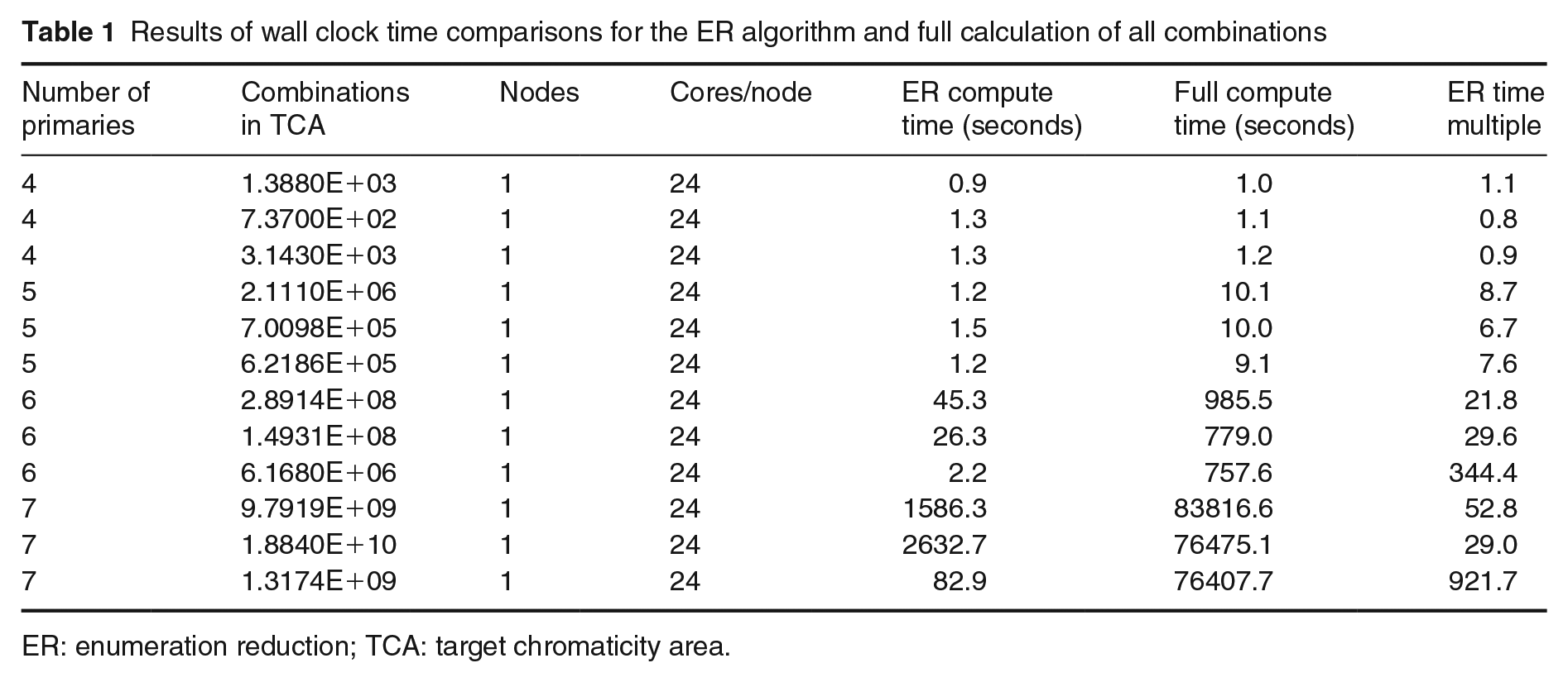
ER: enumeration reduction; TCA: target chromaticity area.
As shown in Table 1, the ER algorithm reduced the time to find the set of metamers (i.e. combinations with a chromaticity within the TCA) by up to 99.89%. However, the reduction in time was highly variable, depending on both the number of primaries and the number of combinations within the TCA. The number of combinations in the TCA computed on one core, not provided, is also a factor. Likewise, the full computation varies slightly for systems with the same number of primaries due to differences in parallel computing.
For four primary systems, the ER algorithm offered no benefit because the time needed to determine and sort the groups of TSVs offset any reduction in chromaticity coordinate calculations. Likewise, there were only modest benefits for five primary systems. As the number of primaries increased, the benefit of the ER algorithm also increased, and the algorithm is anticipated to be essential for understanding the performance of research-grade mpLED systems with eight or more primaries. Table 1 is limited to a maximum of seven primaries because the cost and calculation time associated with a full enumeration of combinations for eight primary systems became unjustifiable. Running on 30 nodes, the ER algorithm for three computed eight primary mpLED systems took between 130 and 12,026 seconds. The calculation time for the baseline full enumeration of an eight primary mpLED systems could be expected to take days, even on a high-performance computer.
The ER algorithm showed more benefit for mpLED systems with fewer combinations falling within the TCA for a given number of primaries because more chromaticity coordinate calculations could be avoided. It is important to remember that the ER algorithm does not result in chromaticity coordinates itself, but a set of combinations for which chromaticity is calculated. The set is slightly larger than what is in the TCA, so some combinations identified by the ER algorithm are ultimately not kept in the metamer set.
Two possible improvements to the ER algorithm are apparent with a possibility of additional overhead. The first is to sort the Z-dominant TSVs by their directional distance from the
4 Conclusions
While tunable, mpLED systems can emit a vast number of spectral outputs, calculating and describing these lighting conditions requires a tremendous amount of computational time and data storage. Among a broader set of methods being developed to improve the efficiency and impact of mpLED system assessments, a new method, denoted the ER algorithm, was developed to predict the combinations of LED primaries that will fall within a specified area of a chromaticity diagram. Using this method, chromaticity coordinates for only a small subset of the total spectral outputs that can be generated by a system need to be calculated to identify a set of nominal metamers (i.e. having chromaticity coordinates within the specified area). For a set of 12 theoretical mpLED systems, the ER algorithm reduced the time to determine a set of nominal metamers by up to 99.89%. More benefit was found for systems with more primaries, and with a lower percentage of all possible combinations having chromaticity coordinates within the area of interest, which varies based on the specific primaries included in the system. The ER algorithm offers substantial benefit for researchers trying to understand the performance of products and for engineers trying to quantify and market product performance.
Footnotes
Declaration of conflicting interests
The authors declared no potential conflicts of interest with respect to the research, authorship and/or publication of this article.
Funding
The authors disclosed receipt of the following financial support for the research, authorship and/or publication of this article: This work was supported by the U.S. Department of Energy’s Lighting R&D Program, part of the Building Technologies Office within the Office of Energy Efficiency and Renewable Energy (EERE).
Replication of results
Details of the optimization algorithm have been provided in this manuscript to enable others to replicate the results of the proposed method. Due to the large file size of the data collected using this algorithm, the raw calculation data have been omitted, except for one example made available via GitHub. Code for the ER algorithm is available from GitHub: ![]() . Example data are also provided.
. Example data are also provided.