The transition between lit and unlit sections of road and detection of driving hazards after dark

Abstract

An experiment to investigate peripheral detection performance during a driver’s transition between lit and unlit sections of road was undertaken. The results suggest that when a driver moves from a lit to an unlit section of road their detection performance decreases almost immediately to that expected for the conditions of the unlit section and that there is no significant change in the subsequent 20-minute period. Tests were conducted at three luminances (0.1, 1.0 and 2.0 cd/m²): while an increase from 0.1 to 1.0 cd/m² improved detection, a further increase to 2.0 cd/m² did not. Lighting of two S/P ratios (0.65, 1.40) was examined at 1.0 cd/m²: this did not suggest an effect on detection performance. Taken together, these results suggest that, in the current context, visual performance reached a plateau at 1.0 cd/m².

1. Introduction

The purpose of road lighting on main roads is to allow the drivers of motorised vehicles to proceed safely, specifically to provide visual cues and reveal potential hazards so that safe vehicular operation is possible. ¹ Road lighting reveals objects that are beyond the reach of vehicle forward lighting, which can potentially occur frequently at higher speeds. ²

Many aspects of visual performance deteriorate under reduced lighting conditions: spatial resolution, contrast discrimination, stereoscopic depth perception, accommodation response and reaction time. ³ An extreme case of ‘reduced lighting’ is the absence of road lighting. Not all sections of a main road are lit after dark. The decision to install lighting may consider the likely cost–benefit of lighting provision versus accident reduction. ⁴ Lighting is not an effective countermeasure for all types of road accident^5,6 and that may guide consideration of use. Furthermore, installed lighting may be switched off for some part of the after-dark period as an energy saving measure.

The transition from lit to unlit sections of road will affect a driver’s state of adaptation. For a lit section, road lighting on main roads is typically designed to provide surface luminances in the range of 0.3–2.0 cd/m². ¹ For an unlit section, this will be reduced according to the contributions of headlamps, moonlight and extraneous light sources. Visual adaptation is the process of adjusting to the quantity and quality of light and this process is mediated through changes in pupil size, neural adaptation and photochemical adaptation. ⁷ Luminance changes of 2–3 log units are likely to be handled by the neural system which responds relatively fast, typically less than 200 ms. ⁷ Adaptation to greater changes in luminance will involve changes in pupil size and photochemical adaptation, and hence the relative contributions in peripheral vision of the rod and cone receptors.

This paper describes an experiment carried out to investigate detection in peripheral vision across the transition between lit and unlit (and vice versa) sections of road. This was done using a scale model simulating the visual scene of a driver to determine how detection performance was affected by the sudden transition and subsequent long-term adaptation.

2. Apparatus

Hazard detection was investigated using a 1:10 scale model simulating a driver’s view of a road. The driver was located in the middle lane of a three-lane carriageway. The road was lit by the driver’s own head-lighting on a dipped setting (these were switched on for all trials) and by two arrays of LEDs simulating overhead road lighting. Two detection tasks were carried out in parallel – detection of a suddenly appearing obstacle in the road ahead and detection of one or other of the two vehicles ahead moving into the driver’s lane. A dynamic fixation task was used to add cognitive load during trials and to direct attention ahead rather than onto the detection tasks. The effect of the lit–unlit transition was analysed by comparing the frequency of correct detection responses and the reaction time of these responses. Reported here is a summary of the apparatus: a more complete description is reported elsewhere.^8,9

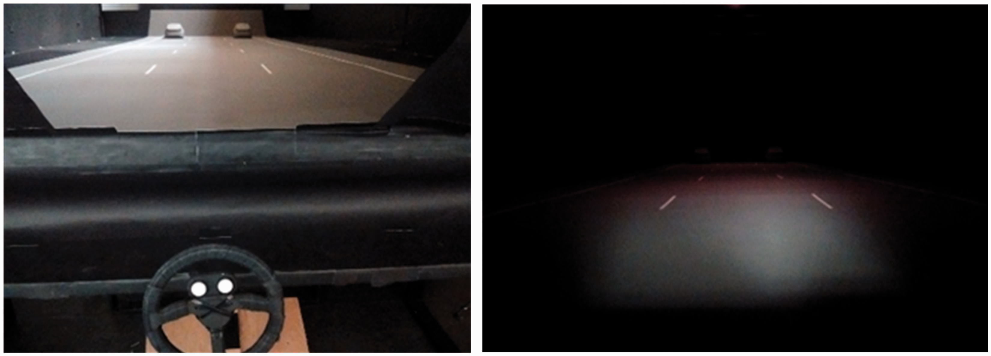
Figure 1 shows the test chamber, this having dimensions approximately 5 m long, 2.5 m wide and 1.5 m high. A driver–participant sitting outside the chamber viewed the interior through an acrylic windscreen (Figure 2), placing their horizontal sightline approximately 150 mm above the chamber floor (the road surface), with the top of the windscreen being 200 mm above this surface. When seated and looking towards the fixation mark, test participants were not able to see the LED arrays directly. The chamber floor was painted in neutral grey (Munsell N5) to represent an asphalt road surface and other interior surfaces were painted matt-black. The back wall of the chamber was a dark grey rear-projection screen.

Figure 1.

Plan and section of the test chamber showing the detection targets, overhead road lighting, vehicle forward lighting and viewing position.

Figure 2.

Left: The participant’s view of the road ahead, showing the detection-response buttons on the steering wheel. Right: the view ahead as lit only by the driver’s headlights. Note: laboratory lighting switched on for left-hand photograph to reveal the steering wheel: this lighting was switched off during all trials.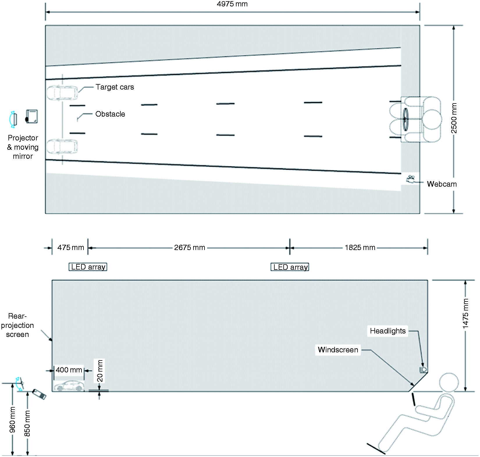

2.1. Lighting

Road lighting was simulated by two LED luminaires located above transparent sections of the ceiling (Figure 1). Table 1 shows the light settings used in this work. The luminances were chosen to represent those typical on UK roads ¹⁰ with the log unit difference employed with the expectation of revealing a significant effect on detection. Two spectra were chosen, these representing the scotopic/photopic (S/P) ratio of high pressure sodium (HPS, S/P = 0.65) and metal halide (MH, S/P = 1.40) lighting.

Table 1

Summary of lighting conditions

Light setting	Nominal luminance (cd/m2)	S/P ratio	Chromaticity (CIE 2 degree)
			x	y
1	1.0	0.65	0.54	0.41
2	0.1	1.40	0.46	0.41
3	1.0	1.40	0.46	0.41
4	2.0	1.40	0.46	0.41

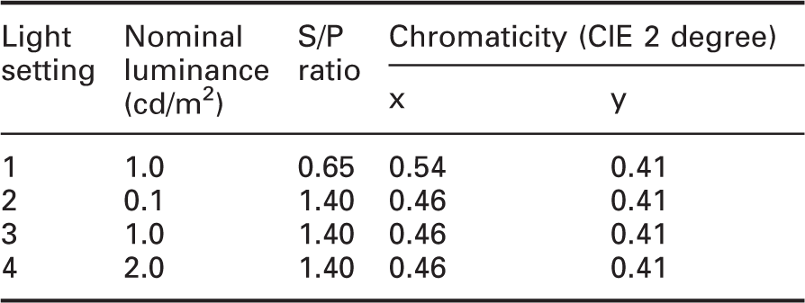
Road surface luminance was measured along the centreline of the middle lane, using a Konica-Minolta LS110 Meter with a ⅓° capture field, with the luminance meter in the location of the test participant as a driver (but without the windscreen). Measurements were recorded at 0.5 m intervals starting at 0.45 m from the far wall (i.e. directly underneath the further LED array). The nominal luminances shown in Table 1 are those at the location of the detection targets. Considering only those luminances measured between the two LED arrays (simulating road lighting at a spacing of 27 m), the mean luminance was 0.87 that of the nominal luminance and with a longitudinal uniformity (minimum/maximum) of 0.58. For the nominal luminance of 1.0 cd/m², the minimum and maximum luminances were 0.62 cd/m² and 1.08 cd/m², respectively.

Low beam forward lighting from the participant’s vehicle was simulated using two white LEDs (4000 K). The beam pattern was produced using individual LED lenses and fine-tuned with small adjustable barn doors and opaque masking tape. Beam intensity was controlled with a dimmable constant-current LED driver. The visual impact of the forward lighting is shown in Figure 2. Vertical illuminances from the headlights were 0.16 lux at the obstacle and 0.13 lux and 0.17 lux in front of the left-hand and right-hand cars, respectively. For this work, the headlamps were used to enhance the apparent simulation (i.e. to promote ecological validity) within a study of road lighting rather than to purposefully illuminate the detection objects, and thus these illuminances are lower than typical. ¹¹

2.2. Detection tasks

Test participants were required to detect two events; the appearance of a static obstacle on the road ahead and a car slightly ahead moving into the same lane. In the scale model, the driver was located in the middle lane of a three-lane carriageway. The obstacle was also located in the middle lane. The target cars were located in the nearside and offside lanes, with their movement into the middle lane being the detection event. All three targets were located 4.7 m ahead of the driver’s eyes and scaled to represent the visual sizes of real targets at 47 m.

The target cars were 1/10th scale models (Figure 3) painted the same neutral grey (Munsell N5) as the road surface. Tail lights were switched off during trials so that detection performance was a function only of changes in road lighting. To enable lane-changing movements, they were connected through a slot in the road surface to a linear guide rail. Lane change motion simulated the typical speed of a lane change ¹² with the lane-centre to lane-centre movement being completed in 6 seconds. Participants were instructed to press the steering wheel button when they detected the cars move from the home to the middle lane.

Figure 3.

Photograph (from the side, not from the driver’s viewpoint) of a target car and the raised road surface obstacle.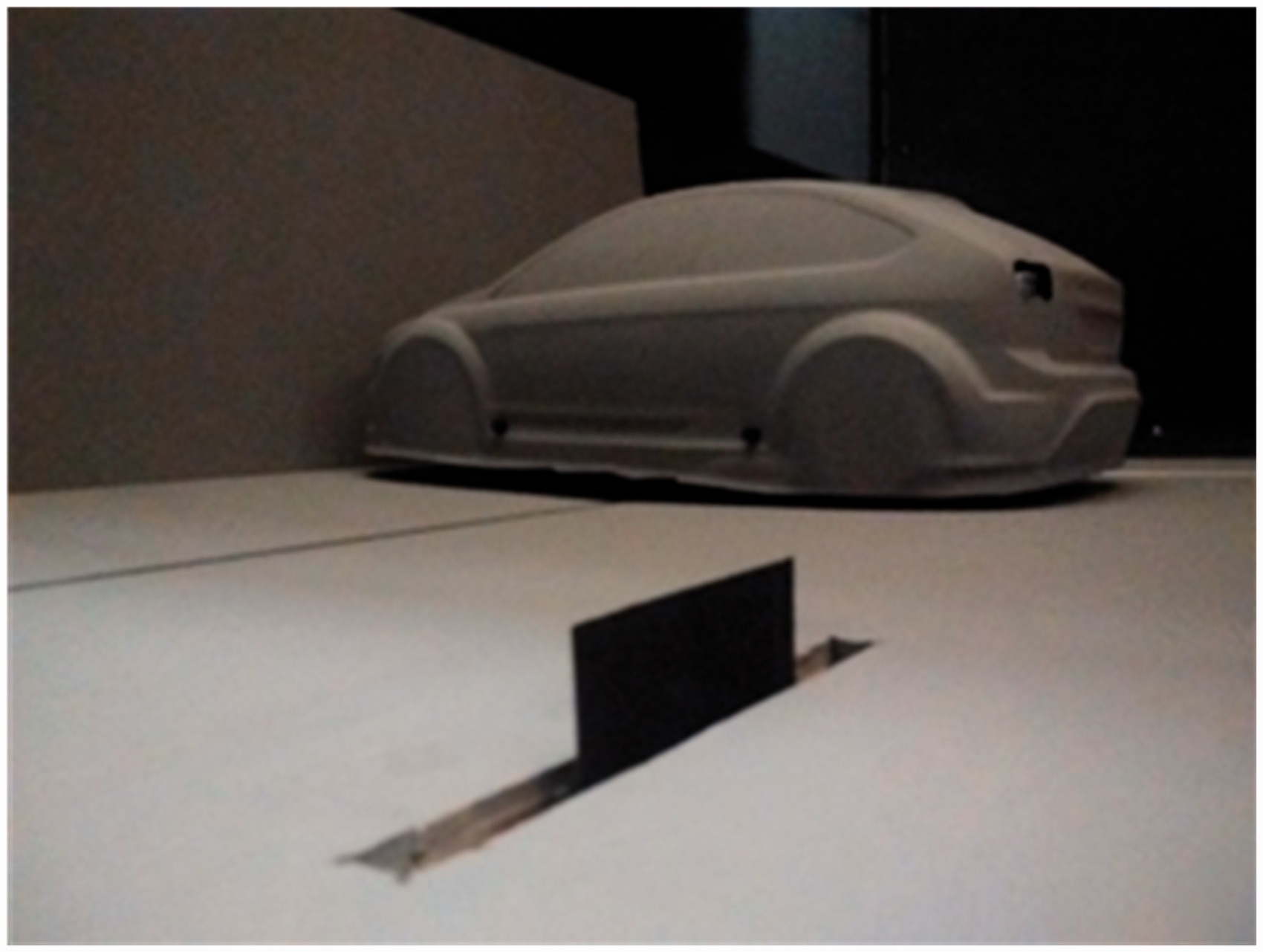

The second detection target represented an obstacle lying on the surface of the middle lane, scaled to represent a distance of 47 m ahead. The obstacle (a matt black rectangular vane) was normally out-of-sight below the surface of the road, but at random intervals was raised through a slot in the floor. At its full height of 20 mm, the 60 mm wide obstacle subtended the same visual size as a common tyre lying on its side. This subtended a visual size of approximately 0.25° × 0.75°. The obstacle rose to full height in 1 second, remained for 2 seconds, and then took 1 second to drop back out of sight. Participants were instructed to press the foot pedal as soon as they noticed the obstacle.

Luminance contrasts were calculated as C = (L_t − L_b)/L_b where L_t is the target luminance and L_b is the background luminance. The road obstacle was seen in negative contrast, with the vertical surface of the target darker than the surrounding road surface, with contrasts of C = −0.88 at 0.1 cd/m², and C = −0.96 at luminances of 1.0 cd/m² and 2.0 cd/m². A reason for these differences is that at the lower luminance, the contribution of the headlamps in lighting the vertical surface of the target is greater than at the higher luminances.

Participants saw the rear surface of the target vehicles. Due to these being scale models of real vehicles this presented a complex surface with three distinct regions – the bumper, tailgate and rear window, all three painted matt grey. The window luminance was higher than that for the bumper or tailgate, this being because while the bumper and tailgate were approximately vertical, the window was rotated towards horizontal. Note also that from the driver’s viewpoint, the bumper was surrounded by horizontal road surface, but the tailgate and window were seen against the rear vertical surface of the test chamber. The bumper presented a contrast of approximately C = −0.80 against the road surface, i.e. a negative contrast. The tailgate presented a positive contrast of approximately C = 0.7 against the side surrounds. The window contrast changed with luminance, being approximately C = 8.0 at 0.1 cd/m² and C = 12.0 at the higher luminances.

A dynamic fixation task was carried out in parallel to the detection tasks, with the purpose of placing the detection tasks in the driver’s peripheral visual field ¹³ and to simulate the non-static gaze patterns of a driver. The fixation target followed a random path within a 10° circle ¹⁴ with the lower fifth excluded to avoid it coming too close to the cars and obstacle. The target was between 6° and 12° above the horizontal sightline and the detection tasks (cars and obstacle) were between 0° and 2° below the horizontal. The cross presented a luminance of 1.3 cd/m² against the background luminance of 0.03 cd/m², as measured using a Konica-Minolta LS-110 luminance meter with no other light sources present. It subtended a visual size of 34–54 minutes arc at the viewing distance of approximately 5.1 m. This task required the participant to track the moving image of a cross projected onto the back wall of the chamber. At irregular intervals (from 1 to 6 seconds) the cross would be replaced for 300 milliseconds by a random number between 1 and 9. Participants read aloud the numbers and the experimenter recorded these responses. Reading accuracy was used as a measure of the degree to which fixation was maintained.

3. Procedure

Participants were seated at the apparatus, ensuring the foot pedal and steering wheel button positions were comfortable, before ambient room lights were switched off and a 20-minute adaptation period commenced. During adaptation, with the apparatus lighting set to the condition the participant would first experience, the experimenter explained the set-up. Participants were instructed to pay attention primarily to the dynamic fixation marker whilst simultaneously responding to the lane change and obstacle detection. They were asked to press the relevant response button/pedal when a detection event was noted, even if not completely sure that it was an event; the potential for false alarms was subsequently controlled by limiting the reaction time thresholds used to define a correct response. A practice trial was carried out to gain familiarity with the stimuli and response mechanisms.

In trials, there were three parallel tasks: (i) reading aloud the dynamic fixation digit when this momentarily changed from a crosshair; (ii) pressing the steering wheel button in response to a lane change by one of the cars ahead; and (iii) pressing the foot pedal in response to a suddenly appearing road surface obstacle. Reaction times were as measured from the onset of movement by the detection target to the participant pressing the steering wheel button/foot pedal as appropriate. To notify the participant that their response was acknowledged, their action was automatically followed by an electronic bleep. A recording of ambient sound inside a moving car was played throughout all conditions.

Presentation orders of the three detection targets (obstacle and two cars) were divided into one-minute bins. Within each bin there were four detection events, presentation of two lane changes (either car) and two surface obstacles. These were initiated at pseudo-random intervals randomly selected from between 5 and 26 seconds whilst ensuring that four events were completed in any one-minute period. No two events overlapped. The number of lane changes was balanced between the cars every two bins, so there were always two right and two left car lane changes every two bins.

The experiments examined four light settings (Table 1). For each light setting there were trials which started with the road lighting switched on for 4 minutes and then switched off for 20 minutes (an On–Off trial), and also the reverse transition with an initial 4 minutes with no road lighting and then 20 minutes with the road lighting switched on (an Off-On trial). This gave eight different test conditions. The order in which conditions were experienced was semi-randomised: an On–Off trial was followed by an Off-On trial (and vice versa) to reduce changes in adaptation between trials. Each trial lasted for approximately 25 minutes and each test participant attended 3 separate 2-hour test sessions to complete all 8 lighting conditions.

A sample of 30 test participants were recruited, drawn from 2 age ranges (younger: 18–30 years and older: 40–70 years) to allow an analysis of the effect of age (Table 2). Acuity was tested using a Landolt ring chart; participants wore corrective lenses for the acuity test and for the test trials if they usually wore them when driving. All test participants had a Snellen acuity of approximately 6/10 or better (equivalent to logMAR ≥ 0.20), which is the minimum requirement for driving in the UK. Colour vision examined using the Ishihara test (under a D65 source) did not suggest any test participants to have non-normal colour vision. Test participants were given a small reimbursement for their participation.

Table 2

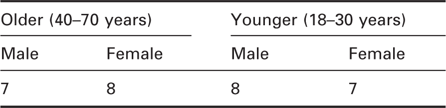
Age and gender breakdown of the test sample

Older (40–70 years)		Younger (18–30 years)
Male	Female	Male	Female
7	8	8	7

Note that for analysis of the reaction time data, for the obstacle, the available sample per lighting condition reduced from 30 to approximately 22 (range 19–25). This is because some test participants did not detect any of the obstacles under a particular condition and hence there were no reaction time data to analyse. In contrast, virtually all participants detected the car lane change at some point during the trial.

4. Results and analysis

The minimum reaction time for both car and obstacle targets was 500 ms; reaction times derived from previous research suggest faster genuine detection and reaction (pressing the button or pedal) is unlikely. ¹⁵ The maximum reaction time allowed for detection of the car was 6000 ms, this being the length of time the car took to move from the outside lane into the centre lane. The maximum reaction time allowed for detection of the obstacle was 4000 ms, this being the total length of time the obstacle was fully or partially visible, which included time to rise and descend. These threshold criteria resulted in the exclusion of 442 responses, representing 2.0% of all responses made. Note, for consideration of collision avoidance, that reaction times were measured from first onset of movement: for the first second following onset the obstacle was smaller than full size, representing the approach towards the same obstacle but at a greater distance. At 70 mph (113 km/h) the full-size obstacle would have been hit if not seen within 1.5 seconds. This overall detection time of 2.5 seconds matches the assumed time for detecting and perceiving hazards. ¹⁶

4.1. Main effects

The first stage of analysis was to compare the effects of age, light condition, whether the lights were on or off, and the stage of the trial. This comparison represented a 2 × 4 × 2 × 2 factorial model. Age was a between-subjects factor with two levels (Young and Old); Light condition was a within-subjects factor with four levels (Low S/P ratio, 1.0 cd/m²; High S/P ratio, 0.1 cd/m²; High S/P ratio, 1.0 cd/m²; High S/P ratio, 2.0 cd/m²); Lights on or off was a within-subjects factor with two levels (On and Off), and the stage of the trial was a within-subjects factor with two levels (Baseline or post-switch). These factors were used within linear mixed-effects models for each of the response variables and targets. Three of the four models showed normal distributions of residuals, as assessed by inspection of histograms and Q–Q plots. The residuals of the model for detection rates of the car showed signs of non-normality, but this was considered acceptable given that linear mixed-effects models are robust to small deviations from normality (e.g. Warrington et al. ¹⁷ ). Table 3 shows the results from each of these linear mixed-effects models.

Table 3

F statistics and p-values for detection rates and reaction times to each target

Effect	Car lane change				Obstacle
	Detection rate		Reaction time		Detection rate		Reaction time
	F	p	F	p	F	p	F	p
Age	0.14	0.71	0.28	0.60	16.6	<0.01**	1.84	0.19
Light condition	0.40	0.76	5.84	<0.01**	4.13	0.01*	8.51	<0.01**
Trial stage	7.48	<0.01**	4.98	0.03*	0.01	0.91	1.01	0.32
Lights On–Off	31.6	<0.01**	606	<0.01**	981	<0.01**	409	<0.01**
Age × light condition	0.17	0.91	0.97	0.41	0.87	0.46	0.61	0.61
Age × trial stage	0.15	0.70	0.22	0.64	0.47	0.50	2.06	0.15
Light condition × trial stage	0.95	0.42	0.12	0.95	0.68	0.57	1.75	0.16
Age × lights On–Off	5.52	0.02*	39.1	<0.01**	55.1	<0.01**	<0.001	0.98
Light condition × lights On–Off	0.26	0.85	6.23	<0.01**	1.27	0.28	6.12	<0.01**
Trial stage × lights On–Off	1.70	0.19	0.02	0.90	3.01	0.08	0.38	0.54
Age × light condition × trial stage	0.42	0.74	0.77	0.51	0.98	0.41	0.10	0.96
Age × light condition × lights On–Off	0.02*	1.00	1.68	0.17	1.66	0.18	1.79	0.15
Age × trial stage × lights On–Off	0.19	0.67	0.35	0.55	1.88	0.17	0.01	0.94
Light condition × trial stage × lights On–Off	2.09	0.10	0.61	0.61	2.16	0.09	1.29	0.28
Age × light condition × trial stage × lights On–Off	0.64	0.59	0.29	0.84	0.70	0.55	1.47	0.23

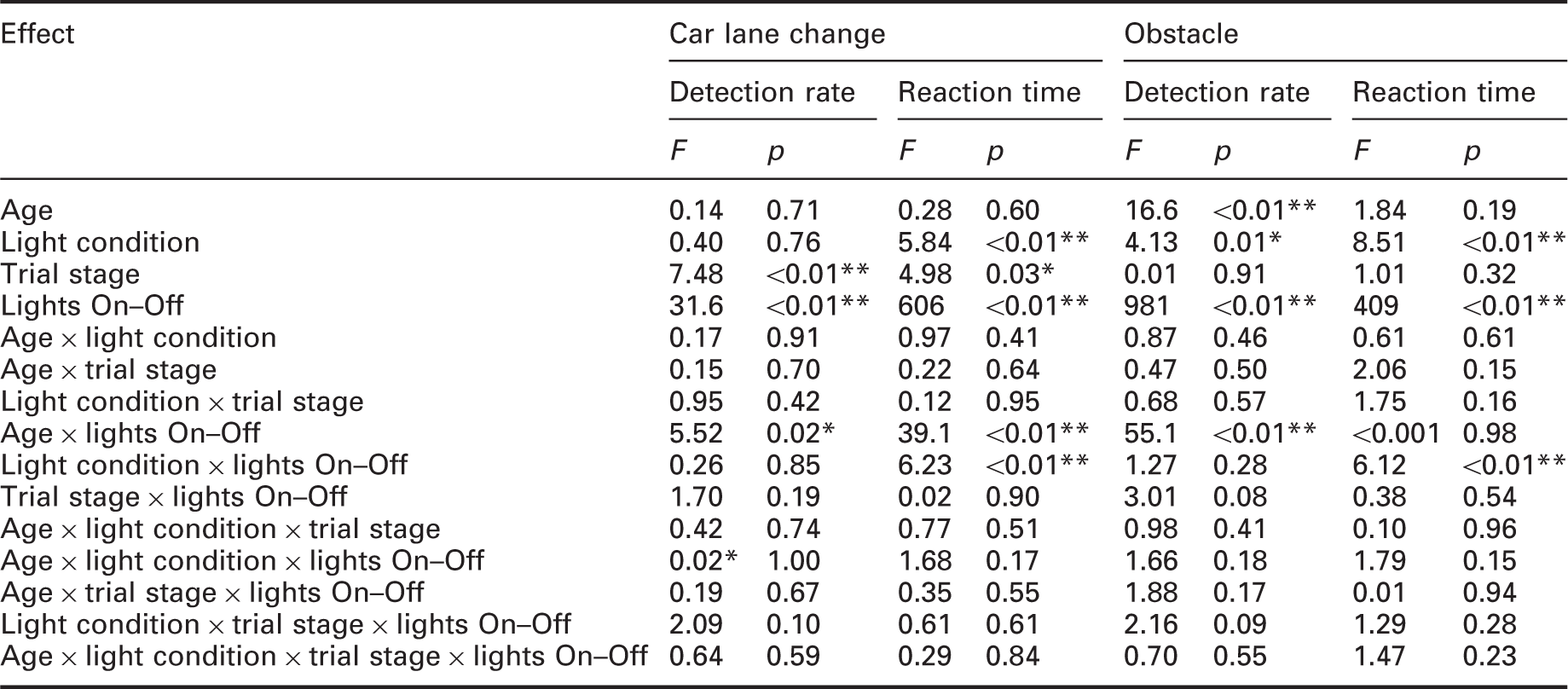
Results based on linear mixed models.

*

Statistically significant at p < 0.05.

**

Statistically significant at p < 0.01.

Figure 4 shows the mean detection rates for the lane change, for young and old participants under each combination of light condition, stage of the trial and whether the overhead lights were on or off. This does not show any obvious pattern of results, other than that detection rates for the car were near maximal performance under all combinations of conditions.

Figure 4.

Mean detection rates of car lane change for old and young participants, at each light condition, trial stage and whether the overhead lights were on or off. Error bars show the standard error of the mean. Note: The ‘off’ conditions show the mean as averaged across trials associated with all four lighting conditions.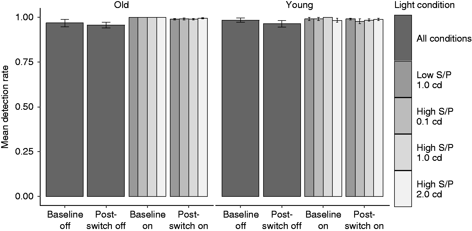

The only significant main effects revealed by the linear mixed-effects model were for the stage of the trial and whether the overhead lights were on or off. Detection of the car was slightly better during the baseline period (mean = 0.986) compared with the post-switch period (mean = 0.975). Detection rates were better when the lights were on (mean = 0.992) compared with when they were off, and only the headlights were on (mean = 0.969). The only interaction suggested by the model was between the age of the participant and the effect of the lights being on or off. This interaction is shown in Figure 5. The plot suggests that the older participants were affected slightly worse than younger participants when the overhead lights were off, but situation reversed when the lights were turned on. This was confirmed with post hoc Tukey’s tests, which showed that whilst the detection rates for older participants were significantly better when the overhead lights were on compared with off (p = 0.007), detection rates for younger participants were not significantly different between lights on or off (p = 0.59).

Figure 5.

Mean detection rate of car by age group and whether the overhead lights were on or off. Error bars show the standard error of the mean.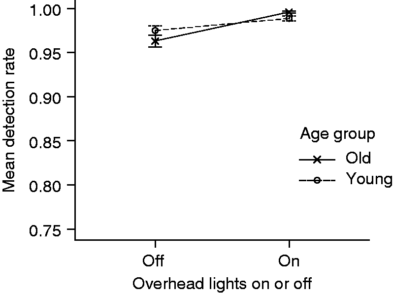

Figure 6 shows the mean detection rates of the obstacle, for young and old participants under each combination of light condition, trial stage and whether the overhead lights were on or off. There appears to be an obvious effect of age, with older participants having lower detection rates compared with the younger participants. There is also a clear effect of the overhead lights being switched on, this producing better detection rates. There may also be a suggestion of differences in detection rates between the light conditions, particularly with the high S/P at 0.1 cd/m² condition producing poorer detection rates than the other light conditions under many circumstances.

Figure 6.

Mean detection rates of obstacle for old and young participants, at each light condition, trial stage and whether the overhead lights were on or off. Error bars show standard error of mean.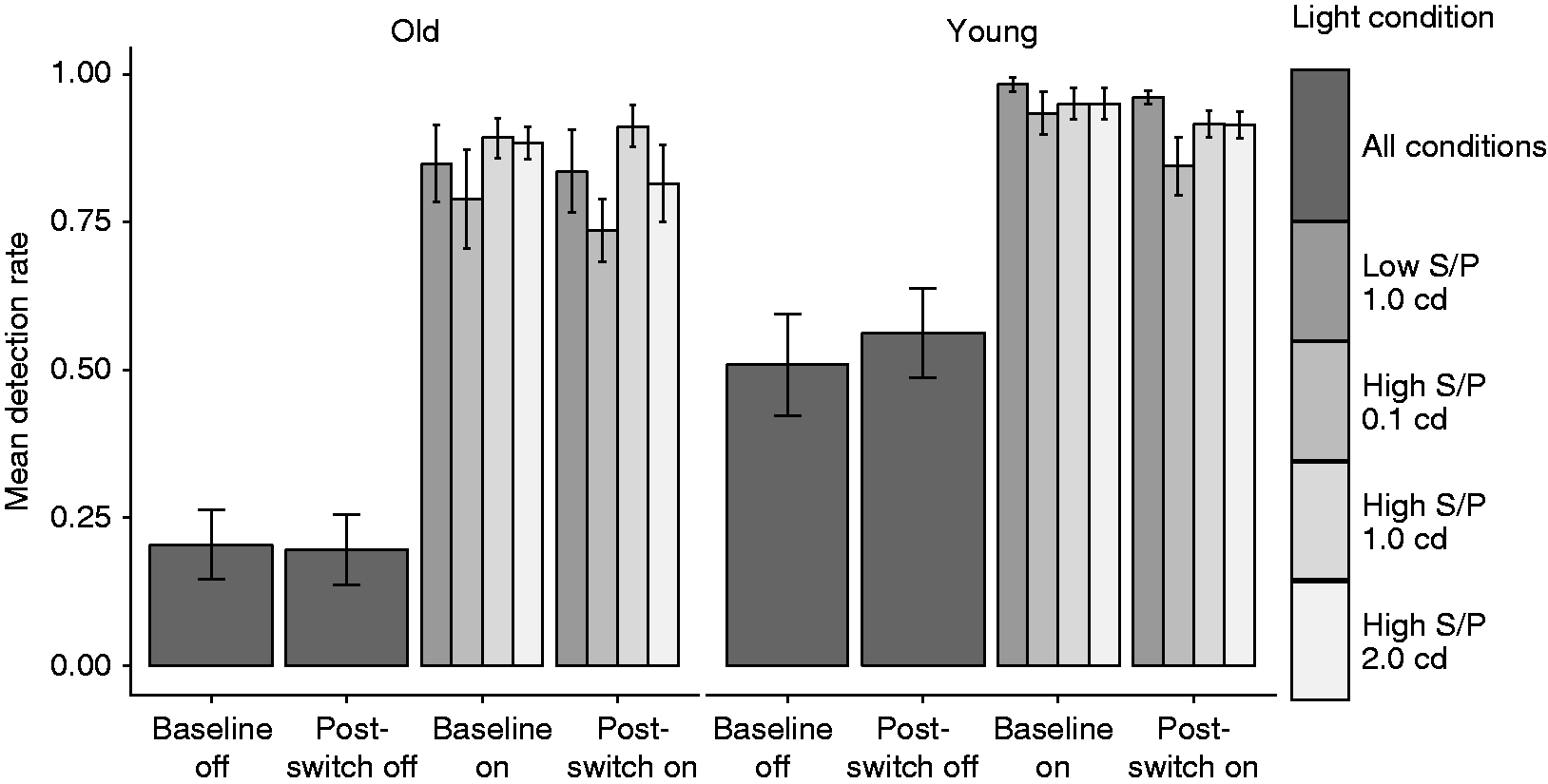

The linear mixed-effects model that compared detection rates for the obstacle found that there were significant effects for age of the participant, light condition and whether the overhead lights were on or off. Younger participants had significantly better detection rates (mean = 0.73) for the obstacle than older participants (mean = 0.52). To determine the effect of light condition on detection rates of the obstacle, post hoc Tukey’s tests showed that the high S/P, 0.1 cd/m² condition produced a significantly lower detection rate (mean = 0.83) compared with the high S/P, 1.0 cd/m² (mean = 0.92, p = 0.006) and low S/P, 1.0 cd/m² (mean = 0.91, p = 0.02) conditions. It was also close to being significantly different from the high S/P, 2.0 cd/m² condition (mean = 0.89, p = 0.10). The other light conditions did not differ from each other (all p-values > 0.76).The absence of overhead lights had a significant effect on detection of the obstacle, with detection rates being higher when the lights were on (mean = 0.89) compared with off (0.37). The only significant interaction was between the age of the participant and the effect of the overhead lights being on or off. This interaction is plotted in Figure 7. The plot suggests that the detection rates of the obstacle for older participants were more adversely affected when the overhead lights were off, compared with younger participants. This was confirmed by post hoc Tukey tests, which showed that detection rates for older participants were significantly worse than for younger participants when the overhead lights were off (p < 0.001), but there was no difference between the age groups when the lights were on (p = 0.49).

Figure 7.

Mean detection rate of obstacle by age group and whether the overhead lights were on or off. Error bars show the standard error of the mean.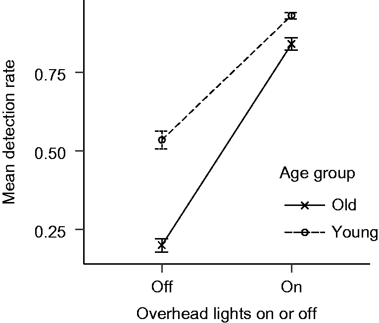

Figure 8 shows the mean reaction times to detection of the lane change for young and old participants, under each combination of the light condition, the stage of the trial and whether the overhead lights were on or off. Reaction times when the overhead lights were on are shorter than when the lights are off. There is also a suggestion that reaction times were shorter for the young participants but only when the overhead lights were off. The low luminance condition (0.1 cd/m²) consistently produced longer reaction times compared to the other three light conditions, when the overhead lights were on.

Figure 8.

Mean reaction times to detection of car lane change for old and young participants, at each light condition, trial stage and whether the overhead lights were on or off. Error bars show the standard error of the mean.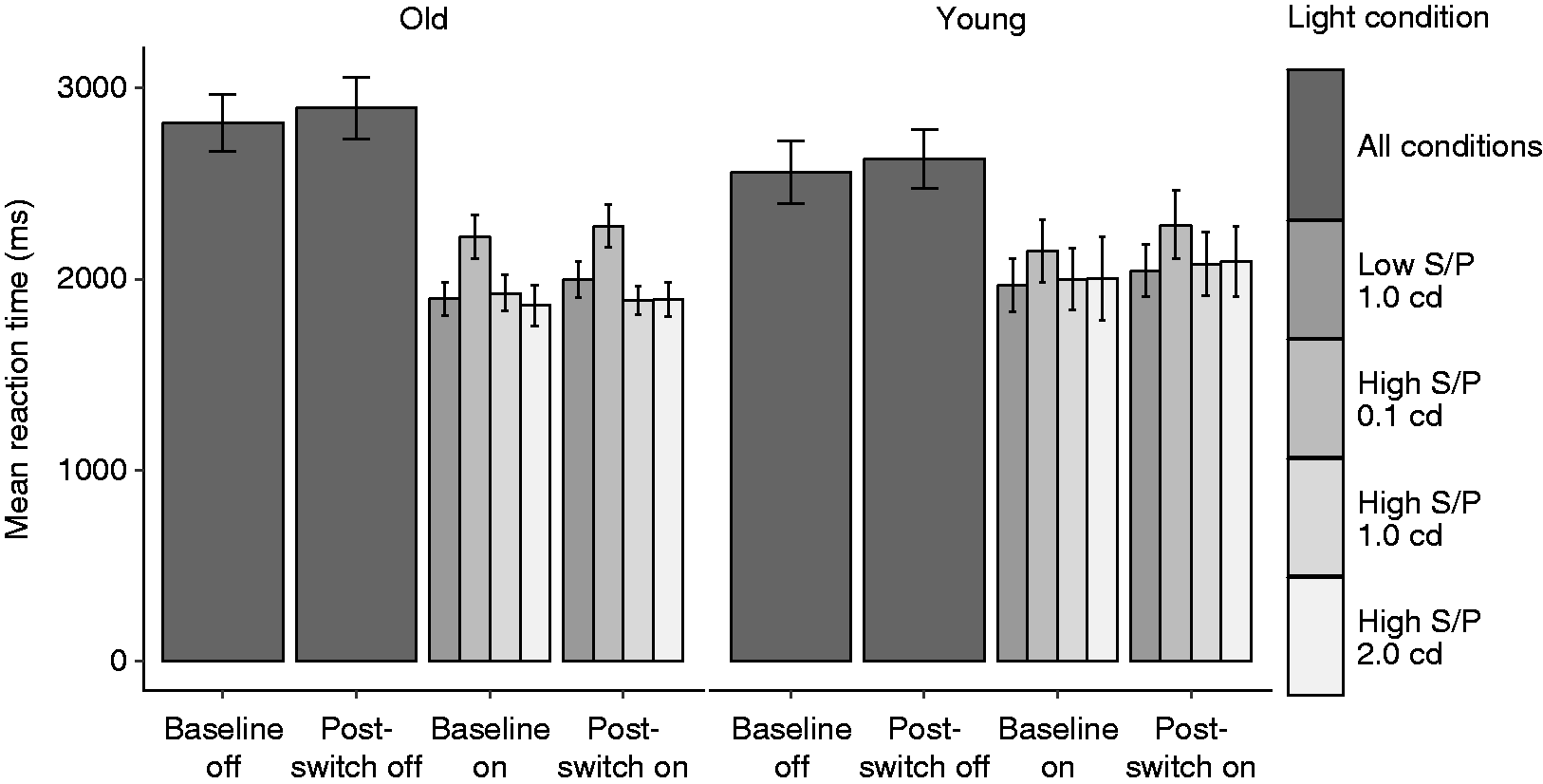

The main effects found by the linear mixed-effects model for reaction times to detecting the car were for the stage of the trial, the light condition and whether the overhead lights were on or off. The baseline period produced shorter reaction times (mean = 2347 ms) than the post-switch period (2410 ms).

Post hoc Tukey’s tests also showed that reaction times were significantly longer under the high S/P, 1.0 cd/m² lighting condition compared with the other three conditions (p < 0.001 in all three comparisons). This effect was obviously only apparent when the overhead lights were on, as confirmed by the interaction between light condition and the on–off status of the overhead lights. Having the overhead lights switched on produced significantly shorter reaction times to detecting the car (mean = 2034 ms) than when switched off (mean = 2722 ms). The presence of the overhead lights also interacted with the age of the participant, as plotted in Figure 9. The plot shows that the reaction times of older participants were affected more adversely when the lights were switched off compared with younger participants, but there was little difference between the two age groups when the lights were on. Post hoc Tukey’s tests were unable to confirm this interpretation, however.

Figure 9.

Mean reaction times to detection of the car by age group and whether the overhead lights were on or off. Error bars show the standard error of the mean.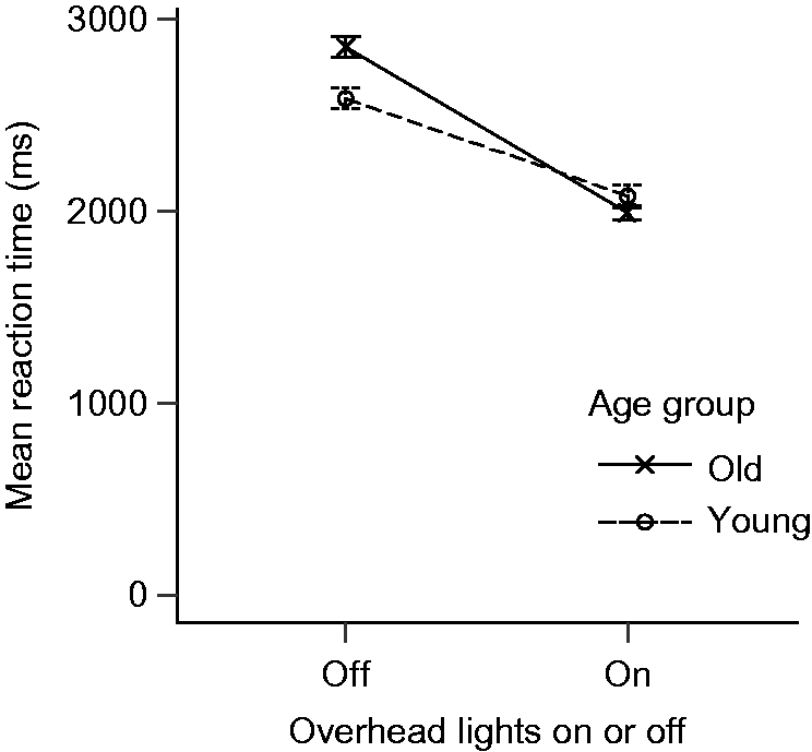

Figure 10 shows the mean reaction times to detection of the obstacle for young and old participants, under each combination of the light condition, the stage of the trial and whether the overhead lights were on or off. This again shows an improvement in reaction times when the overhead lights are on. There is a slight suggestion that younger participants may have had quicker reactions than older participants, particularly when the overhead lights were off. There also appears to be differences between the light conditions, specifically with the high S/P, 0.1 cd/m² condition producing slower reactions than the other light conditions.

Figure 10.

Mean reaction times to detection of obstacle for old and young participants, at each light condition, trial stage and whether the overhead lights were on or off. Error bars show the standard error of the mean.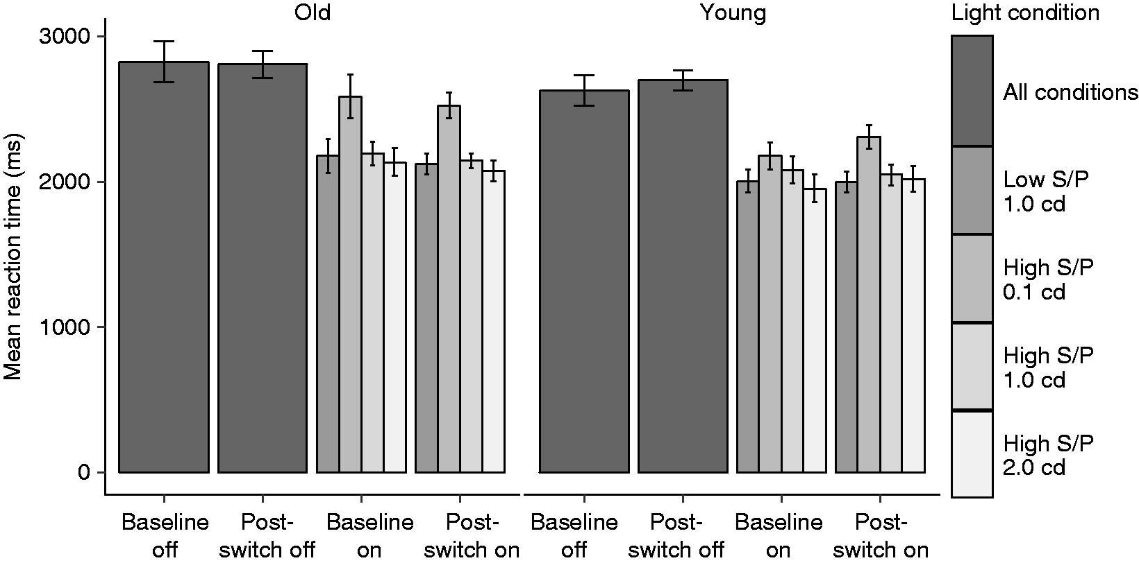

The linear mixed-effects model only found significant main effects for the light condition and whether the overhead lights were on or off. Post hoc Tukey’s tests confirmed that the high S/P, 0.1 cd/m² condition produced significantly longer reaction times to the obstacle (mean 2534 ms) compared with the high S/P, 1.0 cd/m² (mean = 2389 ms), high S/P, 2.0 cd/m² (mean = 2354 ms) and low S/P, 1.0 cd/m² (mean = 2346 ms) light conditions (all p-values < 0.001). None of the other light conditions significantly differed from each other (p-values all >0.37). This effect was only present when the overhead lights were on, as illustrated by the significant interaction between light condition and whether the lights were on or off (F(3,159) = 6.12, p < 0.001). No other interaction effects between the factors were statistically significant.

4.2. Performance post-transition

The aim of this experiment was to examine the effects of transition between lit and unlit sections of road, simulated in this work by switching on or off the overhead lighting. A baseline period of 4 minutes, in which the overhead lights were either on or off, was followed by a 20-minute period in which the status of the overhead lights was reversed from the baseline period.

Vertical illuminances at the participant’s eye were measured; these were 0.01 lux for head lighting only, 0.11 lux with road lighting of nominal luminance 0.1 cd/m² and 0.95 lux for nominal luminance of 1.0 cd/m². For changes within 2–3 log units, neural adaptation is sufficient and takes place within 200 ms. ⁷ If photochemical adaptation was also involved, then the adaptation response would take longer, a period of several minutes.

Mean values for 4-minute periods during each trial have been calculated, and are plotted in Figures 11 and 12. Figure 11 shows the mean detection rates for each target, light sequence and light condition, and Figure 12 shows the same information but for mean reaction times. These plots illustrate the change in detection performance when the overhead lights are switched on compared with switched off, with the exception of the detection rates for the car, which remained near maximal performance regardless of whether the lights were on or off. The plots also highlight again the slightly poorer detection performance given by the low luminance (0.1 cd/m²) condition compared to the other light conditions.

Figure 11.

Mean detection rates per 4-minute period of the trial, by target, light switch sequence and light condition. The vertical lines indicate when the overhead lights were switched.

Figure 12.

Mean reaction times per 4-minute period of the trial, by target, light switch sequence and light condition. The vertical lines indicate when the overhead lights were switched.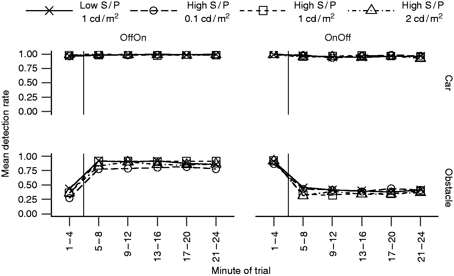

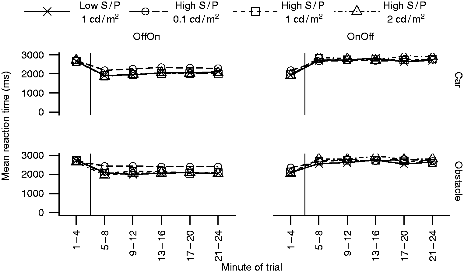
Figures 11 and 12 do not suggest any long-term changes in performance, after the switch, as might occur due to adaptation, with performance following a relatively steady level throughout the 20-minute period.

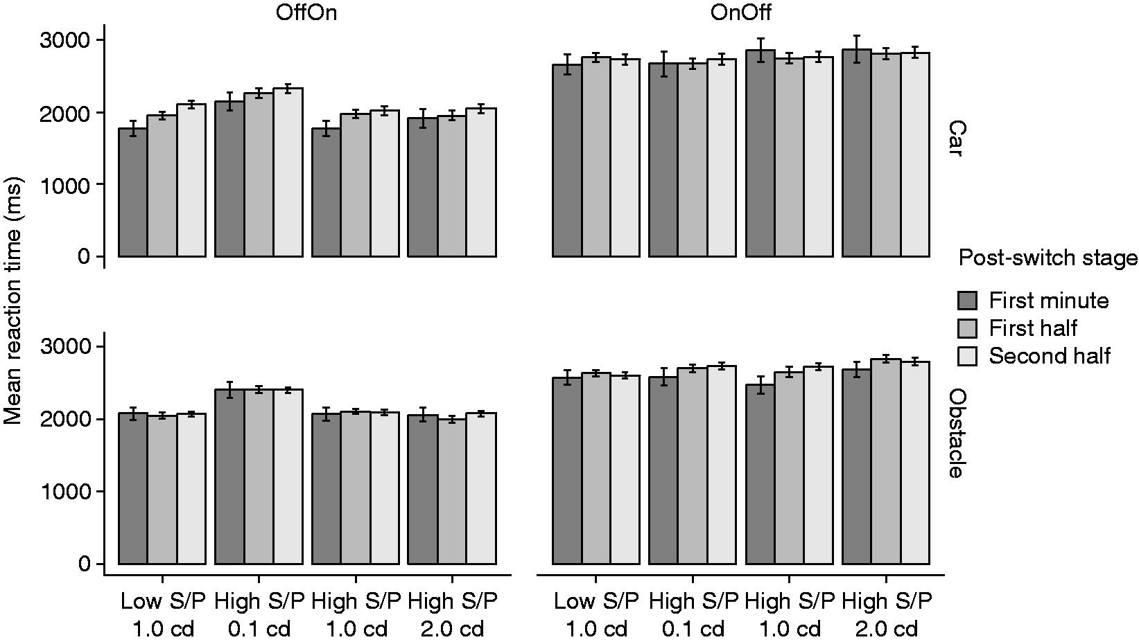
This analysis was carried out using data across a four-minute interval, and it is possible that this hides a change in the immediate post-switching interval. Further analysis was carried out by comparing detection performance in this first minute of post-switch period (the fifth minute of the trial overall) against performance in the remainder of the first half of the post-switch period (minutes 6–14 of the trial) and in the second half of the post-switch period (minutes 15–24 of the trial). The detection rates for these three stages of the post-switch period by the target, light switch sequence and light condition are shown in Figure 13. The reaction times are shown in Figure 14.

Figure 13.

Mean detection rates for detection of car and obstacle, by light-switch sequence, light condition, and stage of the post-switch period. Error bars show the standard error of the mean.

Figure 14.

Mean reaction times for detection of car and obstacle, by light-switch sequence, light condition, and stage of the post-switch period. Error bars show the standard error of the mean.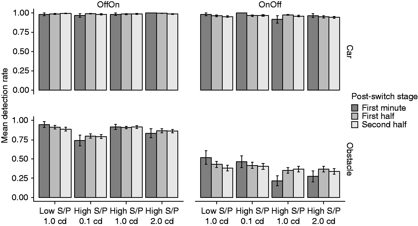

Linear regression models were carried out to test whether there were any significant differences between the post-switching stages or any significant interactions with the light condition under each of the different conditions. The results of these models are shown in Table 4. These suggest that the only main effect of the post-switch stage was for reaction times to the car lane change task: post hoc Tukey’s tests confirmed that the first minute of the post-switch period produced significantly shorter reaction times (mean =1903 ms) than the rest of the first half (mean = 2030 ms) and the second half (mean = 2121 ms) of the post-switch period.

Table 4

F and p values from linear regression models, comparing mean detection rates and reaction times to targets during the different stages (first minute, first half and second half) of the post-switch period

Light switch sequence	Effect	Car lane change				Obstacle
		Detection rate		Reaction time		Detection rate		Reaction time
		F	p	F	p	F	p	F	p
Off–On	Post-switch stage	0.48	0.62	19.6	<.01*	0.28	0.76	0.05	0.95
	Light condition × post-switch stage	0.52	0.79	0.98	0.44	1.06	0.39	0.20	0.98
On–Off	Post-switch stage	0.15	0.86	0.05	0.95	0.50	0.61	1.68	0.19
	Light condition × post-switch stage	1.65	0.14	0.53	0.79	4.12	<.01*	0.31	0.93

*

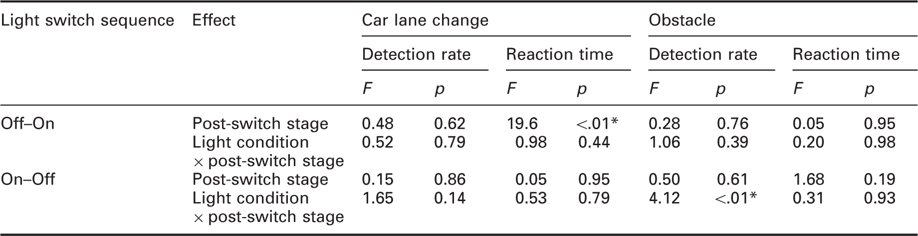
Statistically significant at p < 0.01.

5. Discussion

5.1. Internal validation

A series of validation checks were carried out to confirm whether the experiments provided consistent, reproducible and reliable results. One of the key premises of the study was that the tasks of detecting the car lane change and obstacle were carried out using peripheral rather than foveal vision. A dynamic fixation marker was used to engage foveal vision and place the target area in the peripheral vision of the participant. Previous work using eye-tracking has shown that such a dynamic fixation marker can be highly successful at maintaining foveal gaze. ¹³ The success rate of correctly identifying fixation marker each time it changed to a digit also provides an indication of how effectively the marker maintained the foveal gaze of participants during the current study. A high success rate would provide reassurance that peripheral vision was being used for the detection tasks, as it would be highly unlikely the fixation marker digit could be identified without foveal vision being used, ¹⁸ given its relatively small size, brief presentation time, and unpredictable movement.

The mean rate of correct identification of the fixation target during the experiment reported in this article was 89.7% (sd =9.5%). The identification rate in the fog experiment that was run in parallel with this study ⁹ was 93.6% (sd = 4.6%) during trials with no fog and 93.4% (sd = 5.5%) during trials with thin fog. However, the rate dropped to 80.7% (sd = 12.5%) during trials with thick fog. This decrease in identification of the fixation target is however expected, as the visibility of this target was reduced due to the increase in fog density.

These fixation target identification rates are high, and similar to the 98% rate found by Fotios, Uttley and Cheal ¹³ using a similar dynamic fixation task, who also demonstrated by recording gaze direction using eye tracking apparatus that fixation was maintained on the fixation target during the task. We therefore conclude that in order to achieve these high success rates participants tended to maintain their foveal gaze on the fixation target, and therefore the task of detecting the car lane change and obstacle consistently used peripheral vision.

Comparison of the detection and reaction time results from equivalent conditions in the current transition experiment and the parallel fog experiments allows verification of the repeatability and consistency of results obtained using the experiment’s apparatus. Specifically, the ‘No fog’ condition of the fog experiment ⁹ was equivalent to the baseline period of the transition experiment during ‘On–Off’ trials, i.e. when the overhead lights were on during the baseline period. Three light conditions were used in both experiments: 0.1 cd/m² and 1.0 cd/m² at S/P = 1.4 and 1.0 cd/m² at S/P = 0.65. Figure 15 compares the reaction times to detection for the fog and transition experiments under these three light conditions.

Figure 15.

Mean reaction to detection for fog (No fog condition) and transition (baseline period, overhead lights on) experiments, for three comparable light conditions. Error bars show the standard error of the mean.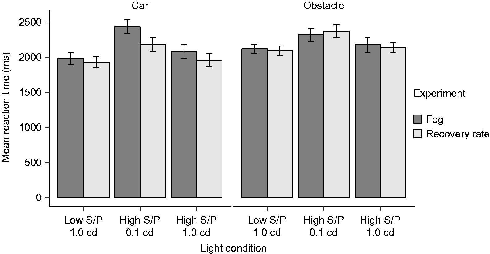

Figure 15 suggests some possible differences between the two experiments for the same comparable light condition. For example, reaction times were shorter during the transition trials in five of the six light conditions. However, linear mixed effects models for each target and response measure did not suggest any differences between the two experiments to be significant (see Table 5).

Table 5

Comparison of mean overall responses during fog and transition experiments for each target and response variable

Target	Response measure	Mean overall response a		Significance of difference between experiments (p-value)
		Fog experiment	Transition experiment
Car	Detection rate	0.99	0.99	0.19
	Reaction time (ms)	2165	2023	0.41
Obstacle	Detection rate	0.76	0.90	0.12
	Reaction time (ms)	2204	2198	0.96

a

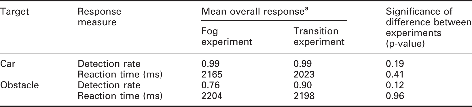
Mean overall response is the mean taken across all three light conditions.

A final confirmation of the reliability of the study results is illustrated by the consistency of performance in the transition experiment during the baseline period of Off-On trials and post-switch period of On–Off trials, and vice versa (Figures 11 and 12). For example mean detection of the obstacle during the baseline period of Off-On trials, when overhead lights were off (mean detection rate across all four light conditions = 0.36) were similar to the detection rate during the post-switch period of On–Off trials, again when overhead lights were off (mean detection rate across all four light conditions = 0.38). Mean reaction times were also similar between baseline and post-switch periods during equivalent light-switch conditions. For example, mean reaction time to detecting the obstacle during the baseline period of On–Off trials, when overhead lights were on, was 2164 ms, compared with 2155 ms during the post-switch period of Off-On trials, when overhead lights were also on.

5.2. Implications

There was a very clear effect of the presence of the overhead lights – detection rates and reaction times to detection for both the car and obstacle were significantly improved when the overhead lights were on compared with off. Detection rates improved from 0.97 to 0.99 for the car lane change, and from 0.37 to 0.89 for the obstacle. Reaction times improved (i.e. decreased) from 2722 to 2034 ms for the car lane change, and from 2728 to 2156 ms for the obstacle. The presence of overhead lights produced a greater improvement in detection performance amongst older participants compared with younger participants. This is in line with expectations, as visual performance deteriorates with age and this is most likely to be evident when the visual system is operating near its limits. ⁷ With no overhead lights on, the participants’ visual system was operating closer to threshold compared with when the overhead lights were on, and this helps explain why older participants were more adversely affected with the lights off. These findings suggest that the presence of road lighting in real driving situations can improve a driver’s chances of detecting a car changing lanes or an obstacle in front of them, and reacting more quickly to such a potential hazard. The improvement in reaction times provided by overhead lighting would reduce the required braking distance to a hazard in the road by 18 m, assuming a speed of 70 mph (113 km/h). Road lighting may be particularly beneficial to older drivers, whose detection and reaction capabilities are likely to be particularly reduced under darker conditions.

One question that remains is how much light should be provided by road lighting to obtain its beneficial effects. Detection performance was significantly improved by the presence of the overhead lights even at the lowest luminance of 0.1 cd/m², suggesting this luminance is better than no overhead lighting. Increasing the luminance to 1.0 cd/m² improved detection further, but increasing from 1.0 to 2.0 cd/m² did not produce any further improvements, which may be because the difference in luminance was too small to reveal a change in detection performance or because a plateau level of visual performance has been reached. This might suggest that having road luminances above 1.0 cd/m² may not provide any benefit in terms of enabling the driver to detect and avoid potential hazards in the road, but it should be noted that this conclusion is based on the experiment and its controlled conditions. Further work is required to confirm whether this conclusion applies in real-world settings.

The experiment included light conditions with two different S/P ratios (0.65 and 1.4) at a comparable luminance level (1.0 cd/m²). These different S/P ratios did not produce any significant differences in detection rates and reaction times to the two types of target. One reason for this may be because at that luminance level, a plateau in performance had been reached, meaning the spectrum of the light was unlikely to make a difference to the participants’ responses. Effects of spectrum are more likely to become apparent when the task is more difficult and when the luminance is lower. Previous work also failed to find any effects of spectrum at 1.0 cd/m².^19,20 The spectrum of the light may have a greater influence over the detection abilities of a driver at luminances below 1.0 cd/m².

A goal of the transition experiment was to investigate how detection performance changed following a sudden transition between lit and unlit sections of a road. The results showed that whilst there was a clear change in performance immediately following the transition in lighting, this level of performance then remained fairly constant with no apparent subsequent shifts over the course of the 20-minute post-switch period (Figures 11 and 12). We also examined for changes in participants’ detection performance following the abrupt switch in overhead lighting that occurred only within the first minute of the post-switch period. To do this, detection rates and reaction times during the first minute of the post-switch period were compared against the rest of the first half, and the second half of the post-switch period (Figures 13 and 14). This comparison did not indicate any obvious and consistent differences between performance in the first minute, immediately after the switch in light conditions, and the rest of the post-switch period.

In this work, the obstacle was more difficult to detect than a lane change. In the real world, vehicles tend to use rear lights which would further increase the detection of a lane change, with the potential to further exaggerate this difference.

6. Conclusion

These data suggest that when a driver moves from a lit to an unlit section of road, their detection performance decreases near-immediately to that expected for the conditions of the unlit section and that there is no significant subsequent increase in the following 20-minute period. Similarly, when driving from an unlit to a lit section, there is a near-immediate increase in detection performance that does not change with time.

Adding a small amount of road lighting (0.1 cd/m²) improved detection compared with no road lighting: increasing the luminance to 1.0 cd/m² improved detection further still but an additional increase to 2.0 cd/m² did not suggest further benefit. There was no difference in detection performance between S/P ratios of 0.65 and 1.40, both being examined at a luminance of 1.0 cd/m². These results suggest that, in the current context, visual performance reached a plateau at 1.0 cd/m².