
Abstract
This work presents a novel spatio-temporal InSAR (ST-InSAR) framework that integrates physics-based structural models into persistent scatterer interferometry (PSI) for bridge monitoring. The proposed approach mitigates the limitations of conventional PSI in civil infrastructure applications, namely large displacements that exceed the ambiguity limits, and absence of correlation with air temperature. ST-InSAR exploits spatial correlation among PSs to jointly estimate the displacements across the entire structure. The framework is applied to the Colle Isarco Viaduct (Italy), where its performance is compared with conventional multitemporal PSI, using benchmark topographic measurements. Results show that ST-InSAR detects structural displacements with an accuracy on the order of 2 mm, even where PSI fails. Additionally, temporal coherence increases from approximately 0.08 (PSI) to over 0.9. Finally, the framework enables the estimation of the temperature gradient across the bridge deck with an accuracy better than 1°C, providing information about the structural thermal state beyond displacement monitoring.
Introduction
Structural health monitoring (SHM) of bridges and viaducts is traditionally performed with contact-sensors directly installed on the structure of interest. Recourse to these technologies requires high economic investments, including the initial sensor costs, the installation and the maintenance.1,2 As a consequence, the number of infrastructures that can be equipped with continuous monitoring systems remains limited. This condition is particularly problematic in regions with large stocks of aging bridges, where widespread monitoring is promptly needed but conventional SHM strategies are impractical. 3 Practitioners and researchers have progressively shifted attention toward remote-sensing alternatives, 4 which do not require any physical intervention on the structure and can overcome the scalability issues inherent to contact-based approaches. Among these, synthetic aperture radar (SAR) has emerged as a powerful solution for large-scale infrastructure monitoring. SAR is an active microwave imaging technique capable of acquiring high-resolution images of the Earth’s surface. Operating from space or ground, SAR sensors illuminate the target surface and measure the backscattered signal, which is characterised by its amplitude (reflectivity) and phase. Because satellite acquisitions cover wide areas at regular intervals – usually one acquisition per 12–16 days for each satellite – SAR enables simultaneous monitoring of networks of infrastructures. 5 Moreover, SAR data are relatively inexpensive, with image costs ranging from free (e.g. from open-access missions such as Sentinel-1 6 ) up to a few thousand USD for ultrafine-resolution commercial products. 7
Within SAR-based methods, multitemporal interferometric SAR (MT-InSAR) exploits the phase difference between multiple SAR images acquired over the same target and detects slow displacement over time. 8 One widely applied MT-InSAR technique is persistent scatterer interferometry (PSI), which was first introduced by Ferretti et al. 9 and subsequently refined in numerous studies and comprehensively reviewed by Crosetto et al. 10 PSI focuses on pixels that behave as stable radar reflectors – typically metallic or geometrically sharp-like features – and extracts their displacement time series along the radar line of sight (LOS) with millimetric precision. PSI have been successfully employed for the monitoring of reinforced11,12 and prestressed concrete bridges,13,14 railway bridges,15,16 cable-stayed bridges,17,18 arch bridges, 19 dam foundations 20 and even scour-related processes. 21
Despite its advantages, PSI performance significantly depends on the temporal stability of the pixel amplitude and phase. Candidate persistent scatterers (CPS) are typically selected based on the amplitude stability index and later validated using temporal coherence, which quantifies how well a pixel phase time series follows the assumed interferometric phase model. However, several factors can lead to coherence loss, including
22
: changes in the scatterer properties (i.e. temporal decorrelation); changes in the orbit geometries (i.e. geometrical decorrelation); errors in the assumed deformation model; and displacements exceeding the radar measurement ambiguity interval. Because the interferometric phase is wrapped within the interval
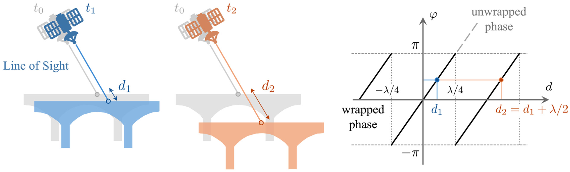
Phase ambiguity issue in which two bridge LOS displacements
Several methods have been developed to deal with poorly coherent persistent scatterers (PSs), such as Quasi-PS 24 and the Stanford Method for persistent scatterers (PSs). 22 These techniques perform well for several classes of problems, including land deformation monitoring, as long as the monitored displacements are slow (i.e. limited magnitude between satellite passes) and exhibit strong correlation with time and air temperature. In contrast, bridge displacement presents different characteristics:
In terms of magnitude, differential displacements between successive acquisitions can be large – especially for medium and long-span bridges – and may exceed the unambiguous displacement limit
Bridge displacements are not directly correlated with air temperature but rather with the structural temperature of the bridge, which is often governed by temperature gradients across the deck.
Another important limitation of conventional interferometric methods is that scatterers are treated independently, which inherently implies no spatial correlation between closely spaced points. This assumption is particularly limiting for bridge monitoring, where scatterers should exhibit space-correlated displacement given by the mechanics of structural deformation. Consequently, a natural extension of the InSAR techniques is to integrate into the analysis a physics-based model capable of predicting the spatial deformed shape of the structure of interest.
Physics-augmented approaches have been integrated with InSAR data regarding geotechnical and tunnelling applications to help resolve phase ambiguities.25–28 Regarding bridge monitoring, several studies have integrated structural models to interpret observed displacement patterns, solve phase-ambiguity issues, and infer potential material changes and damages.18,19,29–33 However, in these cases, bridge models were employed in a post-processing phase, once InSAR displacement measurements were already available.
To the best of the authors’ knowledge, no prior work has integrated a physics-based structural deformation model directly into the PSI extraction process itself in order to account for refined spatial and temporal bridge behaviour during the displacement time series estimation.
Research objectives
This article proposes a novel framework that directly integrates a physics-based structural model of the bridge into the interferometric phase formulation of PSI, explicitly accounting for spatial and temporal deformation. This integration is achieved by relaxing some conventional PSI assumptions, specifically the linear correlation of deck displacement with time and with air temperature, and by introducing spatial dependency of the PSs located on the bridge deck, according to the expected and compatible structural deflection.
The proposed framework is able to recover displacement information at locations that are typically discarded due to low temporal coherence. By mitigating the factors that typically lead to coherence loss in InSAR bridge monitoring, the method improves the reliability of displacement time series estimates that would normally be rejected. More specifically, it reduces displacement estimates errors and enhances the temporal coherence of PSI discarded pixels
This methodology is applied to the Colle Isarco Viaduct in Vipiteno (Italy), a long-span prestressed concrete highway bridge consisting of two parallel decks with cantilever–Gerber beam structural configurations. The results are compared with those obtained using conventional PSI and validated against benchmark topographic surveying measurements on the bridge.
The remainder of the article is organised as follows: the second section reviews the fundamentals of InSAR and the conventional PSI technique; the third section describes the proposed methodology; the fourth section presents the case study; the fifth section illustrates the results and compares the performance of the proposed framework with that of PSI. This is followed by an in-depth discussion in the sixth section and by the conclusions of the study in the seventh section.
SAR background
This section briefly revisits the fundamental concepts of SAR interferometry required to understand the methodology proposed in this work, with particular emphasis on the PSI technique. The objective is to introduce the key principles, assumptions, and processing steps underlying traditional PSI, in order to clarify its limitations when applied to bridge monitoring and to provide the motivations for this study.
In the remainder of this article, the term PSI refers to the traditional PSI approach.
SAR interferometry
In SAR imaging, the sensor emits a radar signal with an incidence angle
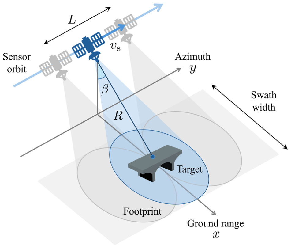
SAR geometry orbit in stripmap acquisition mode. SAR: synthetic aperture radar.
A displacement
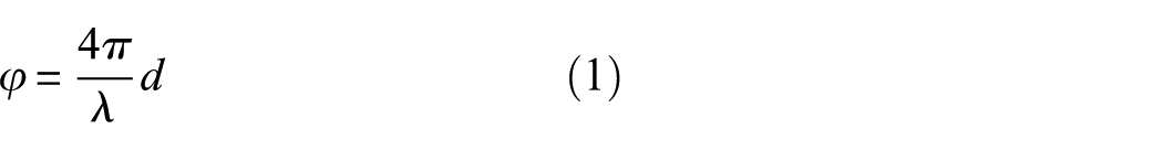
where
Given a reference acquisition
where
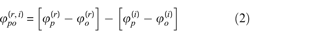
The interferometric phase

where
The contributions
The first term describes the sensitivity of the interferometric phase to the scatterer height
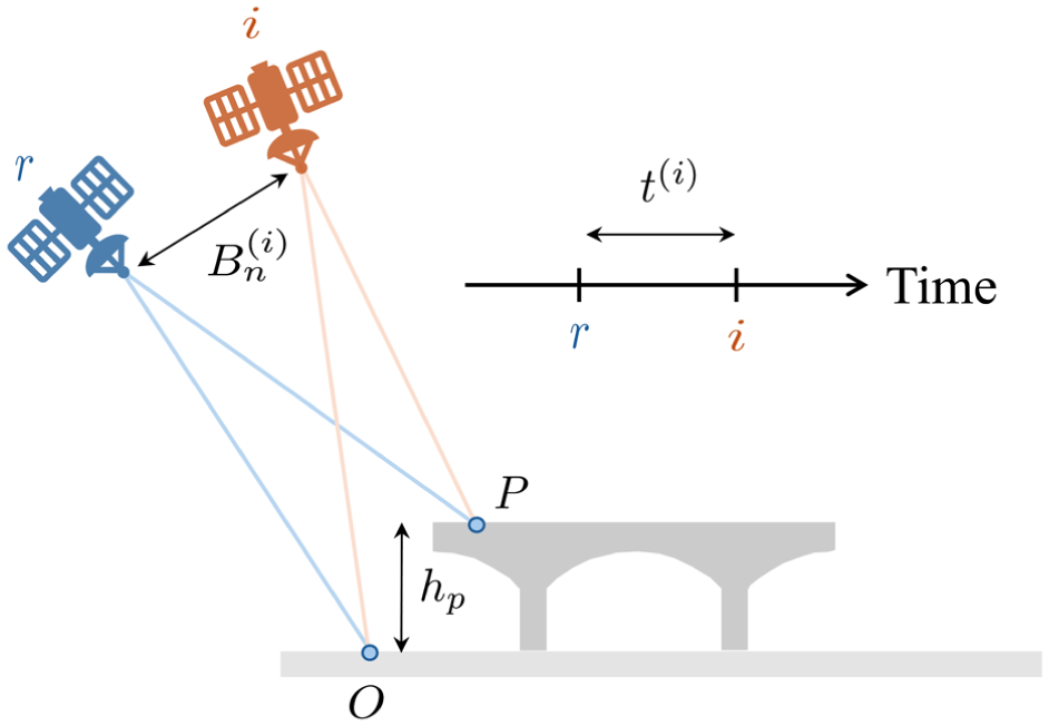
Interferometric geometry showing the reference orbit and the acquisition orbit at time
Multi-temporal InSAR and PSI
Multi-temporal InSAR uses a set of SAR acquisitions to reconstruct the entire time series of LOS displacement.
9
Let

where
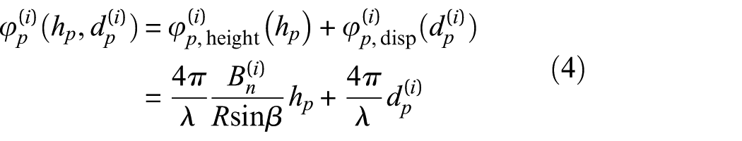
By substituting the displacement model in Equation (4), the interferometric phase can be written as a function of the scatterer height and the displacement coefficients:

where
The three unknown parameters
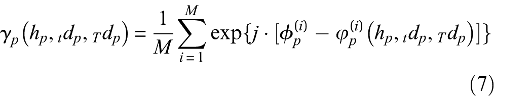
where
The optimal parameter estimates are obtained by maximising the magnitude of the objective function:
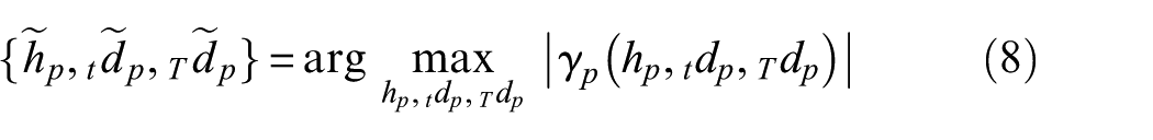
Once the optimal parameters are determined, the displacement time series for each PS can be reconstructed by substituting the optimal values
Finally, the temporal coherence
where, in this case, the subscript t is written on the right and in roman font to denote temporal coherence, rather than a time derivative. The pixel (i.e. CPS) is typically accepted as a permanent scatterer if its temporal coherence exceeds a certain threshold (usually preferably higher than 0.75 35 ).
PSI limitations in bridge monitoring
In summary, conventional PSI techniques approximate the behaviour of each persistent scatterer using a parametric displacement model assumed to be a linear function of time and air temperature, and spatially uncorrelated between neighbouring pixels. While these assumptions are often acceptable for monitoring slow-moving geophysical phenomena, they are often violated in the case of bridge monitoring, leading to a loss of performance.
The main limitations can be summarised as follows:
Long-span bridges often exhibit relatively large displacements that can exceed in magnitude the ambiguity limit
The assumption of spatially independent PSs is generally not valid for bridges, where closely spaced scatterers are mechanically dependent and must follow physically admissible deformation shapes given by the structural behaviour of the bridge.
Thermal deformation is governed by structural temperature, which is influenced not only by air temperature but also by solar radiation and thermal gradients. While the deformation of some structural components (e.g. piers or deck longitudinal expansion) may be primarily correlated with air temperature, other deformation mechanisms (e.g. deck deflection induced by vertical temperature gradients) cannot be adequately described using the above model.
As a consequence of these limitations, even pixels with stable reflectivity across all SAR acquisitions may result in having low temporal coherence and end up being discarded by conventional PSI analyses.
The methodology proposed in the next section addresses these limitations by jointly processing all stable scatterers, including those that would normally be discarded due to low temporal coherence, and by explicitly accounting for the physical behaviour of the structure.
Method
The general idea of the proposed framework is to employ, within the InSAR processing pipeline, a time-varying geometrical model that describes the expected structural deformation of the bridge. This key step allows one to constrain the space of admissible solutions to a limited set of physically feasible configurations, consistent with the expected spatial and temporal deformation behaviour of the structure. For this reason, the proposed approach is referred to as spatio-temporal InSAR (ST-InSAR).
In this section, the general ST-InSAR framework is presented, first describing the structural model employed and then illustrating its integration into the PSI analysis. Its application to a real-world case study is discussed in the fourth section.
Structural model
The first step consists in defining a structural model of the bridge – specifically the deck – to capture the spatial deformation affecting different PSs. This model replaces the generic deformation law of Equation (5), and explicitly describes the physical mechanisms responsible for the observed displacement. Defining a structural model can be done with several layers of approximations, ranging from simplified one-dimensional (1D) beam finite-element representations to more detailed shell or full three-dimensional (3D) models. Regardless of the chosen complexity, the deck deformation is mainly influenced by the following effects:
Permanent and live loads, that generate an elastic deformation, mostly vertical (Figure 4(a));
Temperature, that generates an expansion along the deck direction, expansion of the piers and vertical deflection (Figure 4(b));
Slow phenomena, such as creep or prestressing relaxation, affecting both vertical and horizontal displacements (Figure 4(c));
The unknown quantities that represent the deformation mechanisms listed above are collected in the vector
Illustration of some of different causes of bridge deformation: (a) dead load
The structural model uses known quantities such as time
where
Scheme of the reference system adopted to describe the 3D deck displacement. 3D: three-dimensional.
A further assumption, which covers the vast majority of practical cases, is that the SPs controlling the model can be classified into two groups:
Time-varying and space-constant parameters, for example, a temperature gradient
Space-varying and time-constant parameters, for example, a linear deformation rate or thermal expansion coefficient that differs from pier to pier but remains constant over the acquisition series.
Let

Integration of the structural model with SAR Geometry
InSAR provides, for each PS, a sequence of interferometric phases
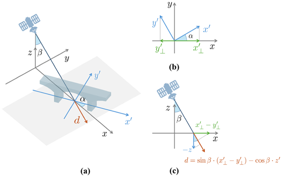
Satellite reference system
The LOS displacement of PS
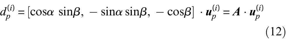
where

InSAR phase model with structural constraints
Replacing the LOS displacement term in the PSI phase model (Equation (4)) returns:
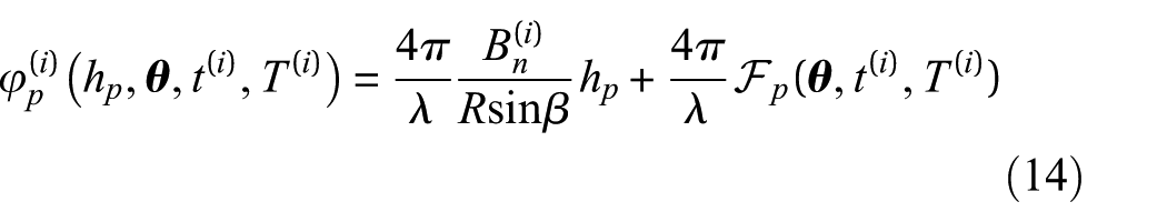
To estimate the unknown parameters
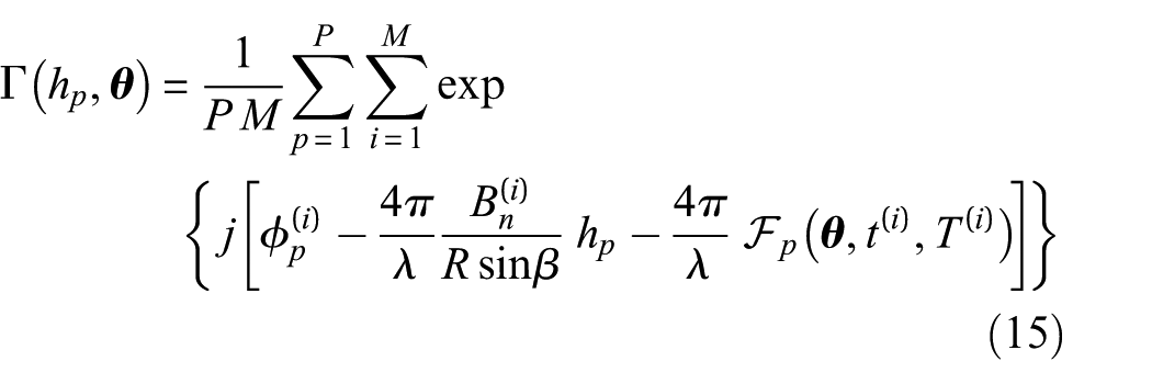
where
Several efficient global optimisation algorithms have been presented in the scientific literature, 36 and most widely used scientific programming environments offer reliable implementations of these methods. In this work, the particle swarm optimization (PSO) technique37–39 is used to solve the optimisation problem. Additional information is provided in the fourth section.
It should be noted that the precise location of PSs can be affected by uncertainty, as they could be located not only in the surroundings but also on structural elements other than those modelled. 40 However, the consistency between the structural model and the actual PSs spatial distribution can be verified by recomputing the temporal coherence – substituting the modelled phase of Equation (14) into Equation (9). PSs whose displacement phase time series is not consistent with the assumed deformation model will produce low temporal coherence and can be filtered out of the processing data. If a further consistency check is required, PSs with an estimated height falling outside the expected deck elevation (within a tolerance given by the scatterer height sensitivity) can be excluded.
Case study
Colle Isarco Viaduct
The case study selected for the application of the framework is the Colle Isarco Viaduct in Vipiteno, Italy. This structure was constructed in 1968 and opened later in 1971 and is now part of the A22 Highway. It has a total length of 1028 m, consisting of two parallel and independent decks and 13 spans.
The portion of major interest is the main spans between piers 7–8 and 9–10, consisting of symmetrical prestressed concrete Niagara box girders, with a filler beam (Gerber beam) connecting them. Each of the two elements is divided into a main span of length 91 m and a cantilever span of 59 m. Supported by the two cantilevers, there is a suspended beam of length 45 m. The box girders have a height 10.93 m on top of piers 8 and 9, and decrease to 2.57 m at the half-joints. Technical drawings of the plan and section views are reported in Figure 7.
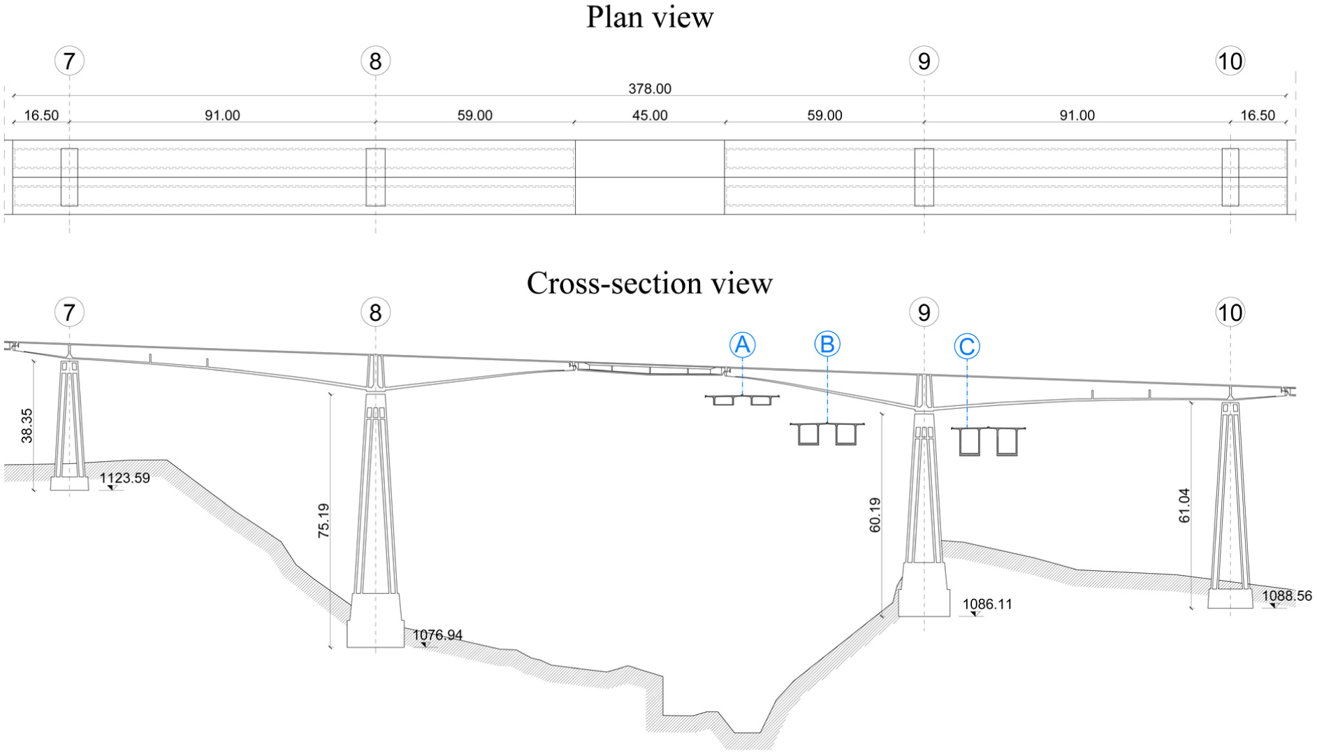
Plan and side views of the viaduct portion between piers 7 and 10.
The viaduct underwent progressive deflection over time, which led to major retrofitting interventions, first in 1988 and then in 2014. Since the 2014 intervention, the spans between piers 7 and 10 have been instrumented with 72 optical prisms, 50 of which are on the deck (see Figure 9(a) and (b)), for displacement monitoring. Additionally, fibre-optic sensors and thermocouples were installed on both the top and bottom slabs at the midspan, pier 8, and the cantilever half-joint, to measure deck deformations and local temperature, respectively. For these sections, it is therefore possible to estimate the temperature gradient, computed as the difference between the temperature recorded in the upper slab and the one measured in the bottom slab.
PSI analysis of the viaduct
A PSI analysis of the viaduct was carried out by Tonelli et al. 13 using a dataset of 62 COSMO-SkyMed X-band images acquired in stripmap HIMAGE mode, in descending orbit, between 5 July 2016 and 25 June 2020, with reference image corresponding to 18 March 2018 (shown in the star-graph of Figure 8(a)). The analysis resulted in the identification of 173 PSs on piers 7–10 segment.
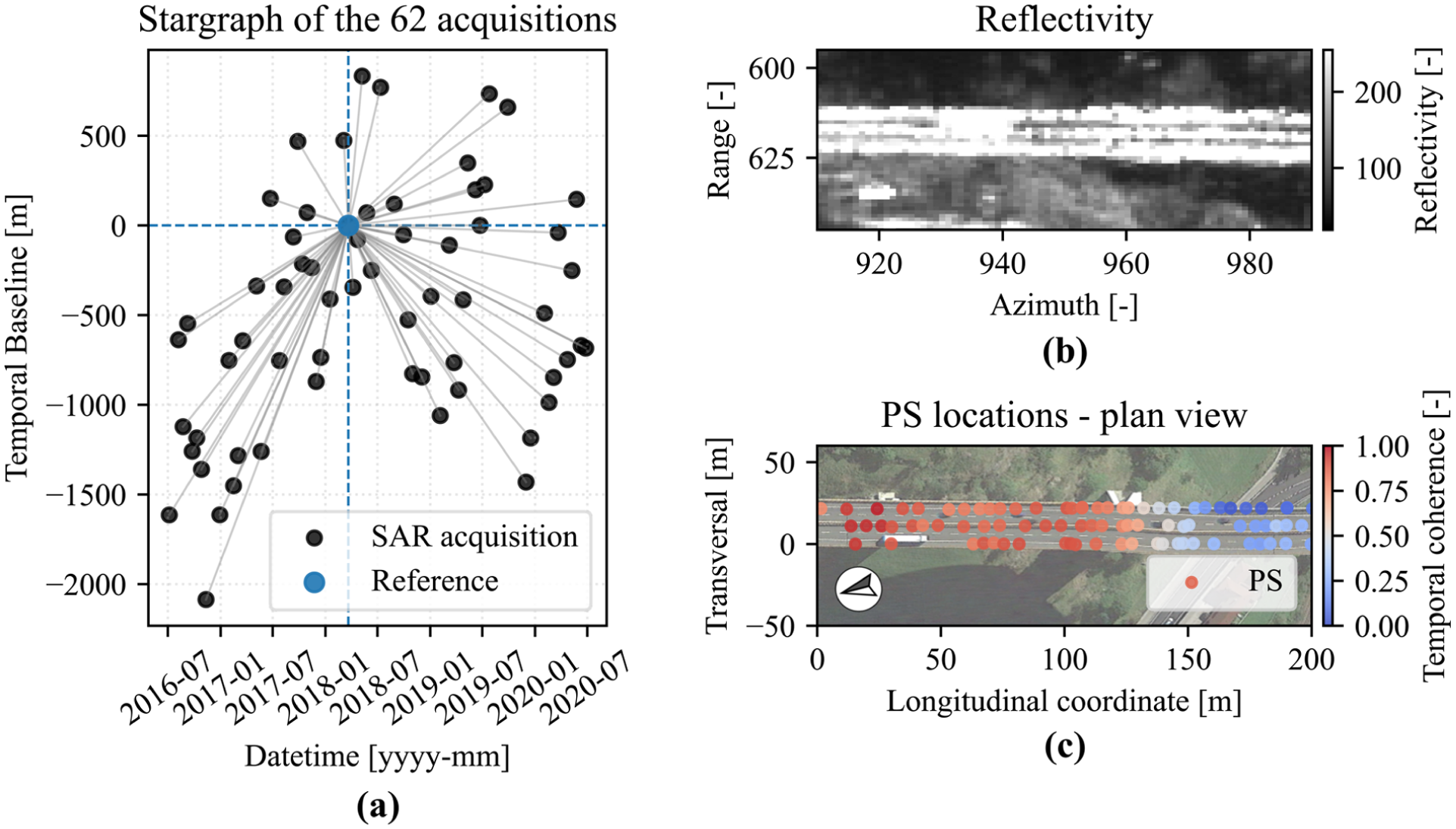
(a) Star graph showing temporal and perpendicular baselines of the 62 SAR images, (b) reflectivity map and (c) PSs distribution coloured by temporal coherence. SAR: synthetic aperture radar.
As shown in the plan distribution in Figures 8 and 9, the PSs align along three longitudinal lines, corresponding to the backscatter from the guardrails. The central line contains the reflection from both carriageways, which fall within the same SAR resolution cell. This phenomenon is visible in the reflectivity map of the piers 7–8 segment in Figure 8(b). Both figures also report the temporal coherence
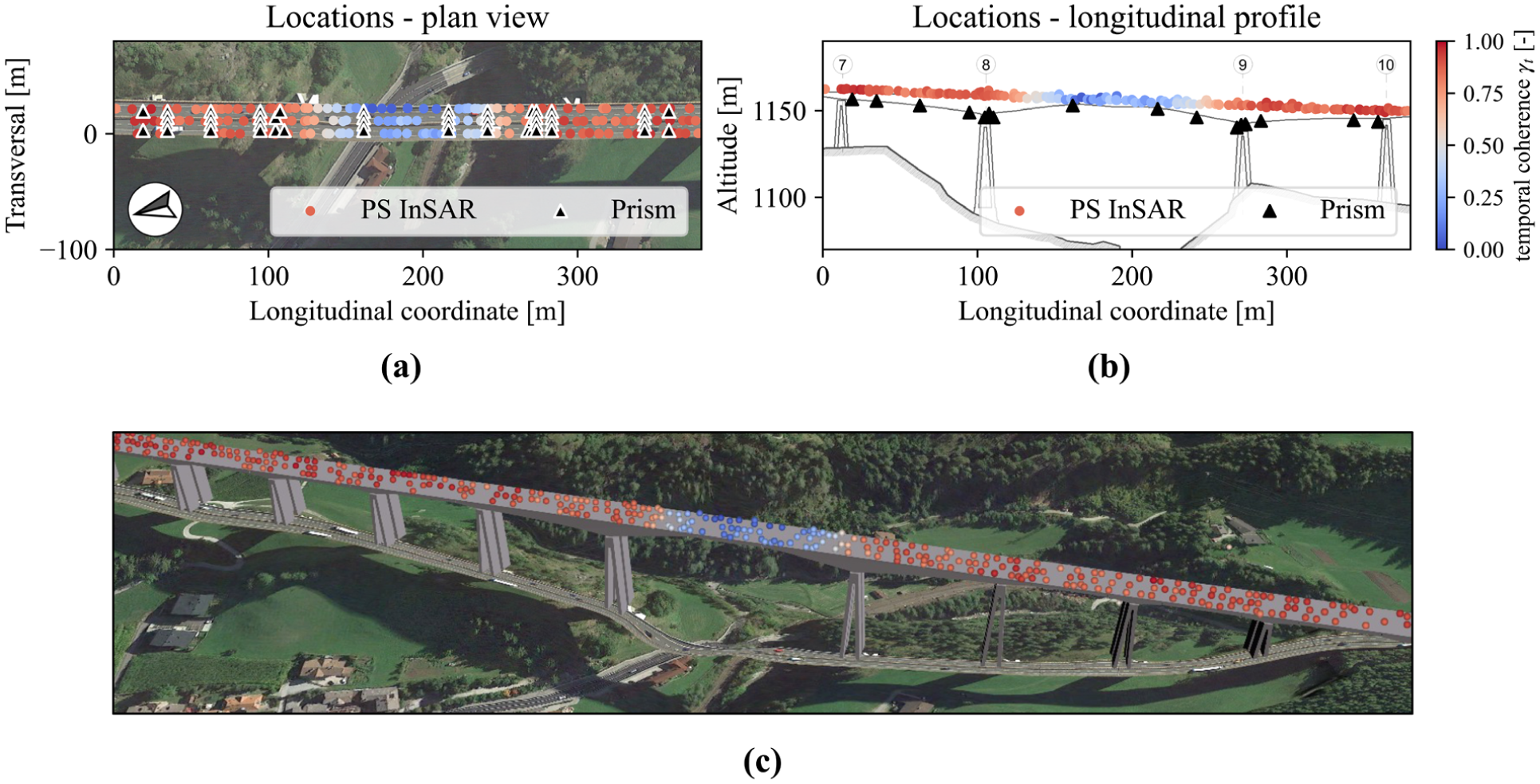
PSs distribution coloured by temporal coherence
In both figures, a significant reduction in temporal coherence can be observed near the ends of the cantilevers, in the vicinity of the half-joints, and on the Gerber beam, with values as low as 0.08. Temporal coherence progressively increases towards the piers and the main span, where overall high values are observed – particularly at the piers, with coherence values reaching up to 0.90.
To understand this phenomenon, it is useful to recall the two fundamental assumptions of PSI monitoring (explained in the second section): (
In order to verify whether these assumptions are satisfied for the actual structural behaviour, topographic measurements (i.e. true displacements) were projected on the satellite LOS. The displacement time series, relative to the reference acquisition, are reported in Figure 10, and their Pearson’s correlation indexes with air temperature and temperature gradient at selected locations. In the figure, four representative points on the north carriageway are considered: at pier 7 (blue), at the middle of the main span (orange), at pier 8 (green) and at the half-joint (red).
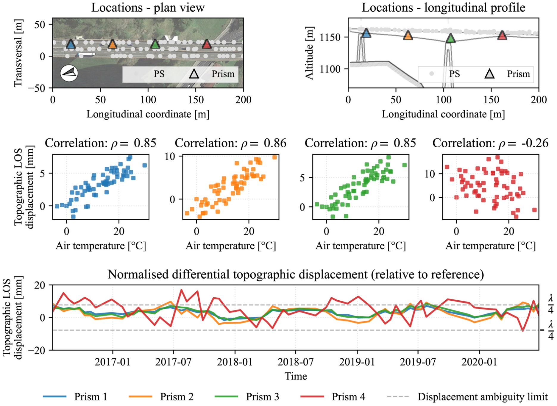
LOS-projected topographic displacements at four locations, their correlation with air temperature, temperature gradient across the section, and corresponding displacement time series. LOS: line of sight.
At the piers and at the midspan, LOS displacements are relatively contained within the ambiguity bounds and have strong correlation with air temperature
When considering correlation with the deck temperature gradient, a different behaviour is observed. All points exhibit a significant correlation with the temperature gradient; however, the relative importance of this parameter varies spatially. At piers 7 and 8, the correlation with temperature gradient is weaker (
For brevity, results for the southern carriageway are not reported, but they exhibit the same behaviour.
In summary, PSI analysis is expected to perform well for some of the viaduct points, whereas it is expected to fail on the cantilever span where the fundamental assumptions are violated, as will be confirmed by the experimental results presented in the fifth section. In this region, displacements are dominated by temperature gradient, not represented in the conventional PSI displacement model.
ST-InSAR analysis
To overcome the limitations discussed in the previous sections, the proposed ST-InSAR framework is applied following the methodology explained in the third section. The principal task is to define a structural model of the viaduct that describes its expected spatio-temporal deformation behaviour, therefore enabling the spatial correlation among PSs located on the deck. The parameters of this structural model are then jointly estimated within the interferometric analysis, and the correct LOS displacements are subsequently evaluated.
Dataset
The same dataset used for the PSI analysis was employed, consisting of
To ensure a fair comparison between ST-InSAR and PSI, only the PSs previously identified on the piers 7–10 segment by the previous PSI analysis were processed. A total of
Structural model
In order to apply the ST-InSAR framework to the interferometric phase time series, it is first necessary to define an appropriate structural model of the viaduct case study. The structural analysis focuses on the main span and cantilever span supported by piers P7 and P8. This segment behaves as an isolated structural system, independent from the rest of the viaduct. Since SAR acquisitions primarily illuminate the bridge deck, the structural model is defined for the deck itself. Given the spatial distribution of the persistent scatterers, it is reasonable to assume that the structure behaves predominantly as a linear (1D) system that develops along its longitudinal axis.
InSAR measures the displacement along the satellite LOS, which represents a projection of the actual 3D displacement field, composed of longitudinal, transversal and vertical components. For the Colle Isarco Viaduct, the satellite descending orbit creates a very small angle with the longitudinal axis of the bridge, which is approximately

(a) Footprint reference SAR image, (b) zoomed-in view of the viaduct P7–P10 with satellite azimuth direction and (c) projection of vertical displacement along the LOS. SAR: synthetic aperture radar; LOS: line of sight.
The vertical deflection of the viaduct at acquisition
Deck displacement is also influenced by the expansion of the supporting piers. In contrast to the deck behaviour, the piers displacement is well correlated with time and air temperature. Pier motion is modelled as the superposition of a linear temporal trend and a uniform thermal expansion component, consistent with the conventional PSI displacement model (Equation (5)). Therefore, for each carriageway, the displacement parameters include one linear displacement rate
To summarise, the proposed model for the Colle Isarco Viaduct relies on the following assumptions:
Each carriageway is modelled as a 1D Euler–Bernoulli beam with cubic shape functions. The model computes the displacement response at the deck edges, where the PSs are located.
Due to acquisition geometry and bridge type, the LOS displacement is assumed to depend only on the vertical displacement component.
Vertical deck deflection is driven by the temperature gradient between the upper and lower deck slabs. The gradient is treated as a separate parameter for each acquisition and, at a given time, is assumed spatially constant over the deck.
Pier displacements are treated as imposed boundary conditions and are modelled using a linear relationship with respect to time and air temperature.
The scheme of the model employed is illustrated in Figure 12.
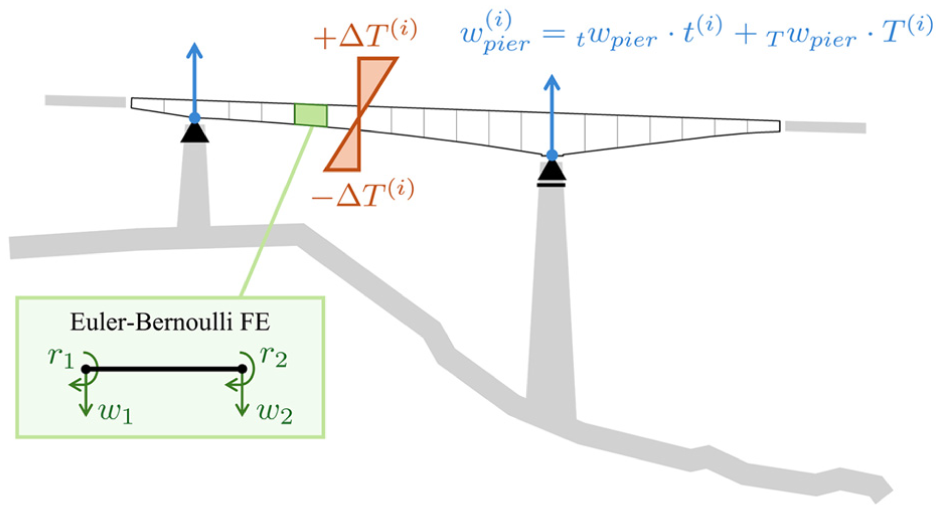
1D Euler–Bernoulli model employed for each carriageway of the segment P7–P8.
The resulting SP vector for each carriageway is therefore:
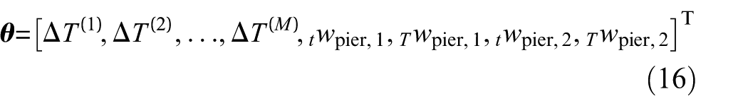
where
Regarding the number of PSs, a total of
Parameters identification
To find the optimal estimates of the parameters
Experimental comparison methodology
The LOS displacements measured using ST-InSAR are compared against both the conventional PSI displacement time series, and the topographic prism measurements used as validation benchmark. The performance of ST-InSAR is evaluated using the following metrics:
Root mean square of the error (RMSE) between SAR and topographic displacements time series, computed after removing of the mean value to eliminate bias;
Pearson’s correlation coefficient (
Updated temporal coherence (
Finally, the estimated temperature gradients
It is important to note that even the benchmark data are affected by uncertainty, which is due to:
Lack of temporal synchronisation, as topographic measurements timestamps do not coincide with SAR acquisitions, requiring interpolation;
Spatial misalignment, as PSs and prisms do not coincide exactly, so each PS is compared to its closest optical prism.
Consequently, the error observed in the performance evaluation reflects the combined effect of InSAR measurement errors and the spatial and temporal misalignment relative to the validation benchmark.
Results
This section presents the results obtained from the proposed ST-InSAR analysis. The performance of ST-InSAR is assessed through a comparison with that of PSI. Furthermore, both methods are validated against independent topographic benchmark measurements.
The comparison is carried out both graphically, through Figures 13 to 15, and numerically using the metrics reported in Table 1. The results corresponding to eight different points are reported, selected as the closest available persistent scatterers to the monitored topographic prisms on the viaduct deck. In addition, temporal coherence obtained by both PSI and ST-InSAR is analysed for all the extracted PSs along the structure. Finally, temperature gradients estimated by ST-InSAR are compared with independent measurements collected from thermocouples embedded in the viaduct deck.
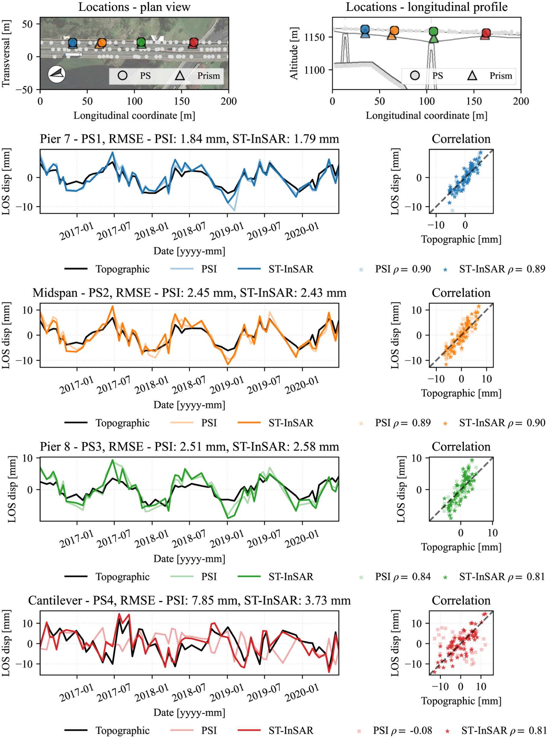
North carriageway, PS 1 (pier 7), PS 2 (midspan), PS 3 (pier 8), PS 4 (cantilever) – ST-InSAR results, compared with PSI and topographic measurements. ST-InSAR: spatio-temporal InSAR; PSI: persistent scatterer interferometry.
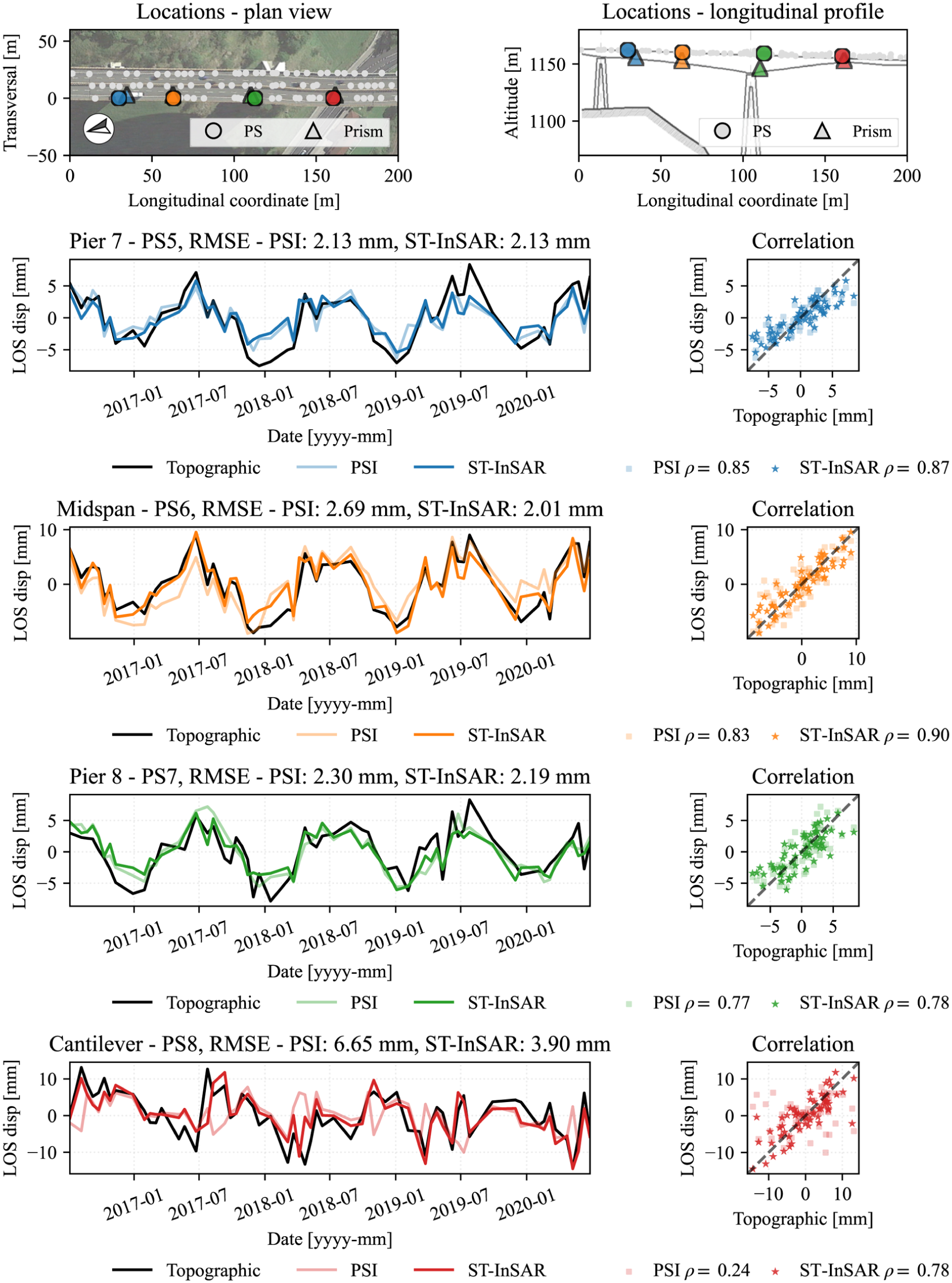
South carriageway, PS 5 (pier 7), PS 6 (midspan), PS 7 (pier 8), PS 8 (cantilever) – ST-InSAR results, compared with PSI and topographic measurements. ST-InSAR: spatio-temporal InSAR; PSI: persistent scatterer interferometry.
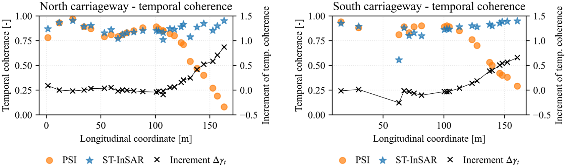
Temporal coherence of PSI and of ST-InSAR along the viaduct. ST-InSAR: spatio-temporal InSAR; PSI: persistent scatterer interferometry.
Performance comparison of ST-InSAR and PSI.
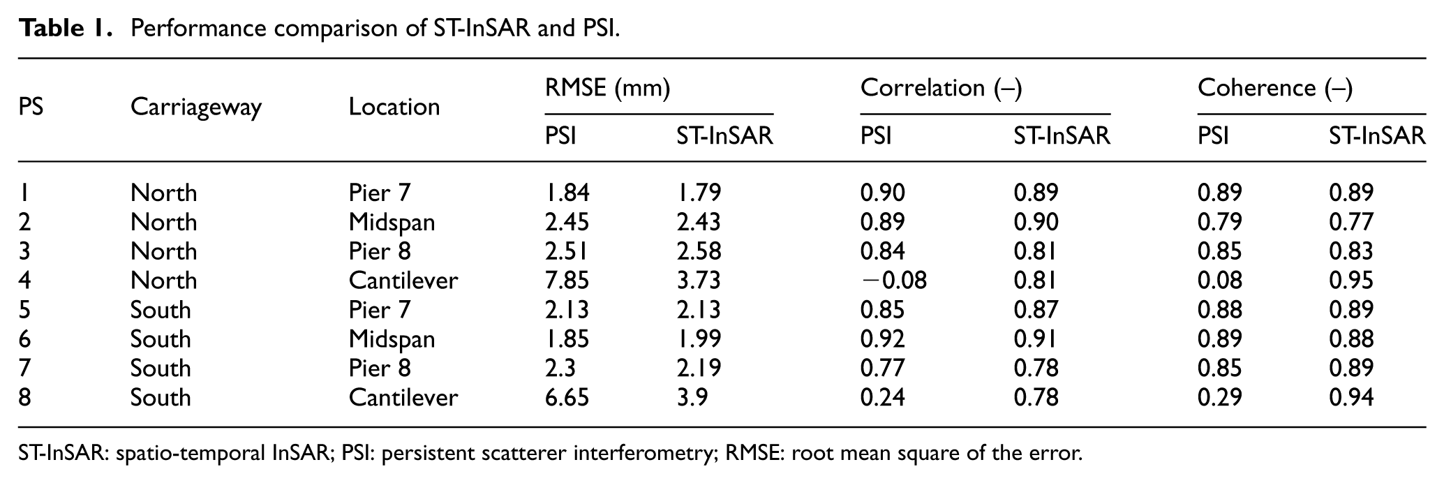
ST-InSAR: spatio-temporal InSAR; PSI: persistent scatterer interferometry; RMSE: root mean square of the error.
Comparison of ST-InSAR and PSI with benchmark measurements
The analysis first focuses on the northern carriageway. Figure 13 illustrates the comparison between the performance of ST-InSAR and PSI, both validated against the benchmark topographic measurements. At the top of the figure, the locations of the analysed PSs, together with the corresponding optical prisms used for topographic measurements, are shown in the plan and longitudinal profile. The lower panels report the LOS displacement time series (left) and correlation plots (right), where topographic measurements are shown in black, ST-InSAR results are indicated by bold lines, and PSI results by lightly transparent lines. The points reported are PS 1 close to pier 7 (blue), PS 2 at the midspan (orange), PS 3 at pier 8 (green) and PS 4 at the cantilever half-joint (red).
It can be immediately observed that ST-InSAR and PSI show very similar performance for PS 1, 2 and 3. Qualitatively, the LOS displacement time series estimated by the two techniques match well, although small discrepancies with respect to the topographic measurements are visible. This behaviour is expected, as discussed previously, since the benchmark measurements are affected by uncertainty due to temporal resampling and spatial misalignment relative to the SAR acquisitions. Figure 13 also show the correlation between InSAR-derived displacements and the topographic measurements (right). Again, for PS 1, 2 and 3, the distributions obtained using ST-InSAR and PSI largely overlap and strongly align along the principal correlation direction.
These observations are supported by the quantitative metrics reported in Table 1. For PS 1, 2 and 3, correlation coefficients of both methods are very similar, with overall satisfactory values greater than 0.8, meaning that PSI and ST-InSAR produce very similar displacements. Temporal coherence shows a similar trend: PSs located at the piers and midspan exhibit high PSI coherence (0.79–0.89), and similar values are obtained with ST-InSAR (0.77–0.89). In terms of accuracy, for the same locations, the two techniques substantially produce comparable results with an error on the order of around 2 mm. More specifically, RMSE values range between 1.84 and2.51 mm for PSI and 1.79–2.51 mm for ST-InSAR.
A marked difference in behaviour is observed for PS 4, located at the cantilever half-joint. At this location, PSI fails to correctly estimate the displacement time series, whereas ST-InSAR shows satisfactory agreement with the topographic measurements. The better performance of ST-InSAR is visible in both the displacement time series and the correlation plot (Figure 13 bottom panels). This is also evident by the correlation indexes in Table 1. For PS 4, PSI correlation coefficient drops to −0.08, together with a very low temporal coherence of 0.08, indicating poor modelling of the observed interferometric phase. Conversely, ST-InSAR achieves a correlation coefficient of 0.81 and a temporal coherence of 0.95 at the same point. RMSE is significantly lower for ST-InSAR 3.73 mm compared to that of PSI 7.85 mm, particularly considering that the true signal amplitude at this point is on the order of 10 mm.
Very similar insights can be drawn for the southern carriageway, based on the displacement time series and correlation plots shown in Figure 14, and the performance metrics reported in Table 1.
Analysis of temporal coherence
It is reminded that temporal coherence quantifies the similarity between the observed and the modelled interferometric phase and therefore does not depend on the availability of benchmark measurements. Consequently, temporal coherence can be evaluated for all persistent scatterers on the viaduct.
Figure 15 shows the temporal coherence values obtained with PSI (orange) and ST-InSAR (blue) for the various PSs along the deck, on both carriageways, together with the corresponding increases (black) brought by the proposed method with respect to PSI.
The figure shows a spatial trend for PSI, where coherence is highest near the piers (at longitudinal coordinates of approximately 16.5 and 105 m) and remain overall high in the main span (greater than 0.75), while it progressively decreases towards the cantilever half-joints.
ST-InSAR coherence exceeds the 0.75 threshold for nearly all points on the structure, with one exception on the south carriageway where coherence decreases from 0.81 (PSI) to 0.55 (ST-InSAR).
Temperature gradient estimation
The deck temperature gradient, estimated by ST-InSAR as one of the model parameters, is compared to the measurements acquired by the installed thermocouples – embedded in the deck concrete beams. Figure 16 shows the measured temperature gradient
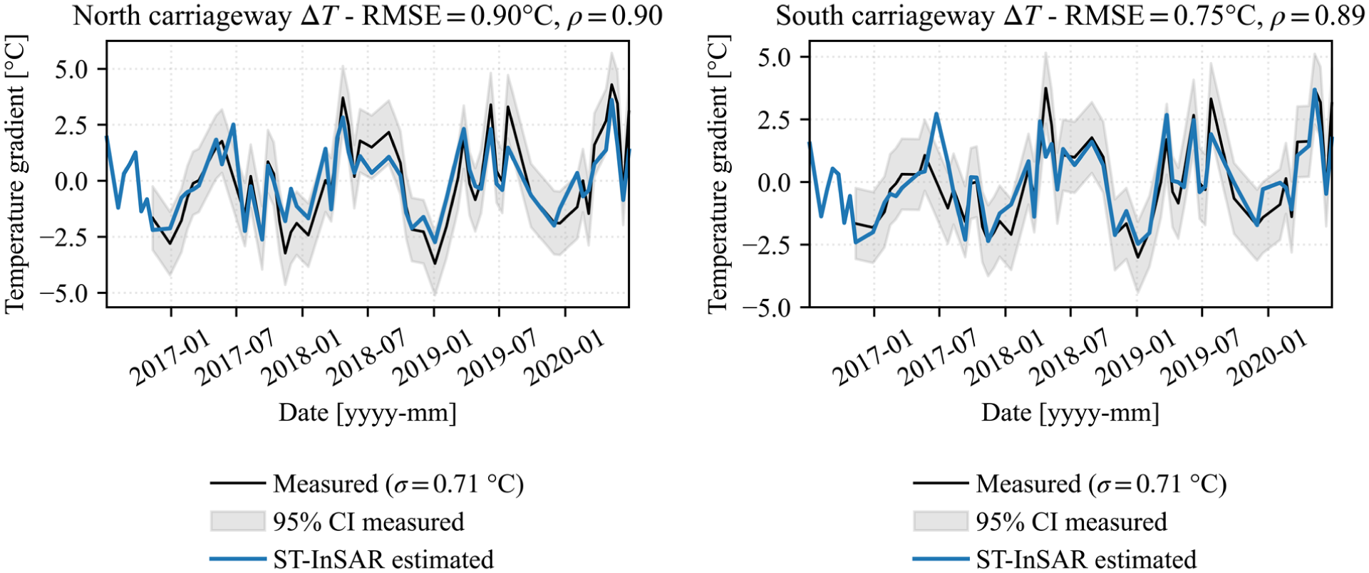
Extracted temperature gradient time series compared to average gradient measured.
A strong agreement between the measured and estimated temperature gradients can be observed. In particular, the correlation coefficients between the thermocouple measurements and ST-InSAR estimates are 0.90 and the values measured by the monitoring system – is below 1°C for both carriageways, with values of 0.90 and 0.75°C for the northern and southern carriageway, respectively.
Discussion
Why PSI fails at specific locations
The results presented in the fifth section highlight a clear spatial dependence of PSI performance along the Colle Isarco Viaduct. The technique is effective at piers and at the midspan, while its performance degrades along the cantilever spans.
To interpret this behaviour, it is recalled that conventional PSI assumes that the displacement is a linear function of time and air temperature, and that it remains within the ambiguity limit
Based on the ground monitoring system installed on the Colle Isarco Viaduct, it is expected that PSI performs well in structural regions where these assumptions are valid and degrades where they are violated. The true LOS displacement analysis presented in the fourth section – through Figure 10– supports this expectation:
At the piers, structural displacements are primarily dominated by uniform thermal expansion and, therefore, show strong correlation with air temperature. Consequently, the PSI displacement model (Equation (5)) remains representative of the observed interferometric phase, resulting in high temporal coherence.
High temporal coherence is also obtained at the midspan, where the air-temperature correlation is less but still significant
Moving away from pier 8 towards the cantilever half-joints, the structural response becomes increasingly dominated by temperature gradients, which induce vertical thermal deflection of the deck. Since this deformation mechanism is not explicitly represented in the conventional PSI model, this results in a gradual loss of PSI performance. This is supported by spatial trend observed in the coherence maps, and by the RMSE error estimated at the half-joints.
Why ST-InSAR performs well where PSI fails
Unlike PSI, the proposed ST-InSAR framework employs a structural deformation model that explicitly accounts for both the uniform thermal expansion of the piers and the effects of temperature gradients across the deck.
Effectively, this model captures more accurately the correct deformation mechanisms, making ST-InSAR more effective in regions where PSI particularly struggles, such as the cantilever spans. At these locations, evidence demonstrates that ST-InSAR provides displacement estimates that better describe the true structural response. The improved deformation modelling naturally leads to a more accurate approximation of the interferometric phase, which in turn results in higher temporal coherence.
In regions where the assumptions of conventional PSI are satisfied, ST-InSAR performs comparably to PSI. However, it significantly outperforms PSI at the cantilever spans, producing better RMSE and correlation values associated with the displacement time series.
The key difference of the proposed approach is that it consists of simultaneously processing all the persistent scatterers located on the structure while defining spatial correlation compatible with the structural model. This constraint effectively limits the solution space only to physically feasible deformation configurations – compatible with the expected structural behaviour.
Metrological accuracy of ST-InSAR
Overall, ST-InSAR achieves an accuracy comparable across all stable reflective points on the bridge were validated against benchmark measurements. LOS displacement uncertainties (RMSE) are consistently of the order of 2 mm at the piers and midspan, while slightly higher, of the order of 3 mm, at the cantilever half-joints. This happens because the error is combination of, on the one side, the metrological uncertainty of InSAR measurements and, on the other, the temporal and spatial misalignment of the topographic benchmark (as described in ‘Experimental comparison methodology’ section).
It is reasonable to assume that the metrological uncertainty of InSAR does not depend on the displacement amplitude, while the error associated with the benchmark misalignment does. Therefore, at points where displacement amplitudes are relatively small, the resulting RMSE is expected to be primarily governed by the measurement uncertainty of InSAR. On the contrary, at points undergoing larger displacements, the misalignment error becomes increasingly more significant.
More specifically, for pier 7, pier 8 and the midspan – where displacement amplitudes are limited – the RMSE is very similar, around 2 mm (between 1.79 and 2.58 mm). Here, PSI returns comparable errors. This suggests that the metrological uncertainty of InSAR is approximately 2 mm.
Conversely, as expected, the RMSE of ST-InSAR increases to about 3 mm at the half-joints, where larger displacements occur. It must be noted that this increase does not reflect a degradation of ST-InSAR accuracy but rather results from the increasing contribution of benchmark misalignment. Overall, the InSAR metrological uncertainty is therefore expected to remain constant across the structure and approximately 2 mm.
At the same locations, on the contrary, the RMSE associated with PSI is comparable to the true displacements magnitude.
It is worth noting that an uncertainty of 2 mm is comparable to the order of magnitude of the error typically associated with topographic surveying techniques. A key difference, however, is that topographic measurements are not collected synchronously, as total stations acquire sequentially at individual points, whereas InSAR measurements are acquired simultaneously over the entire structure. Therefore, ST-InSAR could have potential also for reconstructing the instantaneous deformed shape of the structure.
Using ST-InSAR to identify the thermal field
ST-InSAR employs a displacement model that depends on both air temperature and the temperature gradient across the bridge deck. While air temperature is treated as a known input, as in conventional PSI, temperature gradient is not directly measured and is assumed as an unknown parameter to be estimated from the analysis.
The results presented in ‘Temperature gradient estimation’ section, demonstrate that the temperature gradient estimated through ST-InSAR is actually very close to the true gradient, with an error smaller than
Notice that, in opposition, gaining information from PSI about the temperature field of the structure is not possible.
Drawbacks of using ST-InSAR
Based on the discussion above, ST-InSAR proves to be more effective than conventional PSI approach. In spite of that, its application also introduces drawbacks compared to PSI.
Firstly, ST-InSAR requires the definition of a physics-based structural model that accounts for deformation mechanisms influencing the structure. If deformation sources are not represented in the model, their displacement contribution cannot be estimated. Therefore, the structural model must be sufficiently comprehensive to describe all the physical phenomena governing the structural response. This limitation, however, does not constitute an additional requirement with respect to conventional contact-based SHM. In this context, structural geometry, construction details, and expected deformation mechanism are also needed to design sensor layouts and interpret measurements.
Second, applying the framework to a bridge or viaduct requires a preliminary investigation to define the geometry, orientation – as well as the appropriate modelling assumptions – for the structure of interest. It is also necessary to precisely identify the main structural components with their corresponding scattering elements in the SAR reflectivity map. For instance, when piers are particularly tall, radar shadowing can assist in identifying their positions. Alternatively, corner reflectors may be installed to enhance the backscattering of selected locations and ensure accurate correspondence between structural nodes and persistent scatterers. It is noteworthy that the applicability of ST-InSAR is constrained by the need for a physics-based representation of deformation mechanisms, geometry and structural orientation, thereby limiting the intrinsic benefits of synthetic radar interferometry in terms of cost-effectiveness, deployment efficiency and large-scale scalability.
As mentioned in the third section, the spatial uncertainty in PS distribution can be addressed by examining the recomputed temporal coherence. In the present case study, this issue is further mitigated by the fact that only PSs previously identified on the deck by the preceding PSI analysis were processed, ensuring that both methods operated on the same set of scatterers. The high temporal coherence values obtained further confirm that the identified PSs are consistent with the modelled deck deformation, supporting their correct structural assignment. However, this issue may become more challenging when merging data from multiple orbits or sensors, where differences in viewing geometry and resolution may require more explicit classification strategies such as that proposed by Giordano et al. 40
A further consideration concerns the robustness of the estimation when the number of unknown parameters in Equation (16) is large. As the structural complexity increases, the number of SPs
Finally, although this work focuses on bridges and viaducts, the same methodology can be extended to other civil structures – such as dams, buildings, port facilities and towers – provided that their displacement behaviour can be spatially correlated by an appropriate physical model.
Conclusions
This work presented a spatio-temporal framework that integrates physics-based structural models into the MT-InSAR processing pipeline. The proposed method exploits the structural model to simultaneously estimate displacement information from all persistent scatterers identified on the structure, explicitly accounting for spatial and temporal correlation.
The methodology was applied to the Colle Isarco Viaduct as a case study, where the performance of the proposed ST-InSAR was compared with that of conventional multi-temporal PSI, by using benchmark topographic measurements.
Based on the results, the following conclusions can be drawn:
Conventional PSI presents several limitations when applied to bridges and viaducts. This technique performs well when displacements are limited and correlated with air temperature. Consequently, it fails when displacements and not well correlated with air temperature and exceed
ST-InSAR performs well at all monitored locations, successfully identifying displacements at points where conventional PSI fails – where deformation is not correlated with air temperature and exceeds the ambiguity limit. This is achieved thanks to the integration of a more refined displacement model that accounts for deformation mechanisms typically neglected in conventional PSI and jointly estimating the displacements across all persistent scatterers. As a result, temporal coherence at locations poorly identified by PSI increases significantly, from values close to zero (0.08) to highly satisfactory levels (up to 0.95).
The comparison with the benchmark measurements suggests that the metrological error of ST-InSAR is on the order of 2 mm, which is on the same order of magnitude achieved by topographic surveying monitoring. A significant advantage of ST-InSAR, however, is the capability of synchronously measuring all points on the structure. Under appropriate conditions, this makes ST-InSAR a promising solution alternative to topographic survey monitoring.
A by-product of ST-InSAR is the identification of the thermal gradient across the bridge deck. In this study, the deck temperature gradient was estimated with an accuracy below 1°C. Therefore, ST-InSAR could also be used to infer the thermal field of the structure, in addition to displacement monitoring.
The proposed methodology can be extended to civil structures beyond bridges, provided that their displacement behaviour can be described through an appropriate physics-based spatial correlation model.
The main limitation of ST-InSAR lies in the requirement of a physics-based structural model that captures the relevant deformation mechanisms, geometry and orientation of the structure. This prerequisite may compromise key advantages of SAR interferometry, such as low-cost, rapid monitoring and scalability across large infrastructure typologies. This limitation may be mitigated by automating model generation through approaches such as parametric modelling, digital twins and hybrid physics–data-driven methods.
Future work will focus on developing a Bayesian inference framework to enhance the robustness of the estimation, particularly in scenarios where multiple deformation mechanisms contribute to the structural response.
Footnotes
Acknowledgements
The authors would also like to thank A22 Autostrada del Brennero, in particular David Quattrociocchi and Carlo Costa, for sharing the topographic survey data. COSMO-SkyMed products have been provided free of charge for research purposes by the Italian Space Agency, Project Card ID: 630 “SAR SHM of bridges”.
Funding
The authors disclosed receipt of the following financial support for the research, authorship, and/or publication of this article: The study presented was funded by: the ReLUIS Interuniversity Consortium under the agreement DPC-ReLUIS 2020-2022 and DPC-ReLUIS 2024-2026 WP 6 ‘Monitoring and satellite data’ and the European Union – Next Generation EU, Mission 4 Component 2 – CUP E53D23003560006.
Declaration of conflicting interests
The authors declared no potential conflicts of interest with respect to the research, authorship, and/or publication of this article.