
Abstract
Structural health monitoring of mechanical assets can be hindered by environmental variability that causes distribution shifts between training and deployment. Many domain adaptation (DA) methods mitigate these shifts but behave as black boxes with limited insight into how representations change. This work introduces a novel interpretable framework, scattering-based prototype-aligned DA, that combines physics-guided feature extraction, synthetic data generation and prototype-based alignment for robust damage detection under temperature variation. A convolutional conditional variational autoencoder, trained on healthy data across temperatures with multi-domain reconstruction losses, generates temperature-conditioned synthetic damaged guided-wave signals from limited baseline damage measurements and healthy responses, creating a controlled testbed when damaged data at other temperatures are unavailable. Prototype-based domain adversarial training with gradient reversal and entropy-gated pseudo-labelling aligns source and target feature manifolds while preserving damage-sensitive patterns. Interpretability modules based on prototype trajectories, instance to prototype similarities and low-dimensional visualisations reveal how decision boundaries and latent representations evolve. Experiments on composite structures across temperatures show that the framework improves robustness over baselines and maintains high diagnostic accuracy while providing actionable insight into the adaptation process and enabling informed diagnostic assessment by domain experts in safety-critical contexts.
Keywords
Highlights
Interpretable domain adaptation improves damage detection under temperature change.
Physics-guided features reduce environmental influence while keeping damage patterns.
Synthetic temperature-conditioned signals enable training when damage data are scarce.
Prototype-based alignment explains how decisions shift across operating conditions.
Validated on composite plates and wind turbine blades across multiple temperatures.
Introduction
Structural health monitoring (SHM) of mechanical assets faces fundamental challenges when deploying damage detection models across data scarcity and varying operational conditions. 1 Temperature fluctuations, humidity variations, boundary condition changes and manufacturing tolerances introduce distributional shifts that severely degrade the performance of models trained in laboratory settings when applied to field conditions. 2 This domain shift problem is particularly acute in safety-critical applications such as wind turbine blades (WTBs), aerospace composites and civil infrastructure, where acquiring labelled damage data for each individual asset is economically prohibitive, while the consequences of missed detections can be catastrophic. 3 The core challenge lies not merely in achieving robust performance but in providing transparent evidence that damage-sensitive features are preserved during the transition from controlled environments to operational deployment. 4
Environmental and operational variabilities (EOVs) have motivated extensive research into robust feature extraction methods. Classical time and frequency domain descriptors, while computationally efficient, exhibit brittleness under temperature and operational variations. 5 Wavelet transform and its variants such as wavelet time scattering (WTS) have emerged as a promising physics-guided approach, providing deformation-stable representations through cascaded wavelet transforms and modulus operations without requiring learned parameters. 6 Ojha et al. 7 demonstrated improved robustness compared with conventional scalogram features in composite impact localisation, while Rezazadeh et al. 8 showed effective extraction of damage-sensitive features under operational variations in rotor systems using WTS combined with long short-term memory networks. Ma et al. 9 coupled scattering transform features with least squares proximal twin support vector machines, demonstrating robust fault diagnosis under noise in rotating machinery. However, these applications treat WTS merely as preprocessing without exploiting its invariance properties to facilitate domain adaptation (DA). Critically, existing work does not leverage the well-characterised stability properties of WTS to provide robust features that support knowledge transfer between operational conditions.
The challenge of transferring knowledge between different operational regimes has driven the development of DA techniques for SHM. Bull et al.10,11 established population-based SHM concepts for knowledge sharing across similar assets through statistical mixture models. Wang et al. 12 employed adversarial DA between finite element simulation and experimental data for fatigue crack detection, while da Silva et al. 13 used transfer component analysis to stabilise impedance-based diagnostics under temperature changes. Yang et al. 14 introduced multi-source dynamic adaptive generalisation for composite crack detection without requiring target domain labels. These methods achieve domain alignment through statistical criteria but most provide limited transparency regarding which signal characteristics are being aligned or whether physically meaningful patterns are preserved during adaptation. More recent efforts have begun to incorporate physical knowledge into the adaptation process, for instance by embedding physics-informed constraints within generative adversarial domain alignment for SHM, 15 while contrastive learning strategies have been integrated with adversarial DA to improve class-level feature discriminability during cross-domain fault diagnosis. 16 Notwithstanding these advances, existing approaches rarely offer systematic tools for tracking how class-level representations reorganise throughout the adaptation process or for verifying that damage-sensitive structure is maintained after domain alignment.
Environmental compensation strategies have evolved from baseline subtraction towards reference-free approaches that exploit physical invariants. 17 Salmanpour et al.18,19 developed comprehensive temperature correction procedures including minimum residual alignment, single baseline correction and instantaneous baseline mapping for guided wave monitoring, demonstrating effective compensation across thermal ranges. Amer and Kopsaftopoulos 20 embedded structural damage indices within Gaussian process regression to achieve baseline-free inference with probabilistic outputs. Yue et al. 21 proposed relative referencing that compares paths to each other rather than historical records, effectively reducing environmental drift at the feature level. While these compensation techniques successfully mitigate environmental effects, they operate on raw signals or hand-crafted features without leveraging the structured mathematical invariances that methods like WTS inherently provide, and function independently of DA mechanisms.
The deployment of machine learning models in safety-critical infrastructure has intensified the need for interpretable diagnostic systems. 22 Post hoc attribution techniques have been widely applied, with Kim and Kim 23 adapting Gradient-weighted Class Activation Mapping for vibration data, Yan et al. 24 employing SHapley Additive exPlanations to identify physics-guided features and Hanchate et al. 25 applying Local Interpretable Model-agnostic Explanations to highlight influential time-frequency regions. Ante-hoc interpretable architectures have received more limited attention, with Chen and Dong 26 proposing Sparse Temporal Logic Networks and Li et al. 27 introducing Variational Attention-based Transformers with sparse Dirichlet priors. However, these interpretability approaches focus exclusively on explaining predictions within single operational conditions, failing to address how representations transform during DA. Rezazadeh et al. 28 presented one of the few attempts to visualise internal changes during adaptation through activation pattern heat maps, although this post hoc visualisation does not guide the adaptation process itself. Prototype-based learning offers an interpretable alternative by representing each class through exemplar patterns corresponding to specific damage modes, 29 however its integration with DA for SHM remains largely unexplored.
The convergence of these research streams reveals critical gaps preventing confident deployment of domain-adaptive SHM systems. While WTS provides theoretically grounded invariances for environmental robustness, current applications do not exploit these properties to support DA, missing the opportunity to build adaptation upon physics-guided representations. DA techniques achieve statistical alignment without maintaining interpretable correspondence between source and target representations, leaving practitioners unable to verify that damage classes preserve their physical meaning. Environmental compensation and DA are treated separately rather than as jointly optimised processes. Most critically, no framework provides interpretable evidence of how damage-sensitive features transform during adaptation, preventing validation that transferred models retain physical validity rather than learning spurious correlations. These limitations raise fundamental research questions concerning how mathematical invariances of physics-guided feature extraction can be leveraged to facilitate interpretable DA in SHM. Furthermore, it remains unclear how damage-sensitive features preserve their physical meaning when transferred across operational conditions, and what mechanisms enable practitioners to verify that adaptation maintains structural rather than purely environmental patterns.
This work addresses these challenges through a novel unsupervised domain adaptation (UDA) framework (scattering-based prototype-aligned DA (SPADA)) integrating physics-guided feature extraction, prototype-based adaptation and dedicated diagnostic modules. The framework employs WTS as a principled front end, leveraging its mathematical stability to deformations and translation invariance to suppress certain EOVs while preserving damage-related modulations. The resulting scattering coefficients feed into a prototype-based UDA mechanism maintaining explicit correspondence between source and target exemplars. Separate interpretability modules, operating as post-training inspection tools without altering the optimisation dynamics, quantify prototype trajectories, instance-prototype similarity patterns, attention weight dynamics and low-dimensional separability, enabling practitioners to examine how the latent decision structure evolves during adaptation and to identify potential failure modes before deployment decisions are made.
The primary contributions are fourfold.
Demonstration of the mathematical invariances of WTS to provide stable, physics-guided features facilitating prototype-based UDA, ensuring feature representations are less sensitive to temperature while capturing damage-related modulations. This constitutes one of the first integrations of WTS-based feature extraction with interpretable transfer learning in SHM.
An interpretable prototype tracking mechanism that reveals how damage classes reorganise between temperature conditions while maintaining correspondence to physical damage modes, providing practitioners with evidence that adaptation preserves structural rather than purely environmental patterns.
An interpretability diagnostic method based on prototype trajectories, instance-prototype similarity matrices, attention weight evolution and low-dimensional visualisations that enable domain experts to assess whether changes remain consistent with known material behaviour under temperature variation.
The framework achieved classification accuracy comparable to black-box approaches while equipping practitioners with diagnostic tools to assess whether damage-sensitive patterns are preserved during adaptation, offering an interpretable alternative to opaque statistical alignment procedures.
The remainder of this paper is structured as follows. The second section presents the methodology, detailing the fundamentals of WTS and the proposed interpretable UDA framework. The third section describes the case studies, including the composite plate dataset and the WTB benchmark. The fourth section provides the results and discussion, examining the effects of EOVs on signal characteristics, feature extraction results, data augmentation outcomes, damage detection performance with and without DA and the internal activities of the proposed framework. The fifth section summarises the conclusions and outlines future research directions.
Methodology and methods
This section presents two complementary frameworks for temperature-dependent SHM under EOVs. First, a convolutional conditional variational autoencoder generates temperature-conditioned synthetic damaged signals from limited baseline damage and multi-temperature healthy data, addressing data scarcity. Second, the SPADA framework performs fault diagnosis under fully UDA, where target domain labels are unavailable. The integration of WTS, prototype-based attention and interpretability mechanisms enables robust cross-domain generalisation while maintaining diagnostic transparency.
Convolutional conditional variational autoencoder
A generative framework was developed to synthesise temperature-conditioned synthetic damaged guided-wave signals. This architecture integrates convolutional feature extraction with conditional variational inference to model the joint distribution of signals and temperature conditions. Latent-space offsets and amplitude masks produce synthetic signal variations reflecting temperature and structural damage influences inferred from the baseline condition, extending limited experimental datasets across operational environments.
Let
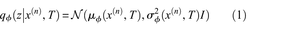
where

For damage level
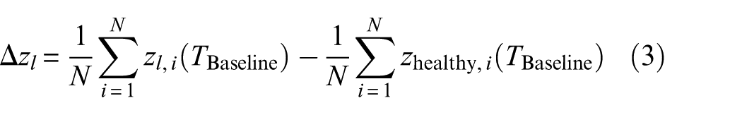
This offset characterises latent-space displacement from structural damage, serving as a transferable feature across temperatures. Per-channel and per-time amplitude masks are constructed from the analytic envelopes of the damaged and healthy signals at
A stochastic component is derived from the interquartile range (IQR) of the same ratios: the per-element dispersion is set as a fraction of the estimated standard deviation (approximated as IQR divided by 1.35), capped at a fixed proportion of the deterministic mask value to prevent extreme perturbations. During generation (Equation (5)), the decoded signal is first modulated by the deterministic mask via element-wise multiplication, and an additive Gaussian noise term
The training objective is a weighted composite of five terms:
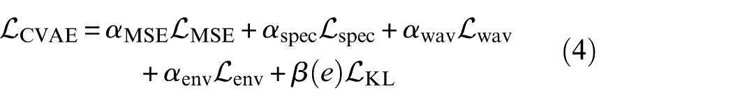
where
Final synthesised damaged signals at temperature
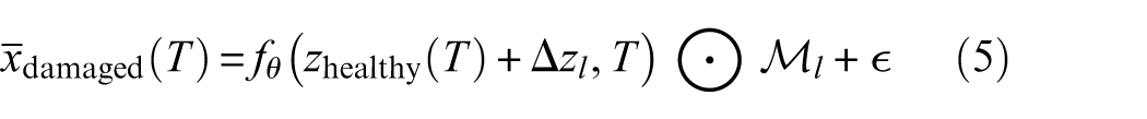
where
This method generates temperature-conditioned synthetic damaged signals using baseline damaged data at
A limitation of this synthesis strategy is that the latent offset
SPADA framework
SPADA addresses UDA where target labels are unavailable by integrating WTS for stable, translation-invariant feature extraction with prototype-based attention mechanisms that maintain class-level structure through source prototypes (using true labels) and target prototypes (employing entropy-gated pseudo-labels). Training combines four objectives: source classification via weighted cross-entropy with label smoothing, target pseudo-labelling on confident samples, adversarial domain discrimination through gradient reversal and prototype compactness encouraging source clustering. The pseudo-labelling mechanism with confidence gating and dynamic prototype updating distinguishes SPADA from purely adversarial approaches by actively generating and refining target labels while managing noise. Interpretability modules track prototype trajectories, similarity structure, attention dynamics and latent separation throughout training to diagnose adaptation quality and identify failure modes.
Wavelet time scattering
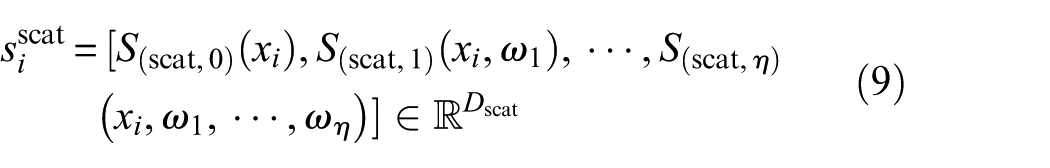
WTS processes signals through hierarchical operations: wavelet convolution for localised frequency content, modulus operation for stability enhancement, and averaging via scaling functions for translation invariance. For channel

where * denotes convolution and

where
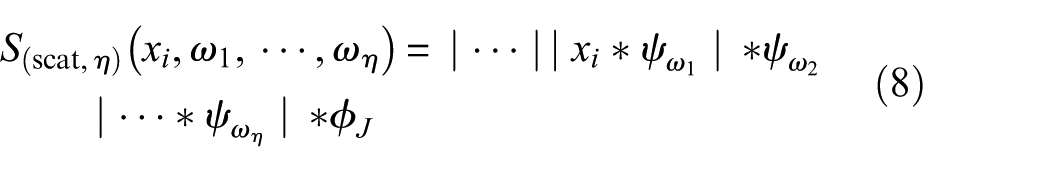
where
The scattering transform possesses formally established stability properties that underpin its suitability for cross-domain SHM. Mallat
31
proved that the scattering coefficients satisfy a Lipschitz continuity bound with respect to diffeomorphic deformations: for a signal

where
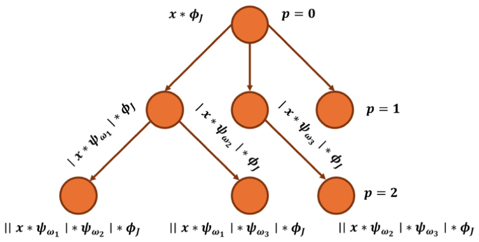
Schematic representation of the WTS process up to the second order for a single channel. WTS: wavelet time scattering.
Features are invariant to small temporal shifts, noise-robust and maintain discriminative properties essential for cross-domain fault diagnosis.
Domain adaptation
The DA block comprises four loss functions: source classification, target pseudo-label, domain adversarial and prototype alignment. A domain-adversarial neural network with shared feature extraction projects WTS features into shared latent space, calculating source classification and adversarial losses.
Prototype construction and attention-based updating
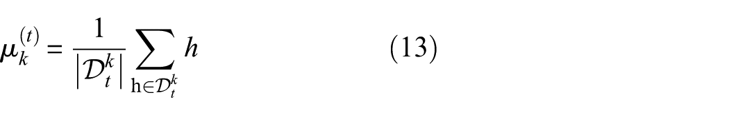
Class prototypes in latent space

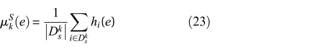
Source prototypes use true labels:
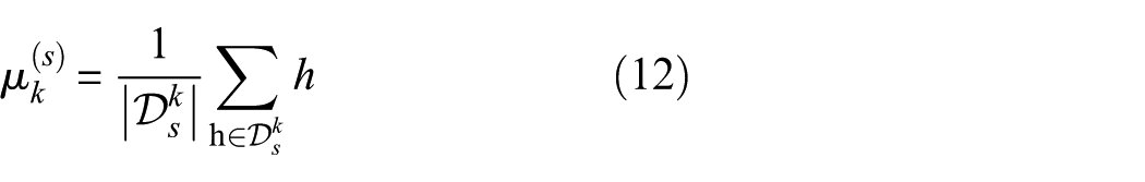
where
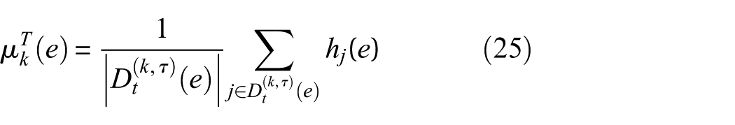
Target pseudo-labels derive from temperature-scaled softmax:
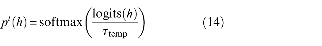
Temperature parameter
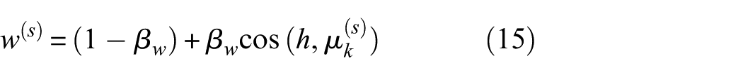
where
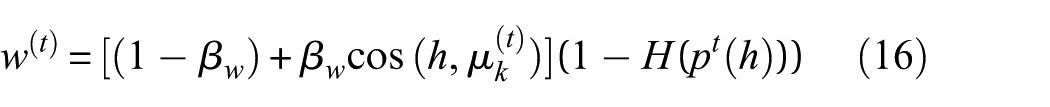
This mechanism ensures representative, confident samples contribute strongly. Prototypes are initialised at zero vectors in latent space. Since all features are standardised to zero mean and unit variance prior to training, zero initialisation places prototypes at the centroid of the standardised feature distribution rather than at an arbitrary location, providing a neutral starting point. Upon encountering the first mini-batch containing samples of class
Training objectives
The learning process employs four complementary losses.
(a) Source classification loss (
Weighted cross-entropy applies prototype-based attention weights to labelled source samples:
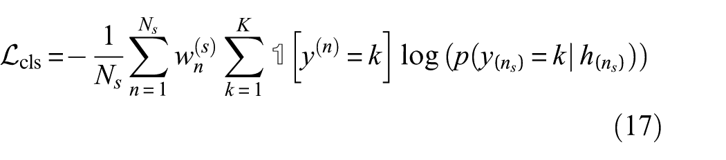
where
(b) Target pseudo-label loss (
This loss guides learning on unlabelled target data through confident pseudo-labels. Only samples passing confidence gate (
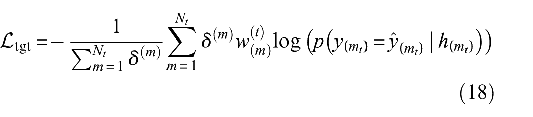
where
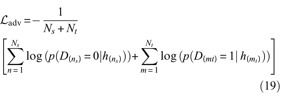
(c) Domain adversarial loss (
Domain discriminator distinguishes source and target while feature extractor prevents discrimination:
(d) Prototype alignment loss (
This enforces intra-class compactness within source domain:
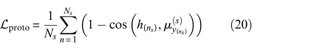
promoting class cohesion and stabilising prototype-based weighting.
Overall objective function
Complete training objective combines four losses with weighting coefficients:

in which
Summary of the training process
Extracted WTS features are standardised before mini-batch training alternates between source and target batches. Prototypes update online using true labels (source) and entropy-gated pseudo-labels (target). Four losses combine with gradient reversal for adversarial learning.
Model selection employs unsupervised validation on two disjoint, class-balanced target subsets A and B, drawn from the held-out validation partition. For each subset, four quantities are computed from the unlabelled predictions: (i) prediction diversity, defined as the entropy of the mean predicted class distribution

where
Figure 2 presents the SPADA schematic.
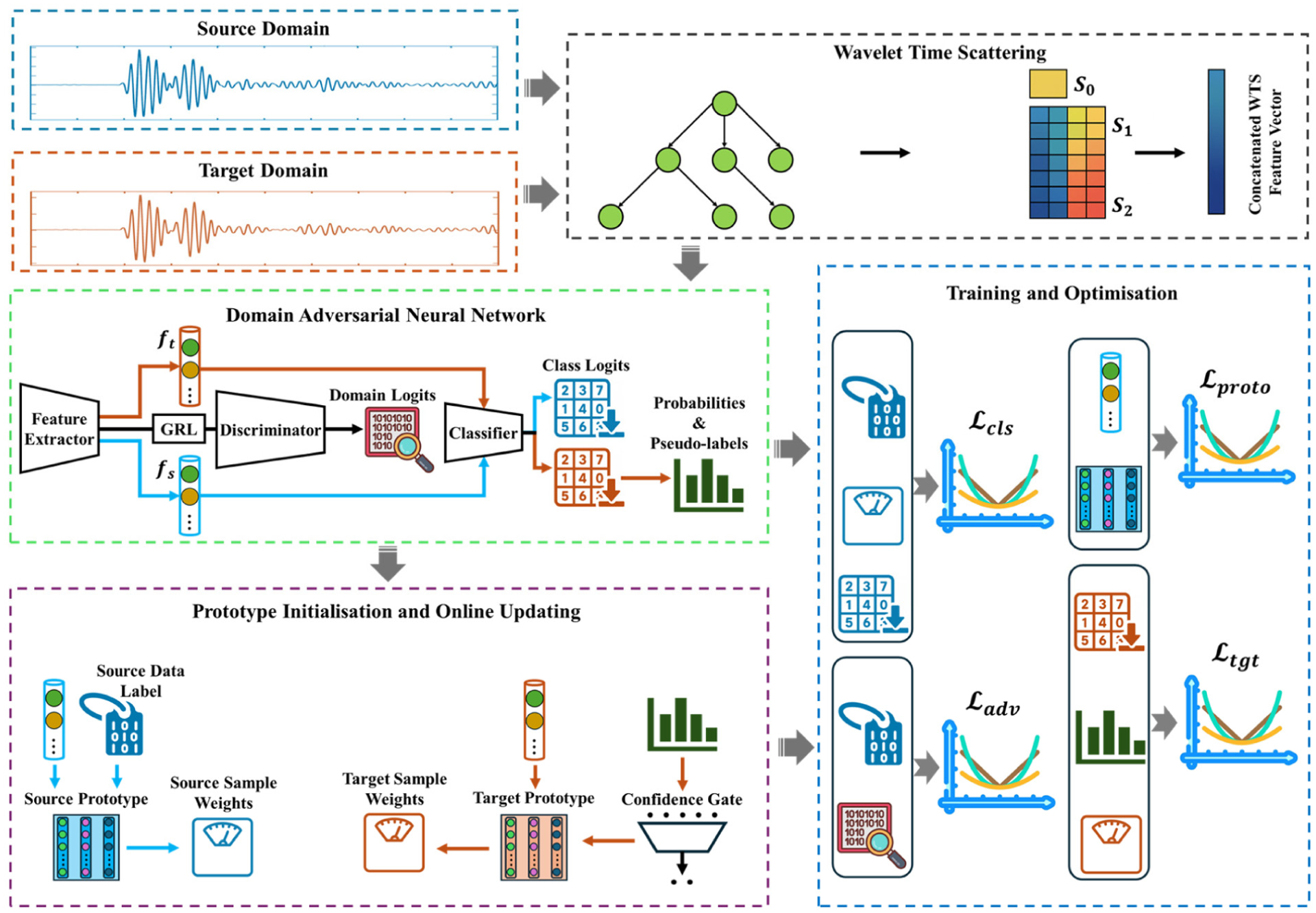
A schematic of SPADA framework. SPADA: scattering-based prototype-aligned domain adaptation.
Interpretability of SPADA internal activity
SPADA incorporates four interpretability views monitoring internal activity to verify source-target latent alignment while preserving class discriminability. These views address WTS features, domain-adversarial latent space, prototype-based attention and unsupervised selection. Crucially, these views serve purely diagnostic purposes without altering training dynamics.
Let
Source labels ensure stable computation despite evolving representations

where
ensuring confident predictions avoid ambiguous sample contamination. Coverage quantifies confident target sample proportion:
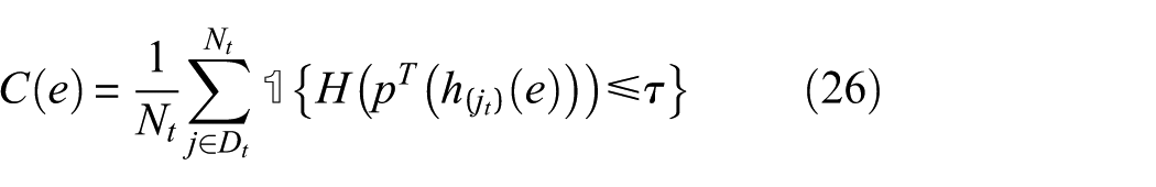
where
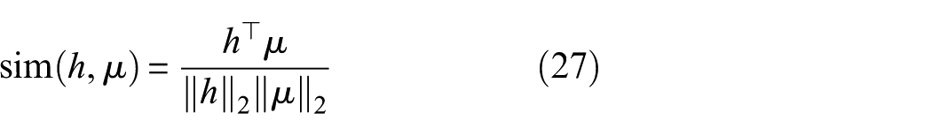
This normalised similarity ranges from −1 to +1, with values near +1 indicating strong alignment. Instance-level attention leverages similarity to modulate sample contribution. Source attention at epoch
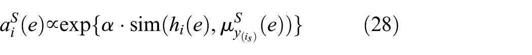
where
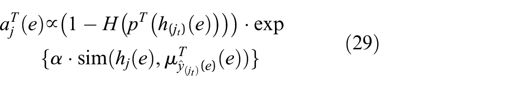
Term
Tracking prototype trajectory evolution
Characterising class structure evolution and target migration towards source centres while preserving inter-class distinctness requires per-class drift and alignment metrics. Source prototype drift quantifies Euclidean displacement between consecutive epochs:

Target prototype drift measures movement:

Alignment gap quantifies distance between source and target prototypes:

Metrics compute independently per class
The trajectory metrics defined above can be interpreted in relation to known physical effects of temperature on structural dynamic response. As demonstrated in the EOV analysis (“Effects of EOVs” section), temperature variation induces systematic changes in wave propagation speed and modal frequencies consistent with thermal softening of the host material. When source and target domains correspond to different temperatures, a reducing alignment gap
Computing instance-prototype cosine similarity
Examining within-class compactness and between-class confusion requires similarity matrix quantifying instance–prototype relationships at selected epochs. For

where
Computation: (1) select analysis epoch
Sharp diagonal block structure in source matrix indicates high similarity to true-class prototypes and low similarity elsewhere, confirming compact, well-separated clusters. Effective adaptation produces similar target patterns: high on-diagonal values for assigned pseudo-label classes and low off-diagonal values. Off-diagonal bands identify confusable class pairs, flagging attention or confidence imbalances. Progressive diagonal enhancement across epochs signals sharpening structure and improving discriminability. Persistent off-diagonal mass on particular classes indicates prototype attractor behaviour, potentially absorbing neighbouring class instances, meriting examination for collapse or overlap.
Monitoring prototype attention weight dynamics
Assessing appropriate target sample weighting and controlled target data reliance growth requires epoch-wise attention weight and coverage summary statistics. Robust statistics avoid outlier sensitivity. For attention weights

where IQR computes as 75th minus 25th percentile difference. Small IQR indicates even attention distribution; large IQR signifies concentration on sample subsets. Median
The whole process can be summarised as: (1) collect target attention weights
Healthy adaptation shows rising or stable
Visualising decision boundaries in feature space
SPADA provides qualitative class separation and source-target overlap visualisation through dimensionality reduction. Projection
Resulting scatter displays source and target instances with distinct markers (circles for source, squares for target), colour-coded by class or pseudo-label. Source prototypes
Excessive invariance manifests as reduced inter-class separation where different-class clusters merge, indicating over-suppression of task-relevant information. Insufficient adaptation produces disjoint source-target clusters within classes, signalling inadequate domain shift mitigation. Alignment between visualisation and quantitative trends in
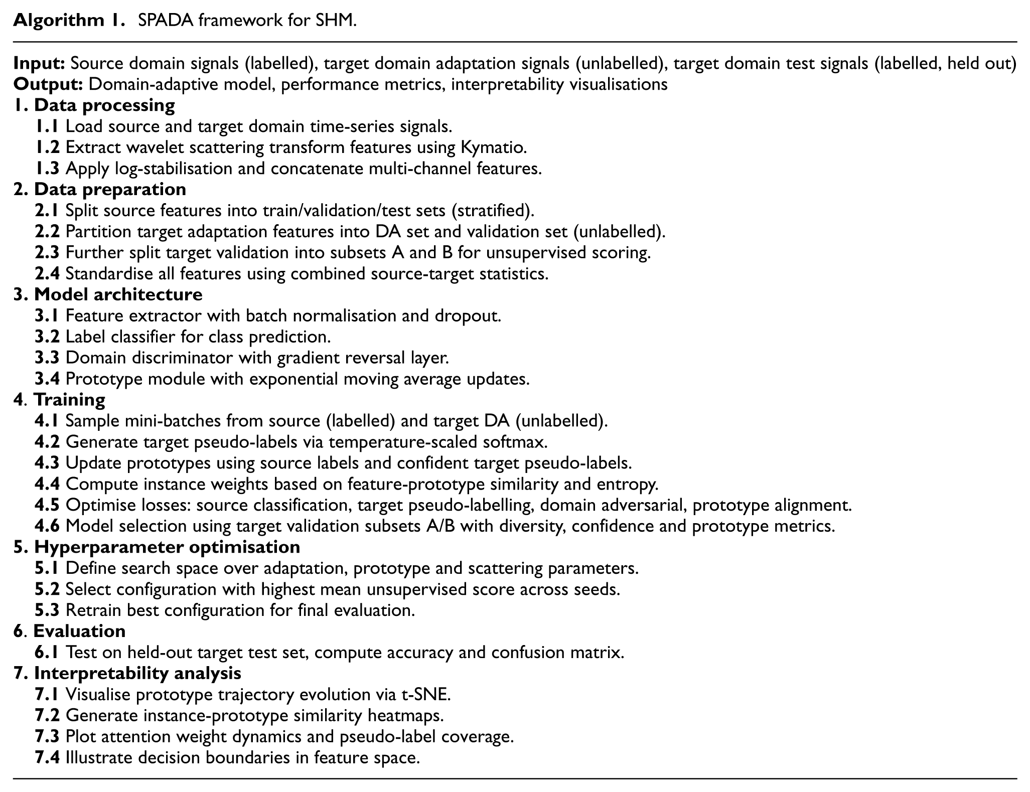
Algorithm 1 presents the algorithm for SPADA.
SPADA framework for SHM.
Case studies
In the present study, two publicly available datasets were employed to assess the effectiveness of the proposed damage detection frameworks. The selection of these datasets was informed by the common experimental setup, in which a temperature chamber was used to regulate the ambient temperature during data collection. In addition, the datasets were derived from two different types of signals, that is, guided wave and vibration signals, thereby enabling a comprehensive evaluation across diverse sensing approaches. The datasets are described in detail in the following sections.
Small-scale WTB under varying climate conditions (WTB-VibClimate)
The first dataset contains experimental signals of a small-scale WTB for the blade of a Windspot 3.5 kW WT model manufactured by Sonkyo Energy disclosed by Qu et al. 32 This blade is made of a three-layered sandwich composite configuration; it has a length of 1.75 m and a mass of 5.0 kg.
Experiments were conducted at 12 temperature conditions from −15 to 40°C in five-degree increments (Wn15, Wn10, Wn5, Wp0, Wp5, Wp10, Wp15, Wp20, Wp25, Wp30, Wp35, Wp40) at 60% humidity. Two excitation modes were applied: white noise (0–400 Hz) and sine sweep (1–300 Hz). Both signals were applied for approximately 120 s with a constant sampling frequency of 1666 Hz at a fixed point on the blade surface. Two sensor types recorded signals: accelerometers and strain gauges, with different configurations. This study used accelerometer data assuming white noise excitation. Although eight sensors recorded data, only three accelerometers (channels 1, 4 and 8) were retained to reduce computational complexity and assess the SHM framework under sensor-limited conditions.
The selection of three from eight available accelerometers was motivated by two considerations. First, it tests the framework under realistic deployment constraints, where cost, cabling and maintenance limit the number of sensors that can be sustained over the operational life of a blade. Second, the three retained channels (1, 4 and 8) span distinct positions along the blade, providing spatial diversity in the captured dynamic response without redundancy from closely spaced sensors. A controlled comparison of the three-sensor and eight-sensor configurations falls outside the scope of the present study, and the reported results should therefore be interpreted as representative of sensor-limited conditions rather than as the upper bound of performance achievable with the full sensor array.
Within the SPADA framework’s WTB-VibClimate case study, these are referenced as channels 1, 2 and 3. Figure 3 shows these accelerometer positions, excitation points and locations of unbalancing mass and cracks on the WTB.
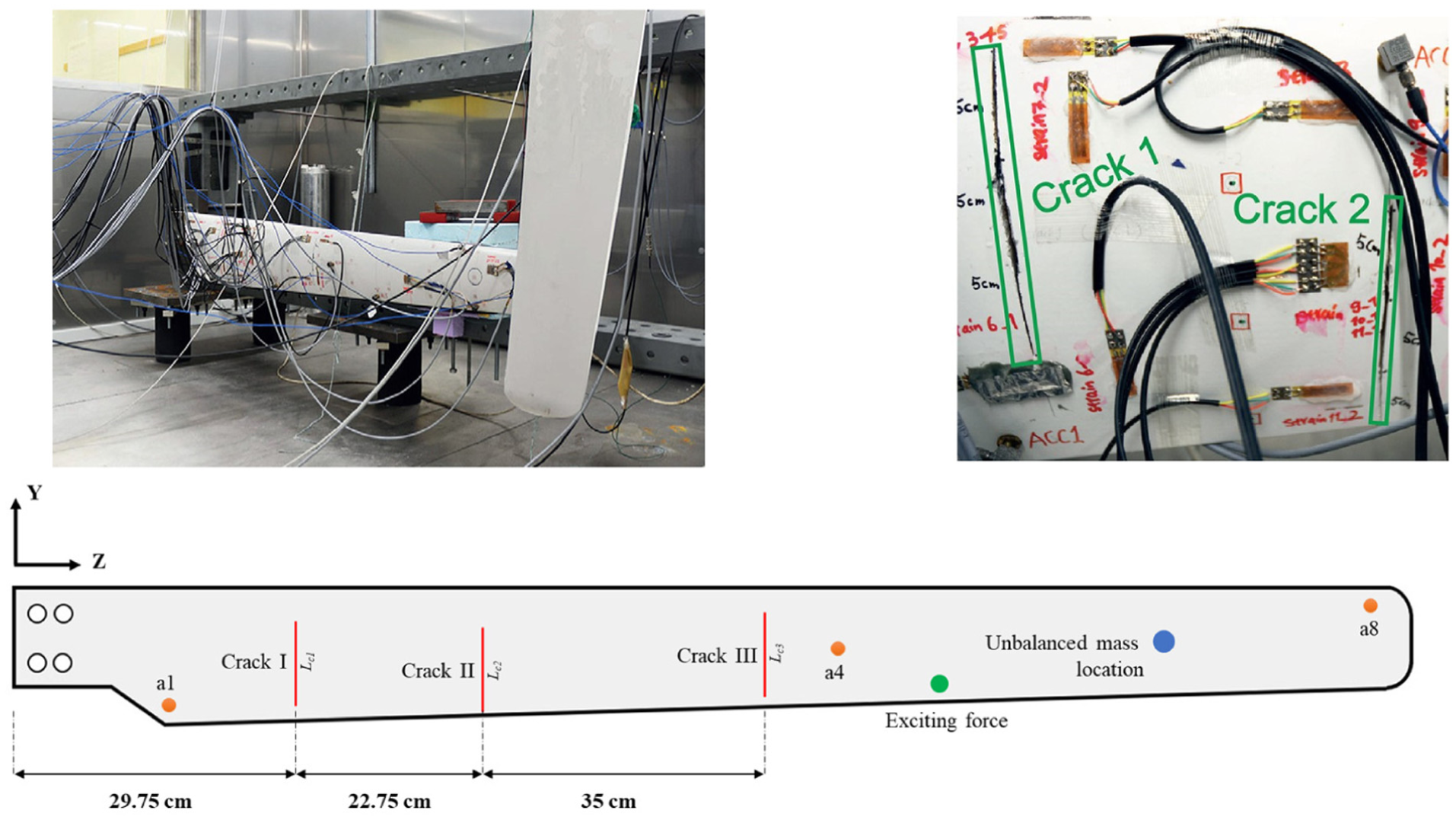
Test rig and sensor configuration in WTB-VibClimate. WTB-VibClimate: small-scale wind turbine blade under varying climate conditions.
Thirteen health scenarios were considered for this WTB: one intact state, nine crack cases (one to three cracks with varying lengths), and three icing scenarios (one to three unbalanced masses of 44 g each). Table 1 summarises these health scenarios with fault quantity and severity; the introduced index is used for classification.
WTB health conditions.
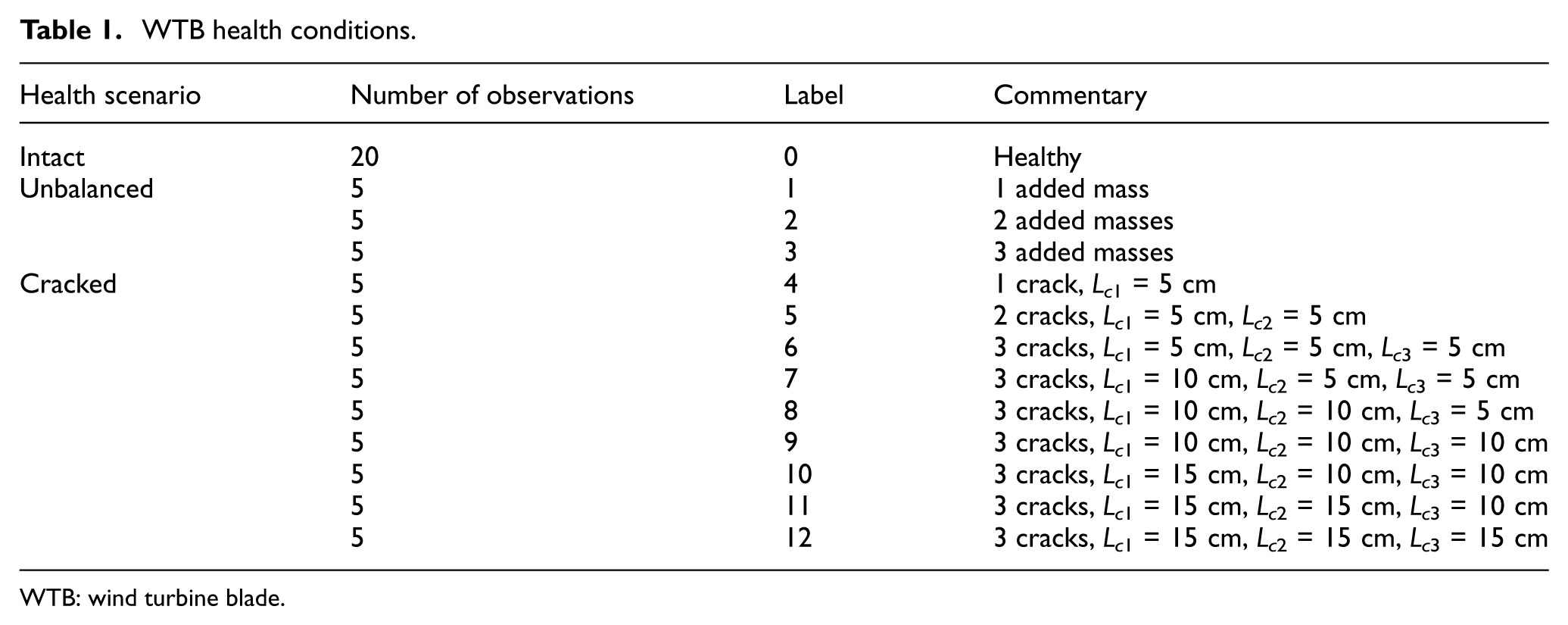
WTB: wind turbine blade.
Carbon–epoxy composite plate
The second dataset, carbon–epoxy composite plate (CONCEPT) 33 contains Lamb wave measurements from a unidirectional carbon-epoxy laminate plate in healthy and damaged states. The experiments investigate how temperature fluctuations and damage progression affect the laminate’s structural behaviour.
Four lead zirconate titanate (PZT) transducers from Acellent Technologies were bonded to the plate. PZT1 acted as the actuator and PZT2, PZT3 and PZT4 as sensors. The plate was tested under free-free boundary conditions to minimise constraints on wave propagation and capture a representative dynamic response. The test rig and instrumentation are shown in Figure 4.
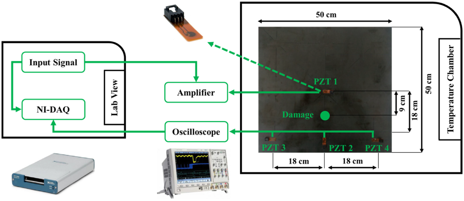
The test rig setup in the CONCEPT test. CONCEPT: carbon–epoxy composite plate.
The experiments were conducted in a Thermotron thermal chamber to provide precise temperature control using an integrated cascade refrigeration system, so that 0°C was reached by mechanical cooling rather than ambient freezing. A sinusoidal tone burst served as the excitation signal, and the responses were sampled using dedicated data acquisition systems operated via LabVIEW. For the intact plate, 100 measurements were collected at each of seven temperature levels from 0 to 60°C, labelled Cp0, Cp10, Cp20, Cp30, Cp40, Cp50 and Cp60. For the damaged plate, 100 measurements were acquired only at 30°C, which served as the baseline, with no damaged data at other temperatures.
Damage scenarios were simulated by applying industrial adhesive putty to the plate surface to create delamination-like defects. The damage severity was progressively increased in a localised region between PZT1 and PZT2 to study the resulting changes in wave attenuation and propagation. Table 2 summarises the health scenarios, their severities and brief descriptions, and reports the labels assigned to the different temperatures.
Damage scenarios and severities for simulated defects in the CONCEPT experiment.
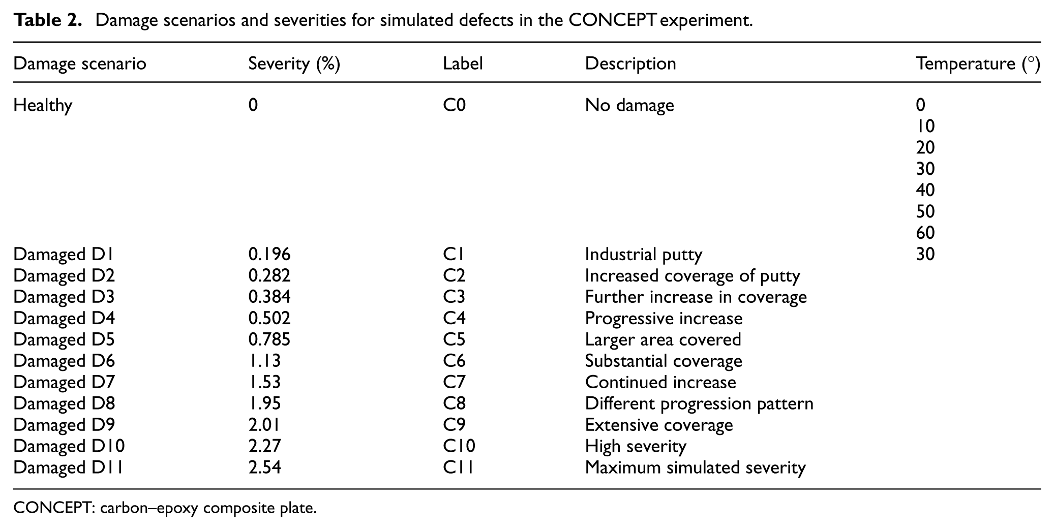
CONCEPT: carbon–epoxy composite plate.
Results and discussion
This section presents the effects of EOVs on guided wave and vibration signals. Data augmentation results are discussed through two standard metrics. Results with and without the SPADA domain-adaptation stage are compared. The internal activities of SPADA throughout DA are examined. The applied feature extraction methods and the effects of domain shift on extracted features are presented and compared with convolutional neural networks (CNNs).
Effects of EOVs
Because EOVs mainly alter stiffness, damping and wave-propagation speed in the monitored structure, its influence is often not apparent in raw time-domain signals. More diagnostic representations are therefore required, such as frequency-response functions (FRFs),
34
mode shapes and coda wave interferometry (CWI).
35
In FRF analysis, the structural response to a known input is expressed in the frequency domain as
Method suitability depends on actuation and sensing capabilities, wavefield properties, linearity, access constraints, computational cost and baseline availability. For composite plates with PZT-guided waves, FRF approaches fail because bonded PZTs provide distributed frequency-dependent tractions, dispersive multi-modal fields mix modes in single-input-output measurements, closely spaced lightly damped modes require dense sampling and temperature drifts violate time-invariance. Wavefield-based methods like CWI are more effective. In this section, mode-shape and FRF analyses were applied to the low-frequency vibration responses in WTB-VibClimate, while CWI was used for the guided-wave measurements in CONCEPT.
WTB-VibClimate
The purpose of this analysis is to quantify how temperature affects mode shapes and FRFs of the WTB-VibClimate system. FRFs were estimated in MATLAB® using the H1 estimator from healthy measurements at all temperatures labelled Wn15 to Wp40. For each temperature, 20 runs were processed with channel 1 as the response and the force channel as the input. Signals were trimmed by discarding the first 10,000 and last 20,000 samples, then detrended and band pass filtered between 0.5 and 380 Hz using a zero-phase finite impulse response filter of order 800. Spectral estimates for FRF computation used Welch’s method with a sampling rate of 1666 Hz, a Hann window of 4 s, 50% overlap and a fast Fourier transform length of 8192.
FRFs from repeated runs were then pooled using weights proportional to the squared coherence, retaining only frequency bins with squared coherence at or above 0.8 for averaging, while plots were masked below 0.7. Modal candidates at the 10°C baseline were identified by peak picking with at most four modes, minimum peak prominence 3% of the baseline maximum, minimum inter-peak spacing 1 Hz and matching tolerance 1 Hz for ridge initialisation. Modal ridges were tracked across temperatures within non-overlapping frequency bands around the baseline peaks, and half power bandwidth calculations yielded damping estimates for each mode. When multiple response channels were available, mode shapes were obtained from the complex FRFs at each modal peak and normalised across channels at the baseline, with an optional output only frequency domain decomposition check based on the first singular value of the response spectral density matrix. The corresponding mode shape plots and FRF maps are presented in Figure 5(a) and (b), respectively.
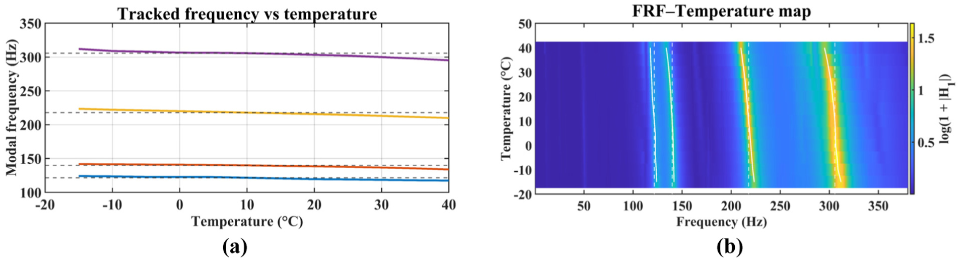
(a) Mode shapes identified at the baseline temperature of 10°C, based on normalised FRFs and (b) FRF–temperature maps for the WTB-VibClimate dataset showing the variation of response magnitude across temperature levels. FRF: frequency-response function; WTB-VibClimate: small-scale wind turbine blade under varying climate conditions.
Figure 5(a) shows four modal frequencies that are highest at −15°C and decrease approximately linearly as temperature rises to +40°C. The largest shift occurs near 300 Hz, with a smaller but clear shift around 215–220 Hz and more modest changes near 140 and 120 Hz, strongest for the two highest frequency modes. The dashed horizontal markers indicate the 10°C baseline, with the curves above the baseline at sub-zero temperatures and below it at warmer conditions. Figure 5(b) confirms these trends: bright FRF ridges remain in the same modal bands but migrate to lower frequency with increasing temperature, and their slight thickening and reduced intensity at higher temperatures suggest modest peak broadening consistent with increased damping. No mode crossing is observed, so mode ordering is preserved. Together, the figures show a systematic temperature dependence of the dynamic response, consistent with thermal softening, which motivates temperature compensation when using these data for classification.
Concept
For the CONCEPT guided-wave data, temperature-induced EOVs were quantified using CWI. A baseline at 30°C was formed by median-stacking the kept runs, and for each temperature level (0–60°C) every observation that passed force-channel quality screening was pre-processed (detrending and zero-phase band-pass filtering around the burst) and compared against the baseline through a stretch-correlation search over
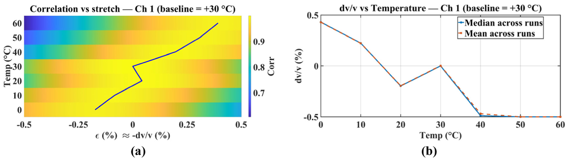
(a) CWI correlation–stretch map and (b) fractional wave-speed change versus temperature for CONCEPT. CWI: coda wave interferometry; CONCEPT: carbon–epoxy composite plate.
From Figure 6(a), similarly, it can be understood that the ridge of maximum correlation,
Analysing Figure 6(b), one can observe that a clear, near-monotonic decrease in
Data augmentation
The two different data augmentation techniques, that is, signal windowing and Conv-CVAE implemented on WTB-VibClimate and CONCEPT case studies, respectively, are elaborated in the following.
Signal windowing
A windowing strategy expanded the WTB-VibClimate dataset, feasible given uniform sampling. Each observation was divided into five equal 39,200-point segments. To avoid edge effects, the first 4000 data points and the 4000 last data points were excluded, resulting in 196,000 clean points divided into five non-overlapping windows. This produced 25 observations per damaged condition. The same procedure was applied to the healthy condition (using the first five original observations). With 13 health scenarios, this generated a 325 × 3 × 39,200 dataset per temperature level. To prevent data leakage, 15 target-domain observations (from three original recordings) were allocated for DA, while 10 observations (from two separate recordings) remained entirely unseen for testing.
A methodological caveat applies to the windowing procedure. Because all windows from a given original recording share the same excitation event, boundary conditions and sensor coupling state, they are not statistically independent realisations. The reported uncertainty, therefore, reflects variability due to random data splits and model initialisation rather than variability across independent experimental repetitions. This distinction does not invalidate the reported accuracies, which remain valid point estimates of classification performance on the held-out windows, but it means that the associated confidence intervals may underestimate the true variability that would be observed across fully independent measurement campaigns. Future work should incorporate recording-level resampling or leave-recording-out cross-validation to provide uncertainty estimates that account for this dependence structure.
Conv-CVAE
Conv-CVAE as a temperature-conditioned generative augmentation method was implemented in PyTorch to augment CONCEPT. The model was trained for 150 epochs with batch size 128, latent dimension 64, learning rate
The composite loss weights were set to
The Gaussian smoothing kernel for the amplitude masks used
The encoder comprised three one-dimensional convolutional layers (filters 7, 5, 5; stride 2) with batch normalisation and GELU activations; the decoder used mirrored transposed convolutions. Temperature was encoded as a normalised scalar concatenated at fully connected layers. For each of 12 damage levels, a latent offset vector was computed at reference temperature Cp30. Per-sensor and per-time amplitude masks derived from Hilbert envelopes used Gaussian-smoothed median ratios (
Loss combined mean squared error (MSE), log-magnitude fast Fourier transform (FFT) spectral terms, wavelet similarity (four-level Daubechies-4), envelope consistency and Kullback–Leibler (KL) divergence
Damaged signals at temperature
To examine the extent to which the synthesised signals replicate the behaviour of the experimental data, two quantitative metrics were employed: dynamic time warping (DTW) 36 and cross correlation (CC). 37 A lower DTW (ideally 0) value and |CC| close to 1 indicates strong similarity between the synthesised and original data. The data were generated for the baseline temperature of 30°C, which includes observations from all health scenarios. For each condition, 50 observations were used to produce the synthesised data, while the remaining 50 observations per class were retained for comparison with the corresponding synthesised signals. This approach ensured a balanced and consistent evaluation process. The results are shown in Figure 7.
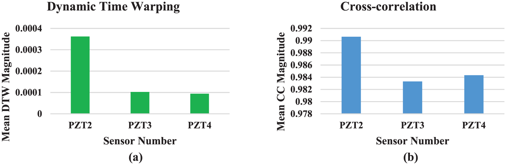
Comparison of synthesised data (through Conv-CVAE) and real data across sensors (PZT2, PZT3, PZT4) for Cp30 using (a) mean DTW values and (b) mean CC values. PZT: lead zirconate titanate; DTW: dynamic time warping; CC: cross correlation.
Observing Figure 7, Conv-CVAE demonstrates strong agreement at Cp30. Mean DTW values are extremely low, that is, PZT2 (0.000362), PZT3 (0.000103) and PZT4 (0.000094) while CC values remain high: PZT2 (0.990627), PZT3 (0.983301) and PZT4 (0.984319). Conv-CVAE’s low DTW value and high (near to 1) CC magnitude reflect its capacity to capture non-linear temporal variations through temperature-conditioned latent representations and learned amplitude and phase masks.
For the Conv-CVAE–generated damaged scenario C11, CWI was deployed to assess whether the temperature-induced EOV behaviour in the synthetic responses remains consistent with that observed on the experimental healthy plate. Temperature-induced EOV was quantified using the same CWI configuration as in the healthy CONCEPT analysis, except that the force-channel–based quality screening could not be applied because excitation traces are not available for the synthesised data. For each temperature level (0–60°C), all 30 synthesised observations for each PZT were pre-processed and compared with the 30°C damaged baseline; run-wise
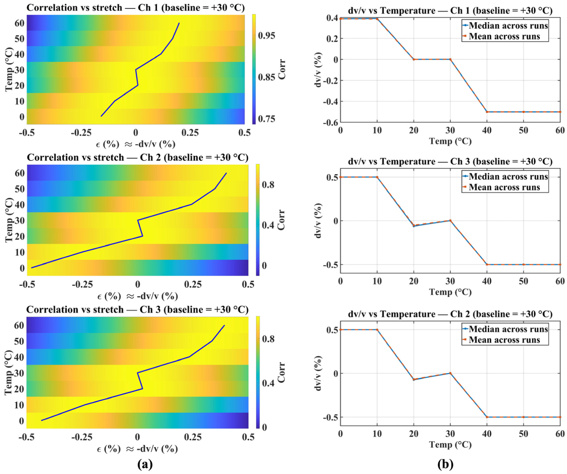
CWI results for the Conv-CVAE–synthesised damaged case C11 in CONCEPT: (a) correlation–stretch map; (b) fractional wave-speed change
The
To provide indirect validation of Conv-CVAE synthesis fidelity beyond the DTW and CC metrics reported at Cp30, bidirectional cross-classification was conducted using a Random Forest classifier with 200 trees. Training on real Cp30 data with 1200 observations and testing on synthetic data with 360 observations achieved 81.67% accuracy, whereas the reverse direction achieved 75.50%. These moderate accuracies indicate a distributional gap at the raw-waveform level, where the classifier must resolve fine inter-class boundaries that the Conv-CVAE does not replicate perfectly. However, per-class cross-correlation remained above 0.98 for all 12 damage classes, with a mean CC of 0.991, confirming that the dominant waveform morphology and damage-severity ordering are preserved. The contrast between high CC and moderate cross-classification accuracy is consistent with the SPADA pipeline design, since the Conv-CVAE is not intended to generate waveform-identical copies, but rather to generate signals whose WTS features preserve class-discriminative structure across temperatures.
Damage detection
To assess SPADA’s effectiveness in detecting damage under EOVs, two case studies (WTB-VibClimate and CONCEPT) were analysed separately. This section presents results from intermediate and final evaluation stages, including damage detection without DA and with complete SPADA. Ablation and comparative studies were conducted for both cases. Internal SPADA activities were visualised to demonstrate domain adjustment for EOV mitigation, and computational efficiency was evaluated for real-time deployment capability.
Unless otherwise stated, all reported target-domain accuracies correspond to the mean across 15 independent seeds for the selected configuration, rather than the single highest accuracy across seeds.
WTB-VibClimate
To evaluate SPADA’s performance on small-scale WTB damage detection, the augmented WTB-VibClimate dataset was employed following the windowing procedure. To prevent test-set leakage during DA, 10 samples (from two original observations) were reserved for testing, while 15 samples (from three originals) were allocated for training and validation: 11 for DA and 4 for unsupervised validation. This stratified allocation ensured class balance and complete separation between adaptation and testing data.
Feature extraction
SPADA utilised a high-level WTS to extract discriminative features. Each channel was standardised to remove mean offsets and normalise variance. The scattering transform employed Morlet wavelets, suitable for vibration analysis due to their balanced frequency localisation and time resolution, capturing transient and oscillatory behaviours.
38
The transform used maximum scale
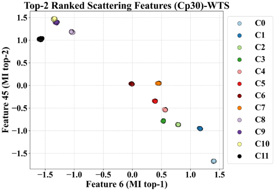
Scattering coefficients underwent logarithmic compression to reduce large fluctuations and enhance stability. Temporal averaging produced fixed-length, time-shift-invariant descriptors sensitive to oscillatory structure. Features from three sensor channels were concatenated to form unified representations. WTS resulted in compact, translation-invariant, noise-robust features preserving fine-scale transients and broader structural variations, providing reliable input for subsequent DA and classification. To evaluate feature extraction efficacy, scattering transforms were applied to three-channel vibration signals at Wp20 (representative operational condition). Features were extracted per channel, normalised, temporally averaged, and concatenated. The top two features ranked by mutual information are visualised in Figure 9.
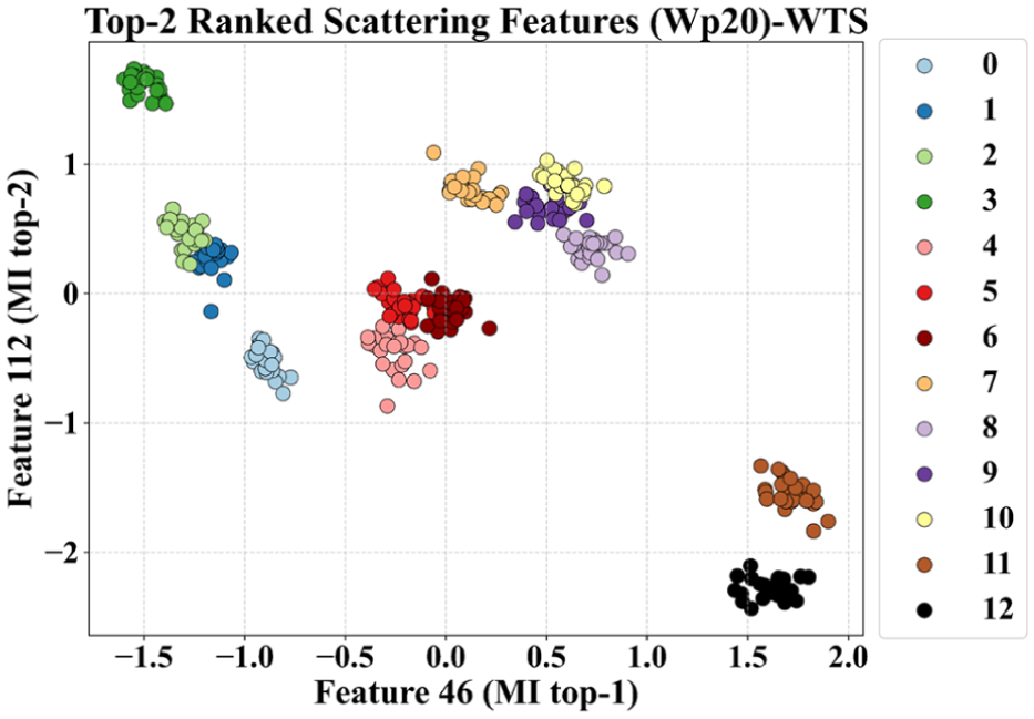
Scatter plot of the top-2 features ranked by mutual information, based on scattering transforms employed on Wp20; samples are colour-coded by labelled classes (Table 1).
Figure 9 shows effective separation across classes. However, overlap persists between crack-related classes 5 and 6, and classes 9 and 10, likely from subtle crack characteristic differences (length, severity) harder to distinguish in 2D projections but linearly separable in full feature space.
To examine EOV impact on data distribution and assess WTS’s domain-invariant feature capture, scatter analysis used three datasets (Wn15, Wp20, Wp40). The two most discriminative MI-ranked features appear in Figure 10(a). For comparison, WTS was substituted with a CNN comprising four one-dimensional convolutional layers with batch normalisation, ReLU activations, global average pooling, and linear projection to 64-dimensional embedding space. The CNN was trained in a supervised manner on source-domain data. The same three datasets were processed, with top-ranked features in Figure 10(b). Features were ranked using Wp20 for consistency with Figure 9; five observations per class per domain were plotted for visibility.
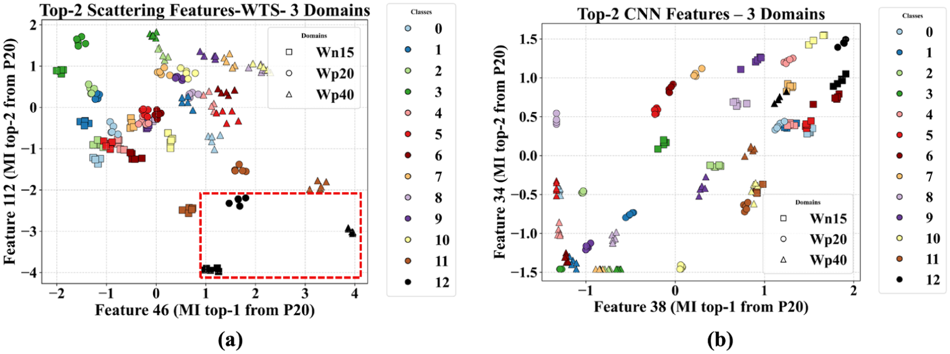
Scatter plot of the top-2 features ranked using Wp20 data, visualised across three temperature conditions (Wn15, Wp20, Wp40); for (a) WTS-based and (b) CNNs-based feature extraction. WTS: wavelet time scattering; CNN: convolutional neural network.
In Figure 10(a) (WTS), class clusters exhibit clear domain-wise ordering: Wn15 samples consistently left, Wp20 centred, Wp40 right along the first MI feature, with this left-centre-right pattern repeating across classes while preserving intra-class compactness (red-dashed rectangular). WTS encodes temperature shifts as approximately monotonic displacement in feature space while maintaining class structure, conducive to cross-domain alignment. Conversely, Figure 10(b) (CNNs) shows weaker domain regularity and greater intermingling of temperature samples within class groups despite comparable separability, suggesting the Wp20-trained CNN captures class-discriminative cues but with reduced domain awareness and poorer EOV alignment as will be discussed in the subsequent sections.
A one-dimensional ResNet-18 variant (ResNet1D) was additionally evaluated as a deeper learned backbone. The architecture comprised a convolutional stem (kernel size 7, stride 2, 64 channels, batch normalisation, ReLU, max-pooling with kernel size 3 and stride 2), followed by four residual stages of two BasicBlock1D modules each, with output channels of 64, 128, 256 and 512 and stride-2 downsampling at the first block of stages 2 through 4. Skip connections in downsampled blocks used a 1 by 1 convolution for dimension matching. Global average pooling and a linear projection with dropout (0.2) produced a 64-dimensional embedding. The network was trained in a supervised manner on source-domain data using the same protocol as the CNN baseline. The effects of this feature extraction technique on the damage detection also will be discussed on WTB-VibClimate as well as CONCEPT in the following sections.
Damage detection without DA
Damage detection was conducted assuming no DA stage; 3 temperatures (Wn15, Wp20, Wp40) were independently designated as source domains, with remaining datasets as targets. DA loss weights (
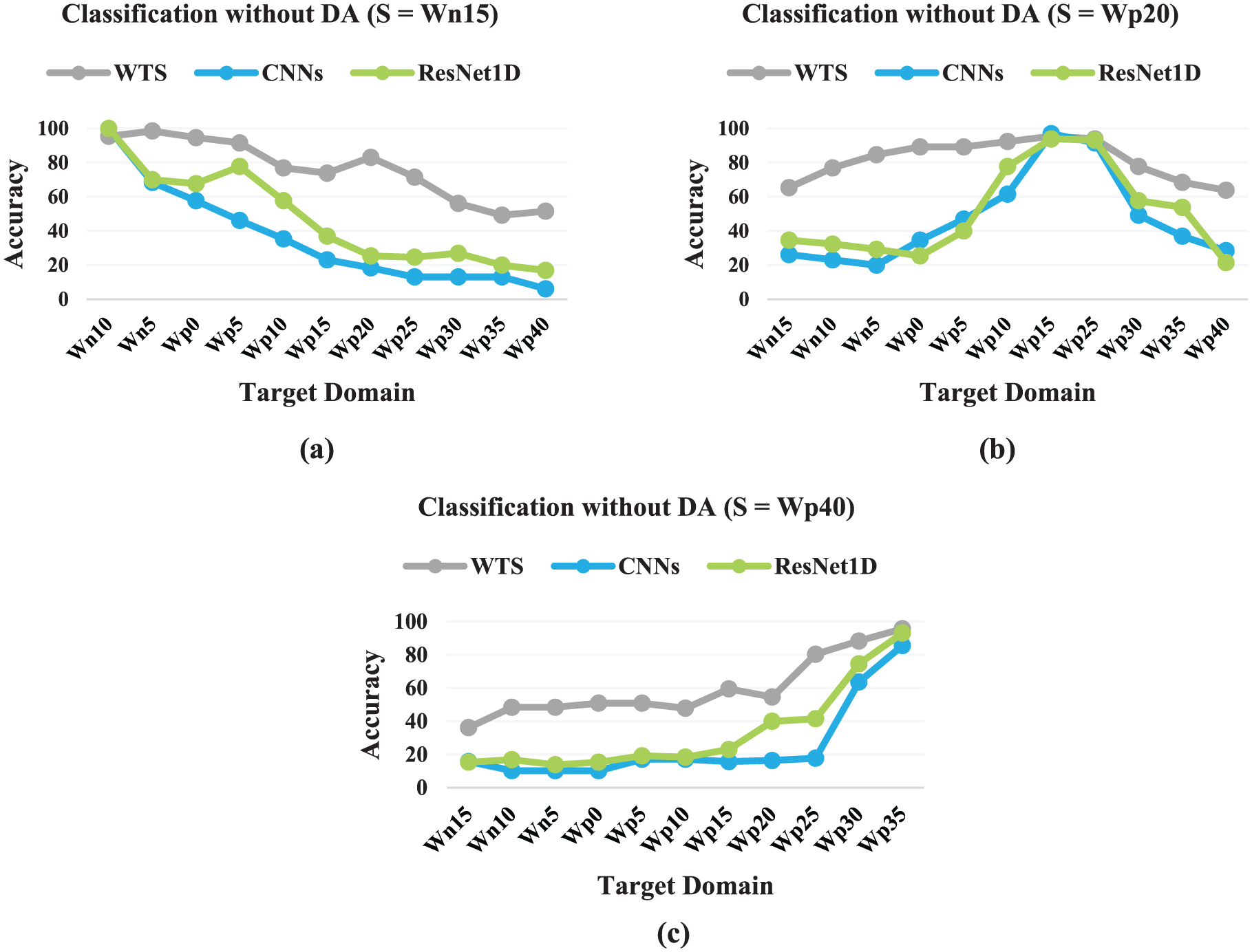
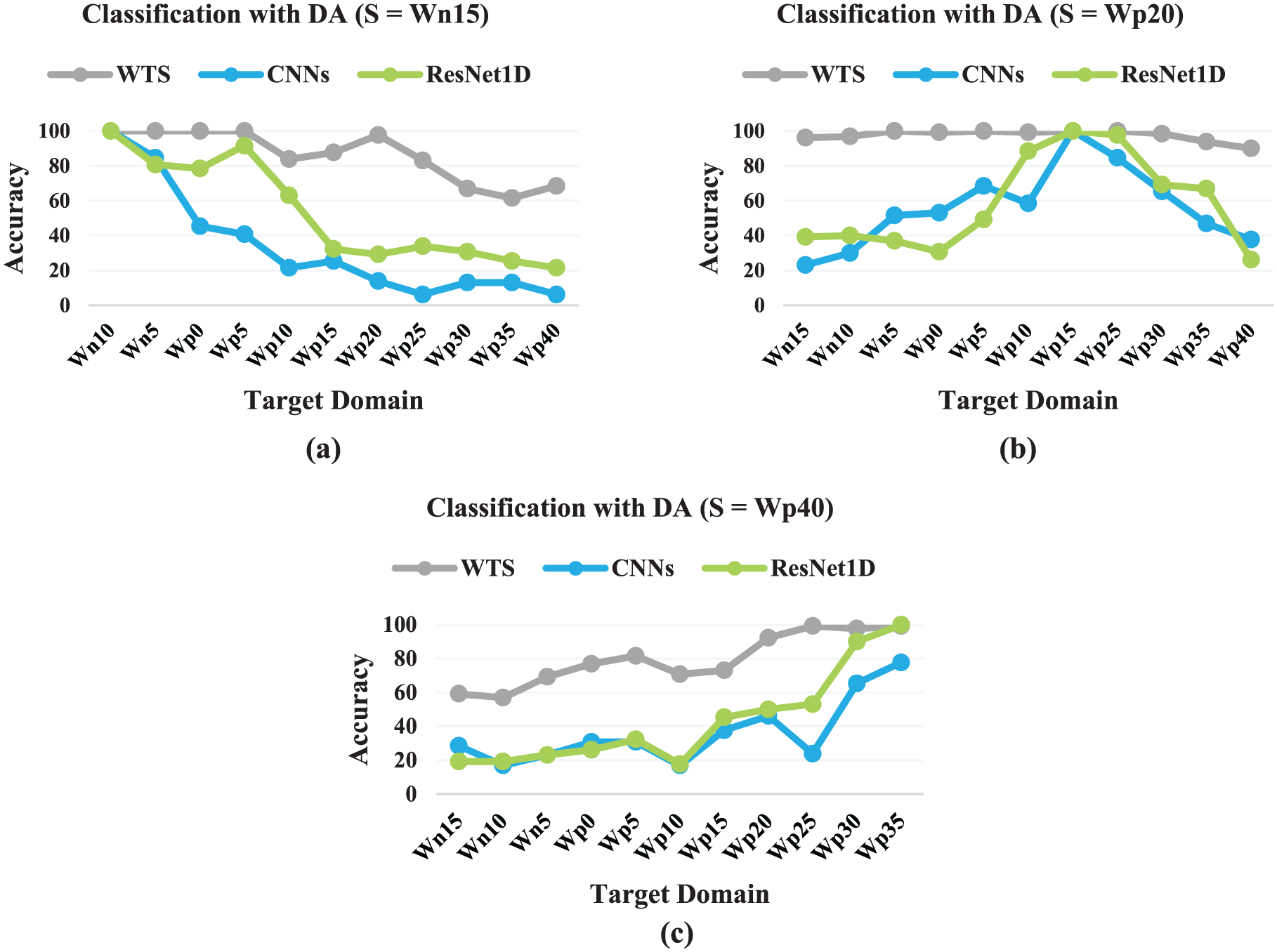
Damage detection utilising WTS, CNNs and ResNet1D without DA when (a) Wn15, (b) Wp20 and (c) Wp40 was assigned as the source domain. WTS: wavelet time scattering; CNN: convolutional neural network; DA: domain adaptation.
Figure 11 reveals clear temperature proximity effects. Using WTS, average accuracies across targets were 76.57% (Wn15 source), 81.54% (Wp20) and 60.0% (Wp40). Corresponding CNN averages were markedly lower: 35.87, 46.85 and 25.24%. Wp20 consistently provided strongest generalisation for both methods.
WTS degraded gracefully as source-target temperature gaps widened, while both learned backbones were markedly more sensitive to mismatch. With Wp20 as source, average accuracies across targets were 81.54% (WTS), 50.84% (ResNet1D) and 46.85% (CNN). With Wn15 as source, corresponding averages were 76.57% (WTS), 47.62% (ResNet1D) and 35.87% (CNN). With Wp40 as source, averages were 60.0% (WTS), 33.78% (ResNet1D) and 25.24% (CNN). ResNet1D consistently outperformed the shallower CNN but remained substantially below WTS across all source settings, indicating that increased network depth alone does not compensate for the absence of the translation-invariance and deformation-stability properties that WTS provides.
Persistently lower accuracies at larger temperature differences indicate systematic generalisation gaps, strongly justifying DA incorporation to mitigate temperature-induced covariate shift and stabilise performance across dissimilar operating conditions.
Damage detection with DA
To address detection gaps under large temperature differences, full SPADA with DA was deployed. Hyperparameters were tuned via random search over 1000 configurations without replacement. For each configuration, 15 independent seeds were run. All 15 seeds were executed for every sampled configuration, not only for the final selected configuration. This ensures that the mean unsupervised score used for configuration selection reflects the full seed-level variability of each candidate, rather than being estimated from a single run. Epochs were selected using the unsupervised two-part hold-out score on unlabelled target validation subsets A and B, as described in the training summary. Models were retrained with the chosen configuration under the same 15 seeds; test performance was reported based on the mean accuracy on held-out target test sets. Reproducibility was ensured by controlling all randomness sources: seeds were applied consistently to Python, NumPy, PyTorch and scikit-learn, with deterministic data loading, shuffling and augmentation. Target-domain data used in DA was fixed at 60% class-balanced proportion; consequently, 10 observations per class were allocated to testing.
In WTS, maximum scale was constrained to
Hyperparameter candidates and values in SPADA.
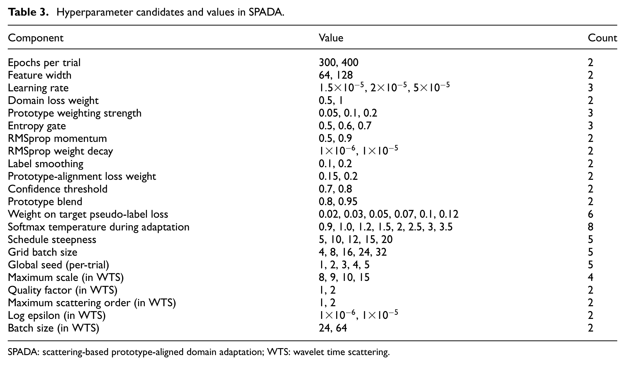
SPADA: scattering-based prototype-aligned domain adaptation; WTS: wavelet time scattering.
The unsupervised selection score used fixed combination weights
Following the without-DA scenario, three source-to-target settings were considered. Figure 12(a) to (c) presents highest target accuracies, with CNN and DA results plotted for comparison.
Damage detection utilising WTS, CNNs and ResNet1D with DA when (a) Wn15, (b) Wp20 and (c) Wp40 was assigned as the source domain. WTS: wavelet time scattering; CNN: convolutional neural network; DA: domain adaptation.
With Wp20 as source (Figure 12(b)), accuracies were uniformly high, averaging 97.58%. With Wn15 as source (Figure 12(a)), perfect results occurred for nearby targets, but performance decreased for hottest targets (Wp30 66.92%, Wp35 61.54%), averaging 86.29%. With Wp40 as source (Figure 12(c)), coldest targets were most challenging (Wn10 56.92%, Wn15 59.23%), while warm targets remained strong, averaging 79.65%. Comparing to Figure 11 (without DA), averages increased from 35.87, 46.85 and 25.24% to 86.29, 97.62 and 79.65%, indicating earlier low-accuracy gaps were largely closed. For instance, Wn15 to Wp35 increased from 13.08 to 61.54%.
Both learned backbones with DA achieved lower accuracies than WTS with DA. ResNet1D with DA improved over its without-DA baseline (averages rising from 50.84 to 58.60% with Wp20, from 47.62 to 53.36% with Wn15 and from 33.78 to 43.29% with Wp40), confirming that the adaptation mechanism provides benefit even with deeper learned features. CNN with DA showed similar but smaller gains, and in some transfers, performance fell below without-DA settings, reflecting negative transfer. Nonetheless, both learned backbones with DA remained substantially below WTS with DA (97.58, 86.29 and 79.65% for the three source settings), reinforcing that the stability properties of WTS features facilitate more effective domain alignment than representations optimised purely for source-domain discrimination.
To understand which classes SPADA (with DA) struggles to classify, confusion matrices are presented for 4 target domains (Wn10, Wp0, Wp30, Wp35) in Figure 13(a) to (d), respectively, assuming Wp20 as source. These targets were selected because SPADA did not achieve full accuracy, allowing detailed limitation examination.
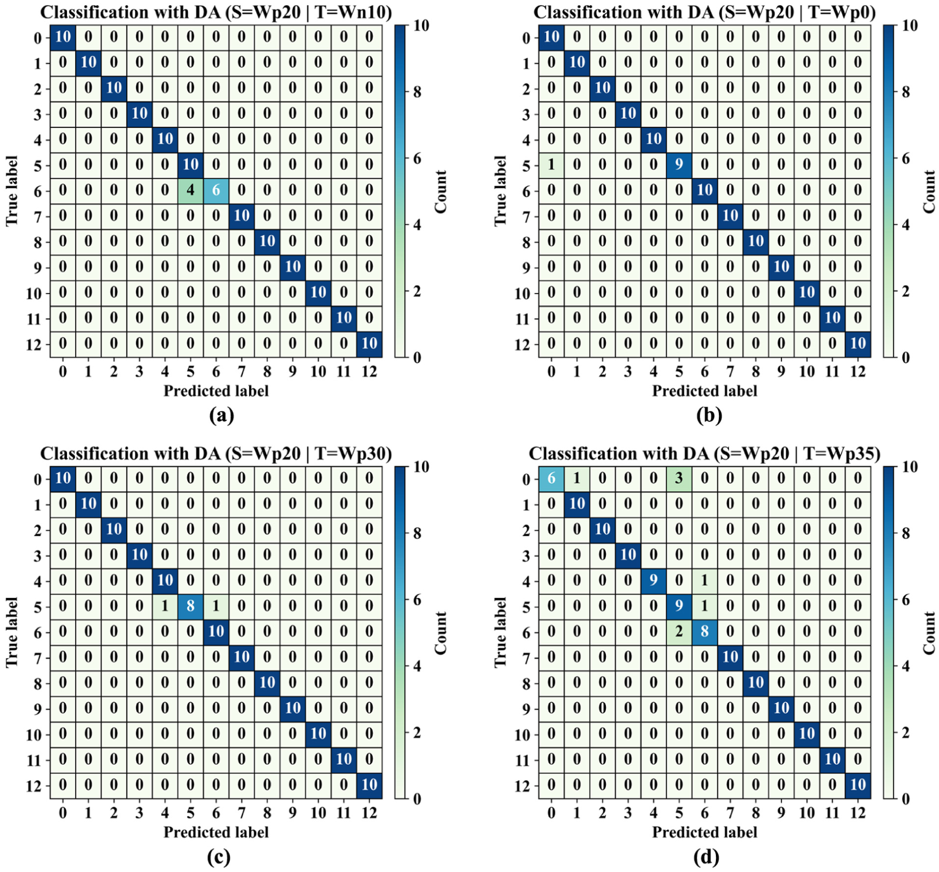
Confusion matrices of SPADA with Wp20 as the source and (a) Wn10, (b) Wp0, (c) Wp30 and (d) Wp35 as target domains. SPADA: scattering-based prototype-aligned domain adaptation.
Figure 13 shows SPADA’s residual errors concentrate almost entirely in pairwise confusions between labels 5 and 6; misclassifications are symmetric and limited, indicating tight decision boundaries rather than widespread class drift. These labels correspond to closely related crack configurations (two vs three 5 cm cracks), inducing similar stiffness reductions and mode-shape perturbations. Under temperature shift, spectral signatures become more alike due to thermal softening and peak broadening, narrowing margins between class prototypes. Effects are amplified by (i) sensor-limited operation (three channels), reducing spatial sensitivity to crack multiplicity; (ii) windowed segmentation, preserving local transients but weakening global geometry cues; and (iii) conservative pseudo-labelling during adaptation, slightly relaxing class margins for near-neighbour classes.
To address safety-relevant diagnostic performance, per-class recall was computed for all transfer pairs with Wp20 and Wn15 as source domains. Figure 14 presents these values as heatmaps, where rows correspond to target transfers and columns to health-scenario classes. Since the false negative rate is the complement of recall (False Negative Rate = 1 − recall), only the recall heatmaps are shown. With Wn15 as source (Figure 14(a)), a clear gradient emerges: nearby targets retain high recall across all classes, while distant targets (Wp25 to Wp40) exhibit reduced recall for mid-severity crack classes (4–9), reflecting the compounded difficulty of distinguishing closely related damage configurations under large thermal shifts. With Wp20 as source (Figure 14(b)), recall remains at or near unity across the majority of transfers and classes; the only visible degradation concentrates on classes 5 and 6 at the widest temperature gaps (Wp35 and Wp40), consistent with the pairwise crack-configuration confusion identified in the confusion matrices. Because all health scenarios contain equal numbers of observations, the macro-averaged F1 score is numerically close to the overall accuracy for each transfer pair and is therefore not reported separately.
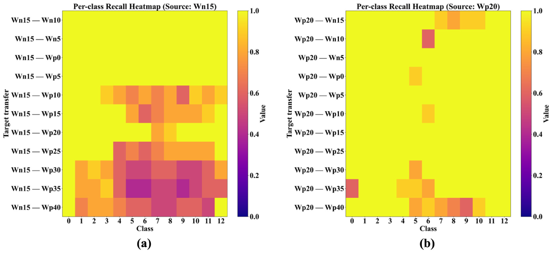
Per-class recall heatmaps for WTB-VibClimate with DA: (a) Wn15 and (b) Wp20 as source domain. WTB-VibClimate: small-scale wind turbine blade under varying climate conditions; DA: domain adaptation.
Concept
Before presenting the CONCEPT adaptation results, it is important to note that this case study constitutes a constructed evaluation setting: healthy signals are experimental across all seven temperatures, while damaged signals at non-baseline temperatures are synthetic, generated by the Conv-CVAE described in previous sections. Consequently, performance figures for CONCEPT transfers reflect the combined effect of the adaptation mechanism and the generator fidelity, and should not be interpreted as evidence of robustness against experimentally measured damaged responses at varying temperatures. Direct experimental support for cross-temperature robustness is provided by the WTB-VibClimate results, where real damaged data exist at all temperature conditions.
SPADA was evaluated on composite plate damage detection using the CONCEPT dataset augmented with synthetic damaged signals generated by the convolutional conditional variational autoencoder. To avoid DA bias, the baseline temperature dataset (Cp30), which contains the only experimentally measured damaged signals, was excluded and used only for scatter plots. Only Cp0, Cp10, Cp20, Cp40, Cp50 and Cp60 were considered. Two scenarios were examined: (1) Cp0 (lowest temperature) as source with remaining temperatures as targets and (2) Cp60 (highest temperature) as source with others as targets.
During DA, 50% of target data were allocated for training, 50% for testing (class-balanced, randomly selected). Consequently, 15 observations per class were classified in testing.
Feature extraction
The same WTS block from WTB-VibClimate was employed, with maximum scale limited to
Scatter plot of the top-2 features ranked by mutual information, based on scattering transforms employed on Cp30; samples are colour-coded by labelled classes (Table 2).
Figure 15 demonstrates successful WTS class separation. However, meaningful class hierarchy must also be maintained under temperature variation. Figure 16(a) and (b) present 2D scatter plots of MI-ranked features for three domains (Cp0, Cp30, Cp60) using WTS and CNNs, respectively. CNNs used the same supervised framework as WTB-VibClimate; five observations per health scenario per domain were plotted.
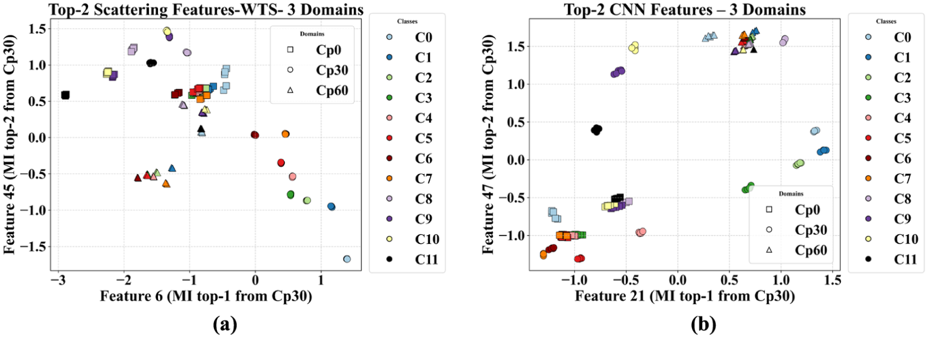
Scatter plot of the top-2 features ranked using Cp30 data, visualised across three temperature conditions (Cp0, Cp30, Cp60); for (a) WTS-based and (b) CNNs-based feature extraction. WTS: wavelet time scattering; CNN: convolutional neural network.
Figure 16 shows CNNs achieved reasonable domain cluster distinguishability with visible class-wise separations (apparent overlaps result from figure density). WTS demonstrated strong domain and class-level separability. The domain separation pattern from WTB-VibClimate (Figure 10(a), red box) recurs here but differently positioned. In Figure 16(a), Cp30 clusters (baseline temperature) occupy the lower left rather than class-area centres. Figure 16(b) indicates CNN-extracted features exhibit large domain gaps, challenging subsequent UDA adjustment.
Damage detection without DA
DA was initially omitted to examine WTS’s domain-gap compensation. Cp0 and Cp60 were designated independent sources, with remaining datasets as targets (
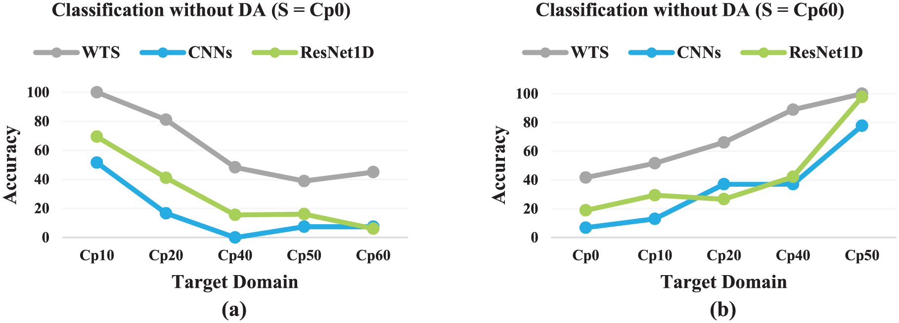
Damage detection utilising WTS, CNNs and ResNet1D without DA when (a) Cp0 and (b) Cp60 was assigned as the source domain. WTS: wavelet time scattering; CNN: convolutional neural network; DA: domain adaptation.
Figure 17 shows WTS significantly outperformed both learned backbones. With Cp0 as source, average accuracies were 73.89% (WTS), 29.67% (ResNet1D) and 30.40% (CNN). With Cp60 as source, averages were 71.89% (WTS), 42.99% (ResNet1D) and 51.33% (CNN). ResNet1D and CNN performed comparably, both exhibiting sharp accuracy drops at wider temperature gaps, while WTS maintained substantially higher performance across all transfers.
Damage detection with DA
Full SPADA was employed with the hyperparameters in Table 3, searching 1000 random configurations with maximum scale constrained to
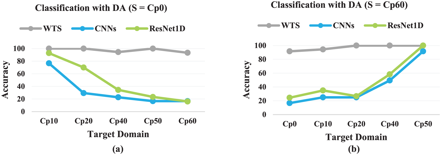
Damage detection utilising WTS, CNNs and ResNet1D with DA when (a) Cp0 and (b) Cp60 were assigned as the source domain. WTS: wavelet time scattering; CNN: convolutional neural network; DA: domain adaptation.
Figure 18 shows DA stage increases accuracy, with the largest gains at wider temperature gaps. With Cp0 source and Cp40 target, accuracy rose from 48.33 to 94.44%; with Cp0 source and Cp60 target, accuracy increased from 45 to 93.33%. With Cp60 source, accuracy increased from 41.67%, 51.67%, 66.11% to 91.67%, 94.44%, 100% for Cp0, Cp10, Cp20 targets, respectively. Small gaps (Cp0 source with Cp10 target) maintained 100%. Room for improvement remains at widest gaps (e.g., Cp60 source with Cp0 target: 91.67%). ResNet1D with DA improved over its without-DA baseline (averages rising from 29.67 to 47.34% with Cp0 and from 42.99 to 48.89% with Cp60), confirming that DA provides partial benefit with deeper learned features. However, these figures remained far below WTS with DA (96.11 and 95.56% for the same source settings), indicating that the structured, bounded feature-space displacements produced by WTS are substantially more amenable to prototype-based alignment than the less constrained representations learned by ResNet1D.
To determine residual misclassification patterns where accuracy was below 100%, Figure 19(a) to (d) presents confusion matrices for four settings: Cp0 as source with Cp60 as target, Cp0 as source with Cp40 as target, Cp60 as source with Cp0 as target and Cp60 as source with Cp10 as target.
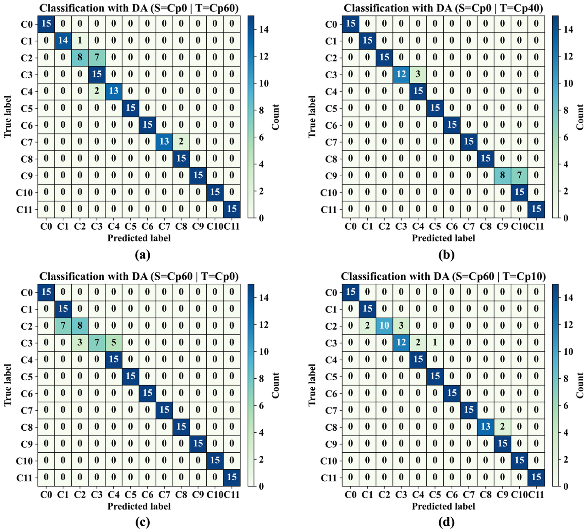
Confusion matrices for SPADA on CONCEPT for (a) source Cp0 and target Cp60, (b) source Cp0 and target Cp40, (c) source Cp60 and target Cp0 and (d) source Cp60 and target Cp10. SPADA: scattering-based prototype-aligned domain adaptation; CONCEPT: carbon–epoxy composite plate.
When Cp0 was used as source and Cp60 as target (Figure 19(a)), matrices are mostly diagonal with errors concentrated between adjacent severity classes. Largest exchanges occur between C2 and C3, with smaller leakages from C4 to C3, C1 to C2 and C7 to C8. When Cp0 was used as source and Cp40 as target (Figure 19(b)), almost all classes are correct; main deviations are C9 misclassified as C10 and minor C3 misclassified as C4. These patterns align with CONCEPT physics: Lamb waves from neighbouring severities produce highly similar dispersion and attenuation signatures, especially under larger temperature separations.
With Cp60 as source and Cp0 as target (Figure 19(c)), residual errors remain local, concentrated within C2–C4, indicating limited margins between adjacent prototypes under largest shifts. When Cp60 was used as source and Cp10 as target (Figure 19(d)), diagonals tighten further. Largest residuals occur for C2 (two samples predicted as C1, three as C3), minor errors for C3 (two samples predicted as C4, one as C5) and C8 (two samples predicted as C9); all others correct. Interpreting classes as healthy C0 and increasing delamination severities C1–C11 from incremental putty coverage, local swaps are physically plausible because adjacent severities perturb wavefields similarly between actuators and receivers. Results suggest value in class-conditional alignment or explicit pairwise margin penalties rather than global alignment alone.
Internal mechanism visualisation and interpretability analysis
To enhance transparency, SPADA logged internal states every 10 training epochs during DA: prototype vectors, instance features, pseudo-labels, entropy values and attention weights. Four t-SNE-based visualisations reveal progressive domain alignment while preserving class separability. Analysis uses two CONCEPT scenarios: Cp0 source with Cp40 target (94.44% accuracy) and Cp0 source with Cp50 target (100% accuracy). Epoch numbers on axes represent logged snapshots; multiply by 10 for actual training epochs. Entropy threshold was
Prototype trajectory evolution
Prototype trajectories were projected into 2D t-SNE space fitted on concatenated source and target prototypes across logged epochs. Trajectories sampled every 10th epoch: source prototypes as solid lines with circles, target prototypes as dashed lines with squares. Starting positions have larger filled markers with black edges; ending positions have star symbols. Figure 20(a) and (b) shows trajectories.
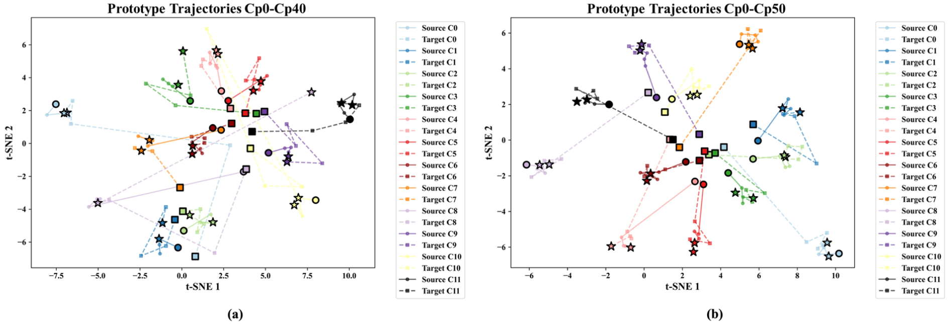
Prototype trajectory evolution through t-SNE embedding for (a) Cp0-to-Cp40 transfer and (b) Cp0-to-Cp50 transfer. t-SNE: t-distributed stochastic neighbour embedding.
For Cp0 source with Cp50 target (Figure 20(b), 100% accuracy), source and target prototypes converge to nearly coincident positions, indicating complete alignment. For Cp0 source with Cp40 target (Figure 20(a), 94.44% accuracy), class C8 prototypes diverged substantially, ending at opposite regions, likely contributing to residual errors. Classes C3 and C4 show partial convergence, while C6 and C7 achieve satisfactory alignment.
Instance-prototype cosine similarity
Heatmaps display cosine similarities between instances and prototypes at final epoch. Rows represent instances (source upper, target lower); columns represent prototypes (source left, target right). White lines delineate domains. Figure 21(a) and (b) shows similarity matrices.
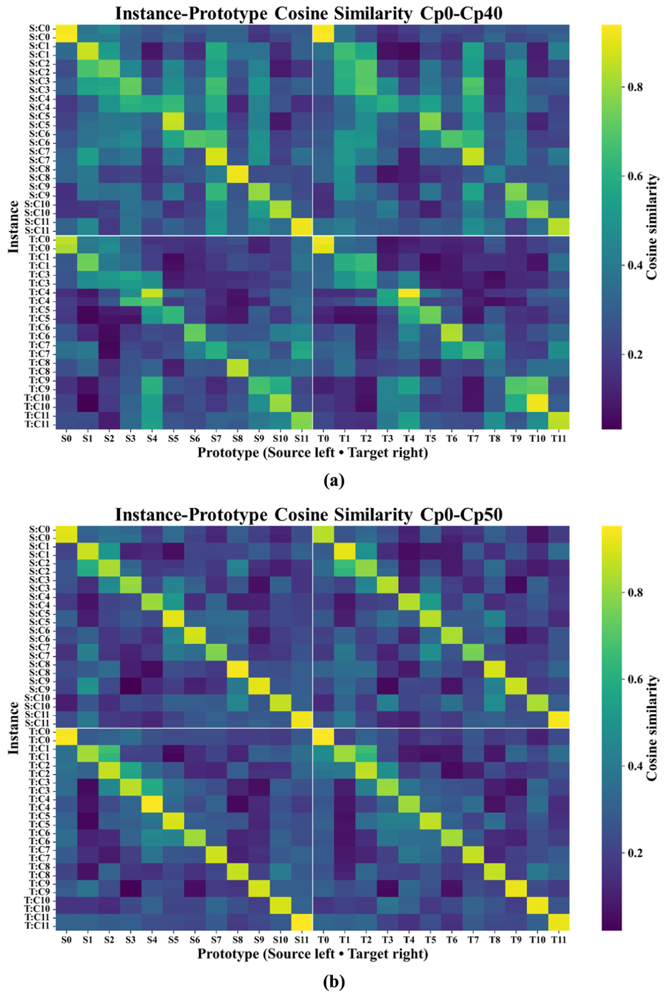
Instance-prototype cosine similarity heatmap for (a) Cp0-to-Cp40 transfer and (b) Cp0-to-Cp50 transfer.
Both graphs exhibit pronounced diagonal structures with elevated values along main diagonals, confirming instances align with corresponding class and domain prototypes. Cp0 source with Cp50 target (Figure 21(b)) demonstrates sharper diagonals with minimal off-diagonal activations (100% accuracy). Cp0 source with Cp40 target (Figure 21(a)) shows weaker diagonal intensity and moderate off-diagonal values, reflecting 5.56% error.
Prototype attention weight dynamics
Three panels track attention dynamics. Left: median source attention with IQR shading. Middle: median target attention with IQR shading. Right: pseudo-label coverage (solid line) and median target weight (dashed line). Vertical dashed line marks selected epoch. Figure 22(a) and (b) presents dynamics.
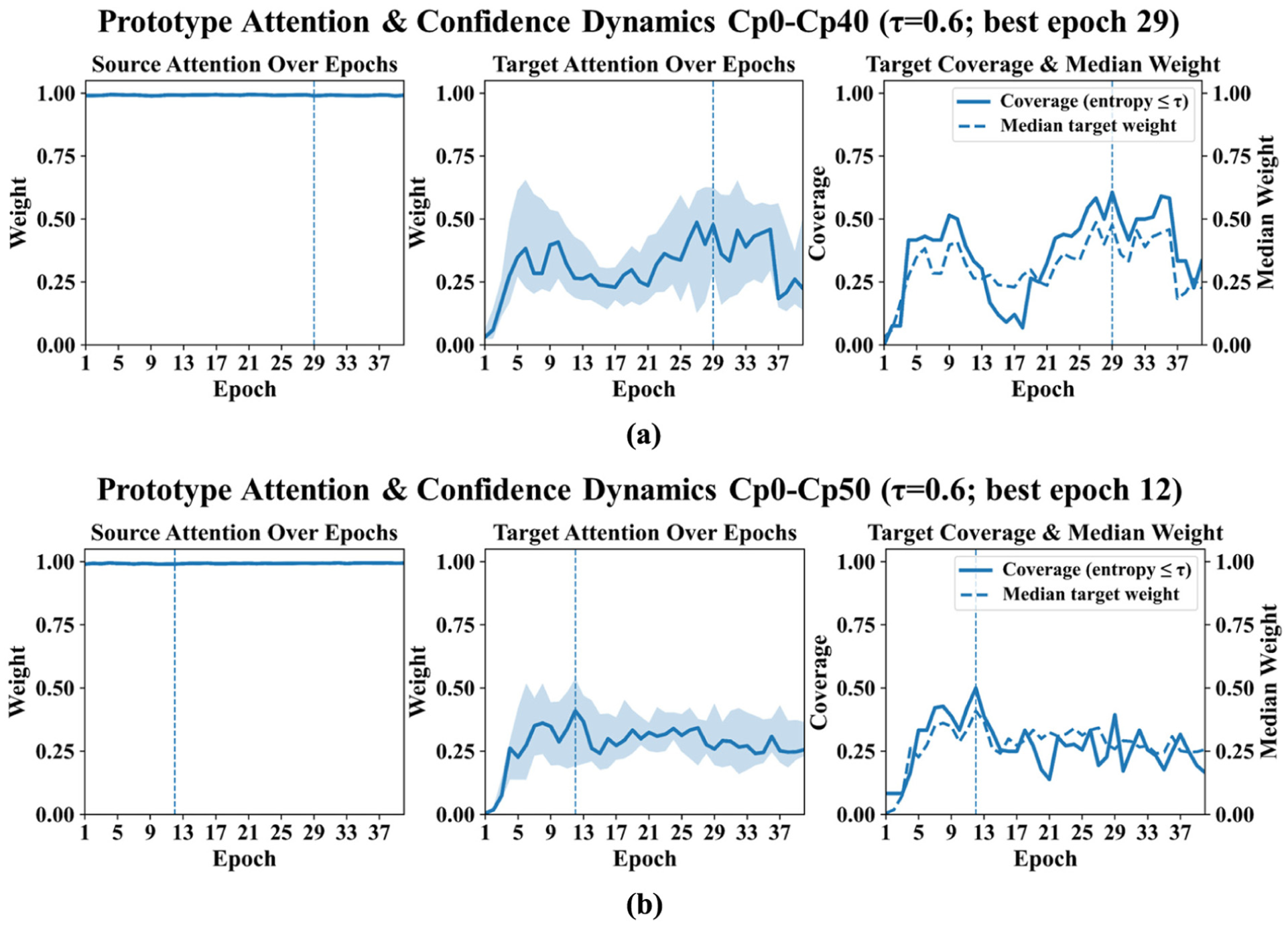
Prototype attention and confidence for (a) Cp0-to-Cp40 transfer and (b) Cp0-to-Cp50 transfer.
Source weights remain at unity. For Cp0 source with Cp50 target (Figure 22(b)), best epoch at 12, target weights stabilise around 0.3, coverage rises to 0.5 and plateaus. For Cp0 source with Cp40 target (Figure 22(a)), best epoch at 29, target weights fluctuate between 0.2 and 0.5 with wider IQR, coverage peaks near 0.6 at epoch 33 then declines. Earlier stabilisation in Cp0 source with Cp50 target corroborates superior accuracy.
Decision boundaries in feature space
Instances and prototypes projected into 2D t-SNE at best epoch. Source instances: circles; target instances: squares; source prototypes (Proto): X markers; target prototypes: filled plus symbols. Figure 23(a) and (b) shows boundaries.
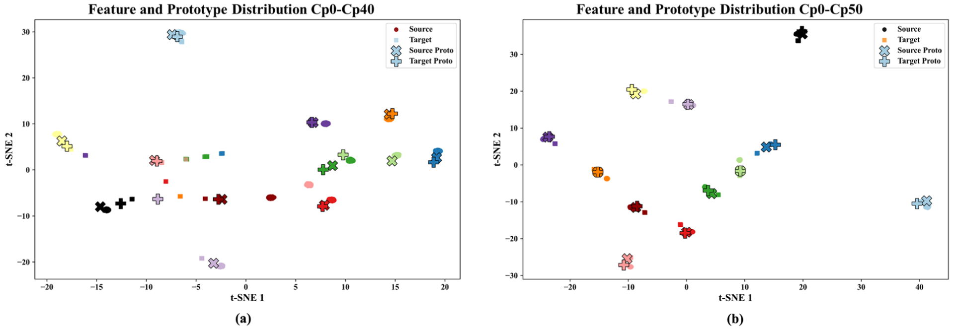
Decision boundaries in t-SNE embedding space for (a) Cp0-to-Cp40 transfer and (b) Cp0-to-Cp50 transfer. t-SNE: t-distributed stochastic neighbour embedding.
Cp0 source with Cp50 target (Figure 23(b)) shows tight, well-separated clusters by class with prototypes coincident or proximate, confirming complete convergence. Cp0 source with Cp40 target (Figure 23(a)) exhibits looser clustering with noticeable prototype gaps, visually corroborating 5.56% accuracy deficit.
Native-space quantitative metrics
To complement the t-SNE visualisations with quantitative measures computed directly in the 64-dimensional latent space, two metrics were tracked over training epochs for the Cp0 to Cp40 and Cp0 to Cp50 transfers (Figure 24). The prototype separation ratio (PSR), defined as the mean inter-class prototype Euclidean distance divided by the mean intra-class instance-to-prototype distance, quantifies how well-separated the class prototypes are relative to the dispersion of instances around them. The silhouette score, computed on instance features with class labels (true labels for source, pseudo-labels for target), provides a complementary global measure of cluster quality.
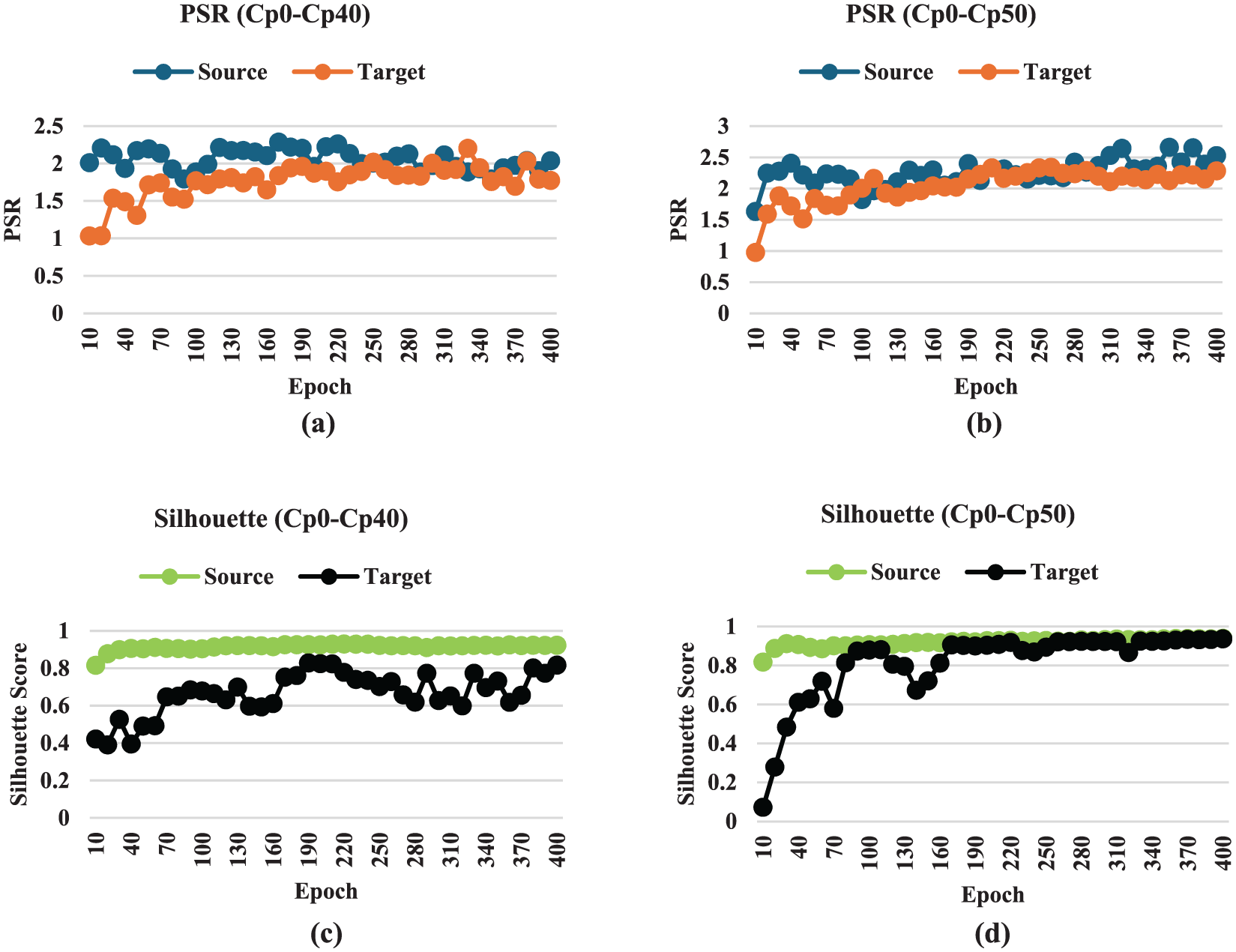
Native-space quantitative metrics over training epochs for CONCEPT: PSR for (a) Cp0-to-Cp40 transfer and (b) Cp0-to-Cp50 transfer, and silhouette score for (c) Cp0-to-Cp40 transfer and (d) Cp0-to-Cp50 transfer. CONCEPT: carbon–epoxy composite plate; PSR: prototype separation ratio.
Figure 24 represents that for both transfers, the source-domain PSR and silhouette remained high and stable throughout training (PSR approximately 2, silhouette above 0.9), confirming that source class structure was preserved during adaptation. The target-domain metrics exhibited markedly different trajectories: PSR rose from 1.03 to 1.77 (Cp40) and from 0.98 to 2.28 (Cp50), while silhouette increased from 0.42 to 0.82 (Cp40) and from 0.07 to 0.94 (Cp50). The convergence of target metrics towards source-domain values provides quantitative evidence, independent of t-SNE projection, that the adaptation mechanism progressively organises target representations into class-discriminative clusters consistent with the source-domain structure. The stronger improvement for Cp50 is consistent with its higher final classification accuracy (100 vs 94.44% for Cp40).
Comparison study
SPADA framework was evaluated against six reference methods by employing WTS for feature extraction with different UDA modules: adversarial DA with prototypes (ADA-Proto), 39 multi-domain adversarial DA with prototype attention (MADA-Proto), 40 generative adversarial network with prototype weighting (GAN-Proto), 41 central moment discrepancy (CMD), 42 correlation alignment (CORAL) 43 and neighbour refinement consistency with virtual adversarial training (NRC-VAT). 44 Experiments used augmented WTB-VibClimate and CONCEPT datasets. Challenging shifts were considered: Wp20 source with Wn15 and Wp40 targets for WTB-VibClimate; Cp0 source with Cp60 target and Cp60 source with Cp10 target for CONCEPT.
For each method, 1000 configurations were sampled without replacement from the corresponding hyperparameter ranges and evaluated across 15 independent seeds. All methods followed the same search protocol; the sole difference was the selection criterion: SPADA retained the configuration with the highest mean unsupervised A/B score, while the baselines retained the configuration with the highest mean target-domain validation accuracy. SPADA therefore operates under a more constrained selection regime, as no target labels are used at any stage.
To validate that the unsupervised A/B score provides a meaningful proxy for true target-domain performance, Spearman rank correlations were computed between the mean unsupervised score and mean target accuracy across 1000 sampled configurations (15 seeds each) for two representative CONCEPT transfers. For Cp0 to Cp10 (small temperature gap),
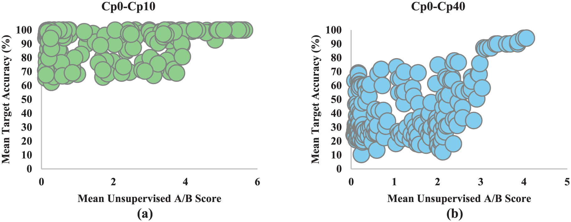
Scatter plots of mean unsupervised A/B score versus mean target accuracy for (a) Cp0-to-Cp10 transfer and (b) Cp0-to-Cp40 transfer.
Figure 26(a) to (d) shows accuracy for each source–target combination.
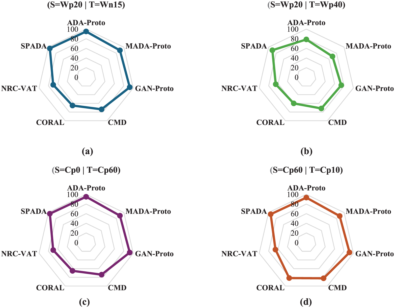
Damage detection results of UDA benchmarks against SPADA for (a) WTB-VibClimate source Wp20 and target Wn15, (b) WTB-VibClimate source Wp20 and target Wp40, (c) CONCEPT source Cp0 and target Cp60 and (d) CONCEPT source Cp60 and target Cp10. UDA: unsupervised domain adaptation; SPADA: scattering-based prototype-aligned domain adaptation; WTB-VibClimate: small-scale wind turbine blade under varying climate conditions; CONCEPT: carbon–epoxy composite plate.
Figure 26 reveals SPADA delivers the highest accuracy across all transfers, with largest advantage on Wp20 to Wp40. For WTB-VibClimate, SPADA attains 96.15% (Wp20 to Wn15), exceeding ADA-Proto by 1.06 percentage points, and 90% (Wp20 to Wp40), outperforming next best by 11.47 percentage points. Prototype-based adversarial baselines generally outperform CMD, CORAL, and NRC-VAT but trail SPADA. For CONCEPT, SPADA achieves 91.67% (Cp0 to Cp60), ahead of GAN-Proto by 1.67 percentage points, and 94.44% (Cp60 to Cp10), ahead of ADA-Proto by 1.11 percentage points. Across all four shifts, SPADA shows smallest performance spread at 6.15%, indicating both improved peak performance and stability across distinct domain shifts.
To assess how sensitive the final performance is to random seed variation in the frameworks discussed above, Table 4 reports the standard deviations (across 15 seeds) of the accuracies for SPADA, ADA-Proto, MADA-Proto, GAN-Proto, CMD, CORAL and NRC-VAT on the four representative source–target domain crosses described above.
Standard deviations of accuracy across 15 seeds for the four representative source–target crosses.
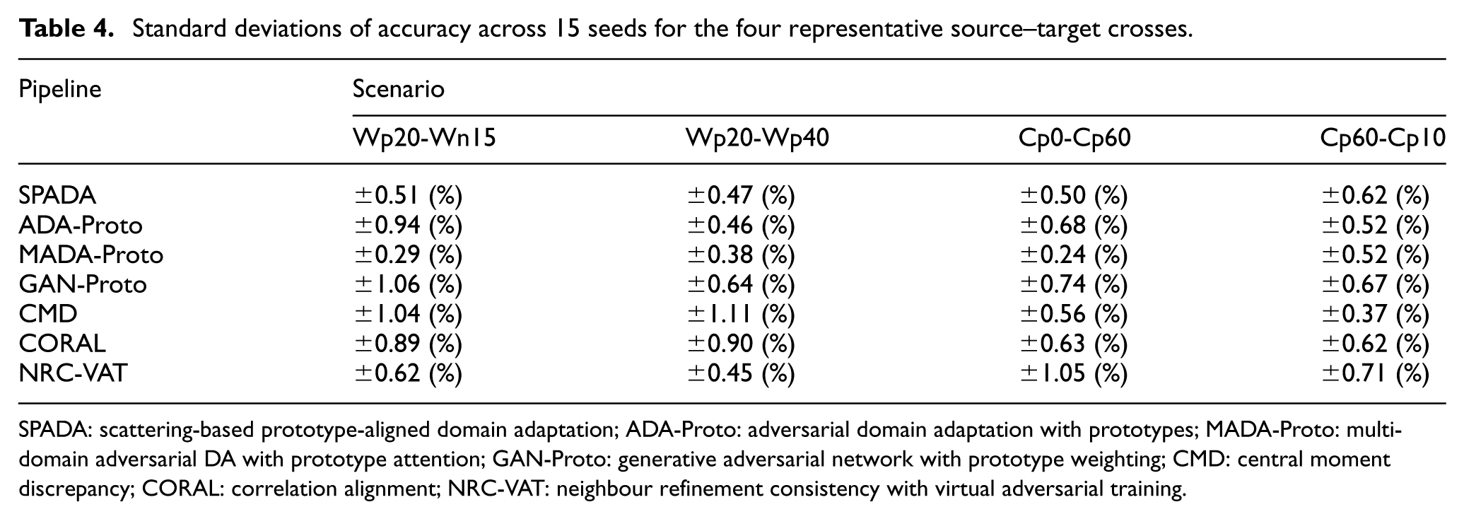
SPADA: scattering-based prototype-aligned domain adaptation; ADA-Proto: adversarial domain adaptation with prototypes; MADA-Proto: multi-domain adversarial DA with prototype attention; GAN-Proto: generative adversarial network with prototype weighting; CMD: central moment discrepancy; CORAL: correlation alignment; NRC-VAT: neighbour refinement consistency with virtual adversarial training.
Table 4 indicates that SPADA’s performance is weakly sensitive to random seed changes, with standard deviations ranging from ±0.47 to ±0.62% across the four representative transfers. This low dispersion suggests that the reported accuracies are not driven by a few favourable initialisations or stochastic training effects, but are reproducible across independent runs. In contrast, a number of baselines show noticeably higher variability in at least one transfer (e.g., CMD up to ±1.11%, GAN-Proto up to ±1.06%, NRC-VAT up to ±1.05%), indicating less stable optimisation or greater sensitivity to stochasticity under the same evaluation protocol. Consistent with this, the manuscript reports final results as means across 15 independent seeds, with all major randomness sources controlled, supporting reliable comparison between methods under identical experimental conditions.
Ablation study
To isolate the contribution of each SPADA component, three ablation variants were evaluated on the Cp0 to Cp40 transfer, using the unsupervised-selected configuration across 15 seeds. Removing adversarial alignment (
Computation efficiency
This study placed particular emphasis on the computational efficiency and practical implementation of the SPADA framework. All training, evaluation and the grid search were performed in Python 3.10 using Jupyter Notebook on a workstation running Microsoft Windows 11 Pro for Workstations (Build 26200). The experiments were executed on CPU only, using an Intel(R) Xeon(R) Gold 6248R @ 3.00 GHz with 24 cores and 48 logical processors, 192 GB of physical memory and 250 GB of virtual memory. Configurations were executed in parallel across the available cores. The core software stack comprised PyTorch 2.0.1, Scikit-learn, NumPy and Matplotlib. The wall-clock time per hyperparameter configuration (single seed, including training and unsupervised validation) was 11.88 and 16.14 s for CONCEPT and WTB-VibClimate, respectively. Each configuration was evaluated across 15 seeds, and the full grid search over 1000 sampled configurations took about 102 and 138 min for CONCEPT and WTB-VibClimate, respectively, with parallelisation across available cores. Feature extraction via WTS was cached across configurations sharing the same scattering parameters and constituted a negligible fraction of total computation. Per-sample inference latency at test time (feature extraction plus forward pass) was below 1 ms on the same hardware. From a computational standpoint, the inference stage of SPADA is compatible with online monitoring requirements on standard server-class hardware; the grid search represents an off-line training cost that would not recur during operational deployment.
Conclusion
This work addressed the challenge of deploying damage detection models under changing environmental conditions in SHM by developing an interpretable UDA framework (SPADA). The framework combines WTS for physics-guided feature extraction with prototype-based transfer learning and dedicated interpretability modules, providing clear evidence of how damage-sensitive patterns behave during environmental transitions while maintaining strong classification performance. The key findings are summarised below:
(1) Practicality: WTS is used to obtain deformation-stable representations that suppress selected environmental variations while preserving damage-related modulations in guided wave and vibration signals. These scattering coefficients are processed by a prototype-based adaptation mechanism that maintains explicit correspondence between source and target exemplars, while instance to prototype similarities and low-dimensional visualisations reveal how prototypes move in latent space, how decision regions emerge and where misclassifications tend to concentrate.
(2) Effectiveness: Validation on an experimental composite plate under temperature variation, using temperature-conditioned synthetic damaged responses generated by the Conv-CVAE, and on the WTB benchmark dataset of vibration signals, demonstrated successful knowledge transfer without requiring labelled target data. Prototype tracking showed that damage classes largely preserved their structural characteristics during temperature-induced transfer, with trajectories and confusion patterns following expected trends. The interpretability diagnostics indicated that performance degradations mainly occurred between neighbouring damage severities and that the class structure of source and target data remained well separated, suggesting that adaptation preserved damage-sensitive information rather than collapsing classes due to environmental effects. These findings are drawn from two controlled laboratory benchmarks, one of which (CONCEPT) employs synthetic damaged signals at non-baseline temperatures generated by the Conv-CVAE. Accordingly, the robustness claims for CONCEPT transfers should be interpreted within the context of this constructed evaluation setting, while the WTB-VibClimate results provide direct experimental support across real temperature conditions.
(3) Limitations and future work: Key limitations warrant acknowledgement. The framework has been examined exclusively under temperature variations and has not yet been tested for other EOVs. The current formulation addresses classification rather than novelty detection, and the interpretability analysis relies on expert inspection rather than quantitative metrics of physical plausibility. The interpretability modules enhance diagnostic transparency but do not provide formal guarantees of physical correctness; they are designed as inspection instruments that support expert judgement rather than as certification mechanisms. Both case studies employ relatively simple structural geometries with regularly spaced sensors under controlled laboratory conditions. In more complex configurations, such as stiffened panels or curved shells, multipath reflections and mode conversions at geometric discontinuities would increase feature variability beyond temperature effects alone. While the WTS stability bound remains valid regardless of signal complexity, the prototype-based alignment may require greater adaptation capacity to accommodate richer feature distributions. Sparse or irregular sensor layouts would further reduce the discriminability of scattering coefficients for closely spaced damage classes, and the Conv-CVAE fixed-offset synthesis strategy would be less likely to generalise where damage-induced waveform changes depend strongly on actuator-damage-sensor geometry. Future work will extend the framework to multi-source DA, integrate physics-based constraints derived from wave propagation models, and progress from classification to damage localisation and severity estimation within digital twin workflows. Addressing more complex structural geometries, irregular sensor configurations and additional environmental variabilities constitutes a further priority for investigation.
Footnotes
Notation
ADA-Proto adversarial domain adaptation with prototypes
CC cross correlation
CMD central moment discrepancy
CNNs convolutional neural networks
CONCEPT carbon-epoxy composite plate
CORAL correlation alignment
CWI coda wave interferometry
DA domain adaptation
DTW dynamic time warping
EMA exponential moving average
EOVs environmental and operational variabilities
FRFs frequency-response functions
GAN-Proto generative adversarial network with prototype weighting
MADA-Proto multi-domain adversarial domain adaptation with prototype attention
NRC-VAT neighbour refinement consistency with virtual adversarial training
PCA principal component analysis
PZT lead zirconate titanate
SHM structural health monitoring
PSR prototype separation ratio
t-SNE t-distributed stochastic neighbour embedding
UDA unsupervised domain adaptation
WTB-VibClimate small-scale wind turbine blade under varying climate conditions
WTS wavelet time scattering
Declaration of conflicting interests
The authors declared no potential conflicts of interest with respect to the research, authorship, and/or publication of this article.
Funding
The authors disclosed receipt of the following financial support for the research, authorship, and/or publication of this article: This research study was carried out in the framework of the project “TU-LEARN—sTrUctural Life Extension enhAnced by aRtificial iNtelligence,” funded by Unione europea—Next Generation EU, as part of Prin 2022 PNRR—D.D. n. 1409 del 14-09-2022 program.
Data availability Statement
The data that support the findings of this study are available upon reasonable request from the corresponding author.