
Abstract
In structural health monitoring (SHM), the scarcity of labeled data representing different structural states and structural configurations remains a key challenge for developing robust and generalizable deep learning models. Building upon a reported attention-enhanced star generative adversarial network with gradient penalty (AT-StarGAN-GP), this study examines its application to generating synthetic structural vibration signals that reflect both cross-structure domain differences and multiple localized structural state scenarios. The framework supports conditional translation across domains, learning from acceleration responses measured on a source structure to generate synthetic responses for a target structure under structural state conditions. The architecture integrates multi-type attention mechanisms, including self-attention, channel-attention, and spatial-attention, and evaluates four conditioning strategies: concatenation (Concat), feature-wise linear modulation (FiLM), adaptive instance normalization (AdaIN), and conditional instance normalization (CIN). A dual-conditional formulation based on joint location and structural state level is employed. The framework is evaluated using two small-scale physical bridge models, each instrumented at six joint locations, with structural state variations simulated at selected joints using three mass levels (no mass, low mass, and high mass). Evaluation across modal, temporal, distributional, and spectral metrics shows that CIN provides improved performance, achieving a modal assurance criterion of 0.894, frequency response assurance criterion of 0.872, the lowest distributional discrepancy (maximum mean discrepancy 0.0006), and an 86% pass rate in Kolmogorov–Smirnov tests. Attention mechanisms improve localization accuracy by 34.35% and reduce entropy by 6.98%, while self-attention reduces cross-domain Kullback-Leibler (KL) divergence by 24.5%. The AdaIN variant shows more consistent behavior under unseen-domain scenarios (MAC 0.8207–0.8405). All evaluated configurations retain over 94% of baseline performance under 25% noise. Five-fold cross-validation confirms training stability, and Friedman–Nemenyi testing indicates statistically significant separation from weaker baselines, although differences relative to mid-tier methods remain limited in some comparisons. Overall, the results indicate that the extended AT-StarGAN-GP framework can generate structurally consistent synthetic vibration responses across different structures and state conditions under controlled laboratory settings.
Keywords
Introduction
Structural health monitoring (SHM) has developed as a significant discipline over several decades, with foundational contributions in modal analysis emerging in the 1980s and the implementation of permanent monitoring systems on civil infrastructure beginning in the 1990s and early 2000s. Comprehensive assessments1,2 and seminal texts 3 on modal testing 4 and on SHM principles provided the theoretical and practical foundations of the field. SHM is a vital discipline within civil engineering, aiming to ensure the safety and longevity of infrastructure through continuous observation and assessment. By analyzing measurements from sensors placed on structures,5,6 SHM systems can detect and localize damage at an early stage, thereby minimizing maintenance costs and preventing catastrophic failures. Among various sensing approaches,7,8 vibration-based SHM stands out due to its ability to capture the dynamic behavior of a structure under ambient or operational loading. Changes in modal parameters such as natural frequencies, 9 mode shapes, and damping ratios often indicate the presence and severity of structural damage.10,11 Modern SHM implementations heavily rely on accelerometers and similar vibration sensors to record high-resolution time-series data, forming the basis for data-driven damage detection frameworks. Recent work has also explored the use of single-output operational modal analysis with smartphone accelerometers placed on bridge decks and moving vehicles, showing that changes in natural frequencies from baseline conditions may indicate loss of stiffness and potential structural damage. Environmental and operational uncertainties should be taken into account for an efficient diagnostics procedure, and the level of mobility (LoM) framework has been adopted to clarify how smartphone sensing interacts with the structure. 12 In their study, LoM1 (Stationary Invasive) refers to a smartphone placed directly on the bridge deck, while LoM3 (Vehicular/Drive-By) refers to a smartphone mounted on a moving scooter. These two mobility levels were used to demonstrate their comparative and complementary effectiveness in identifying bridge modal characteristics.
Despite the technological progress in sensor development and data acquisition systems, SHM faces several fundamental challenges. A key issue is the scarcity of labeled damage data, which hinders the training and validation of supervised learning algorithms.13,14 Most real-world datasets contain abundant information for undamaged or baseline conditions, but limited data for damaged states, especially for multiple or progressive damage scenarios. This imbalance leads to biased models with limited generalizability. Structural vibration signals are influenced by environmental and operational variability, 15 such as temperature fluctuations or loading changes, introducing noise and uncertainty. Wireless sensor networks, which are often used in long-term monitoring, are also prone to data loss, 16 creating gaps in time-series recordings. The accumulation of continuous monitoring data over time generates large-scale datasets, imposing significant demands on storage, processing, and interpretation. 17 To address these data-related limitations, researchers have turned to deep learning models, which offer powerful tools for feature extraction and classification from raw vibration signals. Convolutional neural networks (CNNs) have shown particular promise for extracting local features from acceleration time-series, capturing signal patterns associated with specific damage scenarios. 18 One-dimensional (1D) CNNs can effectively extract damage-sensitive features from raw sensor data and achieve real-time damage detection. However, CNNs are constrained by their limited receptive fields and may fail to capture long-range temporal dependencies. Recurrent neural networks (RNNs), especially long short-term memory (LSTM) networks, have been applied to overcome this shortcoming.19,20 These architectures are designed to model sequential data, capturing long-term dependencies and trends in vibration signals. Nevertheless, standalone LSTMs can underperform in extracting detailed local features and suffer from vanishing or exploding gradients on long sequences. 21 Hybrid architectures that combine CNNs for spatial encoding and LSTMs for temporal modeling have demonstrated improved accuracy by leveraging both local and global characteristics of structural response data.
Transformer-based models with attention mechanisms have been introduced to address the trade-offs between spatial and temporal modeling.21,22 Transformers use self-attention to learn global relationships across sequences, enabling them to capture complex interactions in structural vibration data. A Conformer network that integrates convolution and attention modules has been proposed, achieving enhanced robustness against noise and improved accuracy. 23 Similarly, a novel cross-fidelity deep learning framework has been proposed that integrates seismic ground motions with low-fidelity structural responses to predict high-fidelity seismic responses in steel frame buildings. 24 The hybrid model combines CNN, LSTM, and Transformer architectures to capture complex time-frequency-magnitude dependencies in seismic data. Experimental results on California steel frame buildings demonstrate that this approach outperforms other single- and dual-input models, enhancing the accuracy and robustness of dynamic response predictions. Many of these models exhibit limited generalization when applied to new structures or untrained conditions. CNNs trained on one structure performed poorly on others due to domain shifts, highlighting the need for transfer learning and domain adaptation strategies. 25 To mitigate this data scarcity, deep generative models (DGMs) have been introduced to synthesize realistic structural response data. Recent comprehensive meta-analyses have systematically examined the application of generative artificial intelligence and data augmentation techniques for prognostics and health management (PHM) across various engineering domains. A detailed taxonomy of data augmentation and generation techniques for PHM has been provided, 26 categorizing approaches into data-based randomized methods, mechanism-based domain-specific techniques, and feature-based generative models. The critical role of generative adversarial networks (GANs), variational autoencoders (VAEs), and diffusion models in addressing data scarcity challenges has been highlighted. An extensive review of DGMs in condition monitoring and SHM has been conducted, examining state-of-the-art deep autoregressive models, VAEs, GANs, diffusion-based models, and large language models across rotating machinery, aircraft structures, wind turbines, and civil infrastructure applications. 27 While GAN-based approaches currently dominate data generation tasks, diffusion-based models and large language models remain in early stages of industrial practice, presenting significant opportunities for future development.
Building on these comprehensive reviews, it has been demonstrated 28 that GANs have gained significant popularity. 1D GANs are capable of generating synthetic acceleration signals that closely match real data, improving classifier performance under data-limited conditions. These models have been employed not only for data generation but also for data augmentation, domain translation, and anomaly detection. The application of these models has been further extended. Conditional GANs and CycleGANs have additionally enhanced this capability by learning mappings between undamaged and damaged domains, enabling the synthesis of paired data from single-domain observations.29,30 Transformer-based GANs, such as the Time-Series Wasserstein GAN, 31 combined the benefits of attention mechanisms with generative modeling, producing realistic synthetic sequences at reduced computational costs. The potential of VAEs and diffusion models for SHM data augmentation has been explored, demonstrating their ability to capture probabilistic latent representations and generate high-fidelity variations of structural responses.32,33 One of the most flexible generative models, StarGAN, was introduced 34 for image-to-image translation across multiple domains using a single generator-discriminator framework and was extended to StarGAN v2. These models have been successfully applied in various domains, including face synthesis, 35 voice conversion,36,37 and electroencephalogram (EEG) signal generation. 38 By using domain labels or style codes to condition the generation process, a single model is enabled to learn mappings among multiple target classes. While StarGAN has demonstrated strong performance in other fields, its potential in SHM, particularly for multi-scenario vibration signal generation, remains largely unexplored. A further gap in SHM research has been identified, namely the lack of studies addressing multiple concurrent damage scenarios.39,40 Most existing datasets and models focus on single-damage conditions, whereas real-world structures often experience progressive or multi-site failures. Few studies have attempted to model such complexity. A rare multi-damage Lamb-wave dataset for composite materials has been developed; however, comprehensive, scalable, and labeled datasets for multi-damage vibration scenarios are virtually nonexistent. 41
Moreover, generative modeling in SHM has primarily focused on single-damage augmentation, leaving multi-damage synthesis largely unexplored. To address this gap, AT-StarGAN-GP, an attention-enhanced generative adversarial framework designed for structural vibration data and previously applied to same-structure signal translation, is further examined in this study. 42 The framework incorporates dual attention mechanisms to represent global temporal dependencies and local signal interactions, while a Wasserstein loss with GP is used to support stable training. The ability of the model to reproduce modal characteristics, including natural frequencies and damping ratios, is evaluated through comparisons between synthetic and measured signals. In the present study, the framework is applied to the simulation and classification of localized, multi-level structural states at individual joints. Multiple levels of additional mass are introduced at selected locations within the structure as a controlled representation of structural state changes. Signal generation and discrimination are considered for three state levels per joint: no mass, low-level mass, and high-level mass. Training is conducted using data from a source structure, and evaluation is performed on a distinct target structure to examine cross-structure domain translation.
Relative to the previously reported AT-StarGAN-GP framework for same-structure vibration signal translation, 42 the following aspects are considered in this study:
Cross-structure domain translation: The framework is applied to cross-structure domain translation, with training performed on a source structure and evaluation conducted on a distinct target structure.
Structural state conditioning: Structural state information is incorporated into the conditioning scheme, enabling signal generation corresponding to multiple localized state scenarios defined by different mass levels.
Dual-conditional learning: A joint conditioning approach based on sensor location and structural state level is used to represent spatial variability and state severity within the signal generation process.
Multi-level structural state simulation: Signal generation is extended from healthy-state conditions to three structural state levels (no mass, low mass, and high mass) at multiple joints.
The following section describes the AT-StarGAN-GP framework, modified as required to address the cross-structure domain translation and structural state conditioning considered in this study, including its architectural components, loss formulation, and training procedure, along with the experimental setup used for evaluation.
Methodology
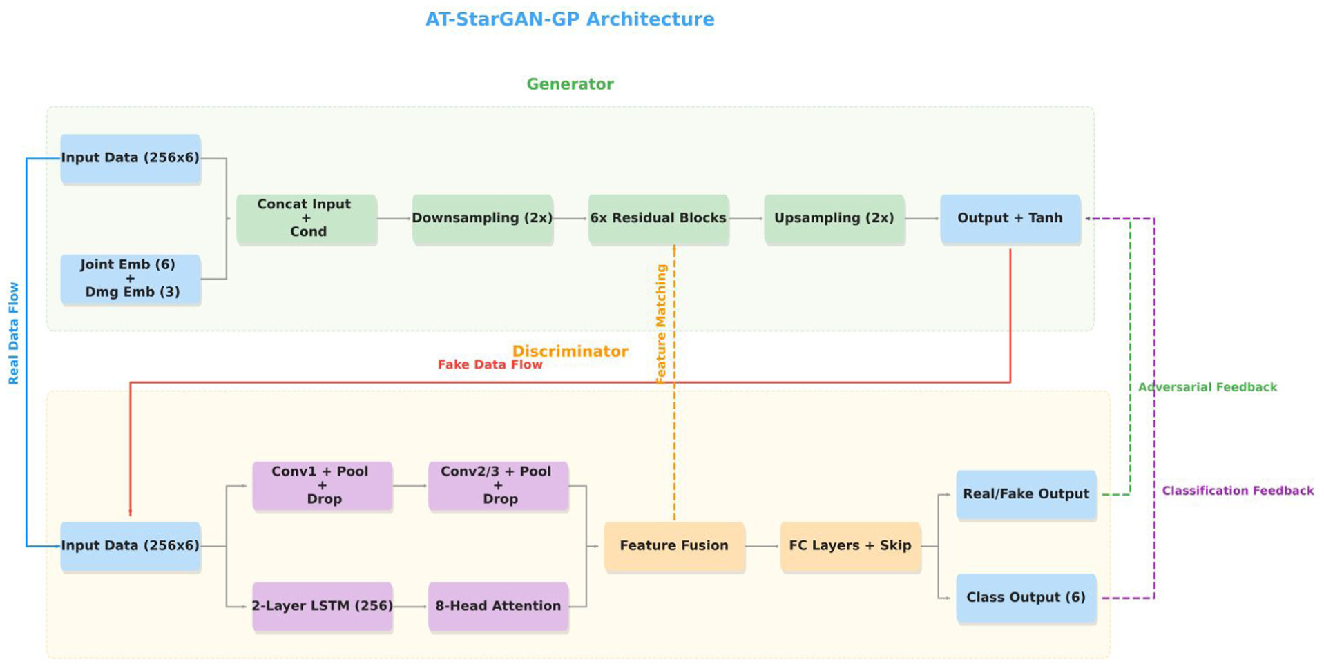
This paper presents the AT-StarGAN-GP framework, designed to perform multi-scenario structural state generation, cross-structure domain translation, and SHM-oriented conditional signal synthesis. The architecture integrates multi-conditional inputs, enabling simultaneous control over joint location, structural state, and structural domain while preserving the dynamic characteristics of each system. Figure 1 provides an overview of the complete AT-StarGAN-GP pipeline, illustrating how these conditioning mechanisms and the adversarial training strategy operate throughout the model.
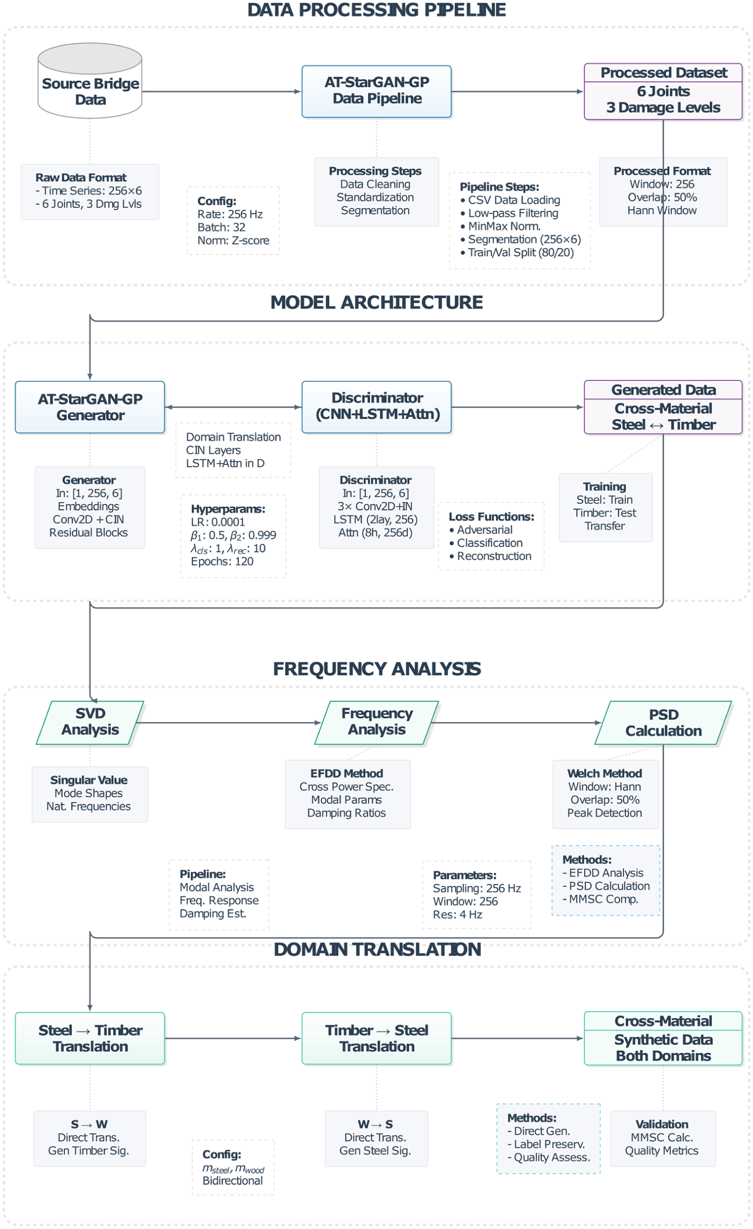
Overall workflow of the proposed AT-StarGAN-GP model, synthetic data generation model, and modal analysis. AT-StarGAN-GP: attention-enhanced star generative adversarial network with gradient penalty.
Experimental dataset involves accelerometer measurements taken from two different small-scale bridge models: a steel bridge (used as the target structure) and a timber bridge (used as the source structure), shown in Figure 2(a) and (b), respectively. Both bridges were instrumented identically with six accelerometers placed at six joint locations, following the same measurement protocols within their respective structural domains. Each joint was subjected to one of three predefined mass conditions: level 0 (baseline state with no added mass), level 1 (low added mass), and level 2 (high added mass). These conditions were created using a controlled added-mass technique involving steel plates, four plates (4 kg) for level 1 and eight plates (8 kg) for level 2. The plates were strategically placed at three joint regions between accelerometer pairs 1–5, 3–6, and 4–7, as illustrated in Figure 2.
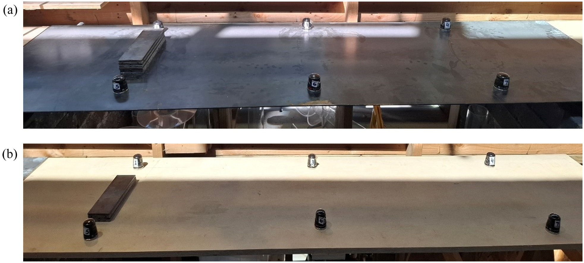
Bridge models: (a) target structure—steel bridge (higher mass at position 1) and (b) source structure—timber bridge (lower mass at position 1), both instrumented with six accelerometers.
The dataset was carefully designed to balance comprehensive structural coverage with practical experimental constraints. In both structural domains, the same protocol was followed: a reference state with no added mass, combined with six conditions created by adding identical masses to each of three positions. This symmetric distribution of mass enables a systematic study of localized structural states in an experimentally tractable setting. In this case, the ability of AT-StarGAN-GP to translate domain-specific structural responses produced using different structures is tested through this parallel setting, thus offering a strictly aligned framework to deduce cross-domain correlations.
The sampling frequency was set at 128 Hz to ensure sufficient temporal resolution for capturing the fundamental vibrational modes and their harmonics, which are critical for detecting mass-induced structural changes. This frequency supports accurate assessment of both global and local dynamics in small-scale structures. The experimental time-series captures the full temporal response of each structure under controlled excitation, with synchronized acceleration signals recorded simultaneously by six spatially distributed sensors. This multi-channel setup provides the deep learning model with complex mode shapes and spatial correlations necessary to distinguish between different structural states and domains.
The raw data were preprocessed before training the neural networks to retain important structural characteristics and enable efficient computation. Acceleration signals from each channel were separated and rearranged according to their physical layout, maintaining the crucial spatial-temporal correlations needed to identify unique patterns associated with different mass distributions. To address the requirements of modal parameter identification under temporal segmentation, a Hann window with 50% overlap was applied. A window size of 256 samples was selected as an optimal trade-off between temporal resolution and computational cost, while the Hann window helped reduce spectral leakage. Overlapping windows allowed for capturing transient phenomena without sacrificing statistical independence between successive segments, maximizing information extraction and the diversity of the training dataset.
Normalization was performed using a MinMaxScaler to independently scale each accelerometer channel to the range [−1, 1], mitigating intersensor variability in response and installation specifics. This ensured that only the relative amplitude patterns, critical for capturing spatial information and identifying mode shape changes due to added mass, were retained. The same scaling parameters were applied across training, validation, and testing to maintain model stability.
To facilitate training of the AT-StarGAN-GP model, a systematic labeling system was implemented. Experimental joints were indexed from 0 to 5, preserving joint identity while enabling efficient categorical embedding. Structural states were assigned ordinal labels: 0 for the no-mass baseline, 1 for the lower mass level, and 2 for the higher mass level. This ordered labeling reflects realistic progression of structural states and enables the model to learn smooth transitions between them, thereby enhancing the fidelity of generated synthetic data.
The generator adopts an encoder–decoder architecture with CIN to enable multi-domain translation. The input to the generator is an acceleration tensor of size
The encoder begins with a convolutional layer containing 64 filters (3 × 3 kernel, stride 1, padding 1), followed by CIN and Rectified Linear Unit (ReLU) activation. Two downsampling blocks then increase the channel depth to 128 and 256 via strided convolutions, each followed by CIN and ReLU. The bottleneck consists of six residual blocks operating at 256 channels, where CIN incorporates both conditioning signals through learnable affine transformations. The decoder mirrors the encoder using transposed convolutions to upsample features back to the original resolution. A final 7 × 7 convolution with tanh activation produces the output signal constrained to [−1, 1], with bilinear interpolation ensuring dimensional consistency.
For a feature map with C channels, CIN generates scaling and shifting parameters from both mass-type and position embeddings. Each embedding produces 2C parameters, and the final normalization is computed as the average of the two conditioning effects. This formulation balances the influence of structural state and joint location while preserving instance-specific characteristics.
The discriminator uses a combined CNN-LSTM architecture with a multi-head attention module to perform real/fake discrimination and conditional classification. The CNN branch extracts spatial–temporal features using three convolutional blocks with increasing channel sizes (64, 128, and 256), while keeping the accelerometer channel dimension unchanged. In parallel, a two-layer bidirectional LSTM with 256 hidden units processes the raw time-series data to capture longer-term temporal patterns.
Self-attention with eight heads is applied to the LSTM output to highlight time segments that contribute most to the classification tasks. The resulting attention-based features are combined with the flattened CNN features and passed through shared fully connected layers. The network then produces three outputs corresponding to real/fake discrimination, mass-level classification, and position classification.
The AT-StarGAN-GP model is trained using a combination of adversarial, classification, cycle-consistency, reconstruction, and diversity losses within a Wasserstein GAN (WGAN)-GP setting. The GP term is used to improve training stability, while the cycle-consistency and reconstruction losses help maintain similarity between original and translated signals. The diversity loss is included to reduce the risk of mode collapse by promoting variation among generated samples.
Training is carried out using an alternating update scheme, where the discriminator and generator are each updated once per iteration using the Adam optimizer (learning rate 0.0002, β1 = 0.5, β2 = 0.999). Gradient clipping and adaptive weighting of loss terms are applied to support stable training. Mode collapse is monitored using within-class and between-class diversity measures, and when collapse indicators exceed predefined thresholds, noise injection and loss reweighting are applied. Overall, this implementation allows AT-StarGAN-GP to learn mappings between structural domains while maintaining key signal characteristics through explicit conditioning and controlled training procedures. The framework is intended to generate synthetic vibration signals that are consistent with the measured data and suitable for SHM-related studies.
Problem formulation
Conditional representation and problem setup
Multi-conditional generation allows the model to control multiple aspects of structural configuration simultaneously. By encoding joint location and mass state as one-hot vectors, the model creates separate condition spaces that can be adjusted independently while jointly influencing the generated data. This conditioning approach captures the interaction between added mass location and magnitude and provides control over the characteristics of the synthetic outputs.
The conditional information encoding process involves a systematic procedure for converting discrete, categorical data into continuous vectors that can guide the generation process. First, the conditioning variables are transformed to one-hot encodings, creating mutually exclusive categorical representations where each joint location and structural state is represented by a unique vector with only one active element that identifies the chosen state. This sparse representation preserves the categorical nature of the input and provides a standardized format for subsequent processing steps. Mathematically, for each sample, the joint location


The transformation through learned embedding layers (e) allows the model to represent categorical conditioning information as continuous vectors that can be optimized during training. Unlike fixed encodings that impose predetermined relationships between categories, the learned embeddings allow the model to adaptively determine the most effective representation space for capturing the relationships between different joint locations and structural states. The embedding dimension of 8 provides sufficient representational capacity to encode complex relationships while maintaining computational efficiency and avoiding overfitting in the embedding space. These one-hot vectors are transformed into dense embeddings through learned embedding layers:


where E represents the embedding dimension.
The Concat of joint and structural state embeddings creates a unified condition vector (c) that captures the combined influence of both factors on structural behavior. This approach recognizes that structural state effects are not simply additive across location and state dimensions, but rather exhibit complex interaction patterns that require joint representation. The combined embedding space allows the model to represent relationships where the same structural state can exhibit different behaviors depending on joint location, influenced by local stiffness, boundary conditions, and load transfer. The joint and structural state embeddings are concatenated to form a single condition vector:

The spatial broadcasting mechanism integrates the conditioning information with spatially structured input data by expanding the condition vector to match the spatial dimensions of the input signal. This makes the conditioning information available at every spatial location during processing. As a result, different regions of the signal can be influenced based on their relevance to the specified joint and structural state. The combined embedding is then spatially broadcast to match the input signal dimensions:

where H= 256 (time steps) and W= 6 (accelerometer channels). The broadcasted condition tensor is concatenated with the input signal along the channel dimension:

where
The generator network Figure 3 receives three primary inputs: the segmented acceleration matrix (256 × 6), one-hot encoded joint labels (six dimensions), and one-hot encoded structural state labels (three dimensions). These condition vectors are injected throughout the generator via CIN layers, enabling the network to generate structurally consistent outputs specific to target joint and structural state configurations.
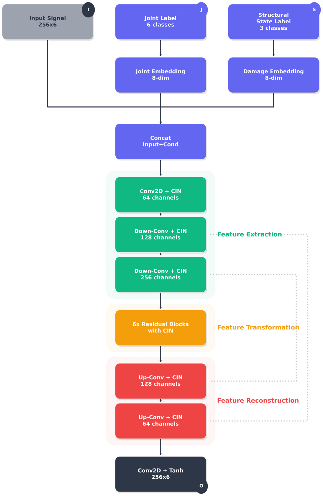
Detailed generator architecture of the proposed AT-StarGAN-GP model. AT-StarGAN-GP: attention-enhanced star generative adversarial network with gradient penalty.
This dual-conditioning formulation separates the effects of joint location and structural state, which influence the vibration response through different mechanisms. Joint labels mainly affect spatial characteristics such as mode shape expression, local stiffness variation, and sensor-dependent sensitivity. Structural state labels, representing mass changes, influence temporal and spectral properties including modal frequencies, damping ratios, and energy distribution. By encoding these factors separately and allowing the generator to merge them in its latent layers, the model can learn both their individual effects and their interactions. This design helps maintain distinctions among structural states in the embedding space, reduces the risk of merging different scenarios into similar feature patterns, and supports the preservation of temporal coherence and mode-dependent spectral content during translation.
Conditional injection and generator architecture
The generator incorporates joint location and structural state information through conditioning mechanisms that modulate feature transformations throughout the network. Three conditioning strategies are considered: Concat, FiLM, and CIN.
Concat provides the most direct approach, where the combined joint–state embedding is spatially broadcast and appended to the input or intermediate feature maps. This introduces the conditioning information into the model but does not modify the distribution of latent activations.

FiLM extends this by generating feature-wise affine transformation parameters from the conditioning embedding and applying them directly to the activations:

allowing the conditioning variables to influence the scaling and shifting of internal representations, providing more adaptive control than simple Concat.
AdaIN further increases flexibility by normalizing each feature channel and then imposing conditioning-dependent target statistics. For a feature map F, instance statistics are computed as:
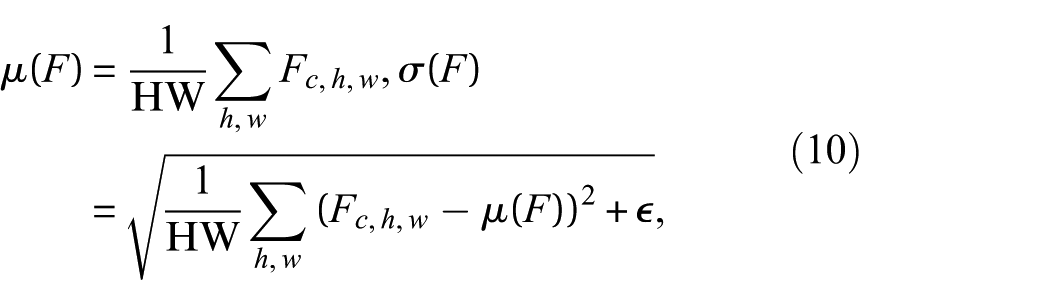
and AdaIN is applied as:
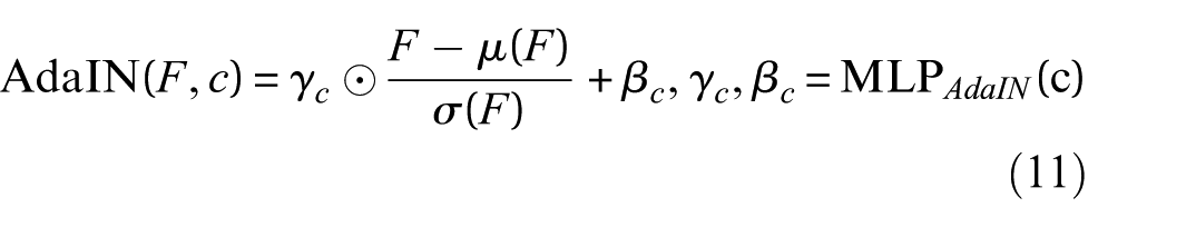
The proposed model adopts CIN as the primary conditioning mechanism. CIN modulates feature maps at multiple layers using parameters determined from the conditioning vector, enabling the generator to effectively capture the physical impact of joint and structural state variations. For each feature map
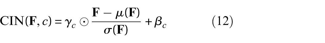
where

By adjusting normalized activations, CIN provides fine-grained channel control and allows the generator to respond to changes in joint location and structural (mass) state. This approach supports more accurate modeling of structural-frequency content and sensor-level variations than Concat or FiLM.
To improve modeling of mass-sensitive and location-sensitive global dependencies, a self-attention block is inserted at the bottleneck of the generator, after the last encoder layer and before the decoder. Given the bottleneck representation H, query, key, and value projections are computed, and attention weights are:
with the refined representation obtained through

This placement enables the generator to capture global interactions at the lowest spatial resolution with minimal additional cost.
The discriminator includes an explicit self-attention mechanism. After temporal features are extracted by the LSTM layers, an eight-head self-attention module computes relationships between temporal positions in the vibration sequence. Given the sequence representation H, query, key, and value projections are computed in the same manner as above. This attention module allows the discriminator to focus on temporally informative regions such as resonance buildup, transient peaks, or changes in damping behavior. These regions contain information that helps distinguish real from generated signals and supports accurate joint and structural state classification.
The overall generator follows an encoder–decoder structure with skip connections, illustrated in Figure 3. The encoder consists of downsampling blocks that increase channel depth from 64 to 128 and then to 256 while reducing spatial resolution. The bottleneck comprises six residual blocks equipped with CIN, enabling the model to apply conditioning-dependent transformations while retaining stable gradient flow. The decoder mirrors the encoder through upsampling layers and skip connections, restoring temporal resolution and preserving fine-grained signal details. This architecture supports accurate reconstruction of vibration responses and provides a flexible framework for conditioning-based translation across joint locations and structural states.
Discriminator and domain translation framework
The discriminator is designed to provide comprehensive feedback for both source discrimination and conditional consistency. It processes structural vibration signals through two parallel computational paths that extract complementary spatial and temporal features, as illustrated in Figure 4. The first path is a convolutional stream that progressively increases channel depth across three layers, capturing local spatial patterns and joint-dependent structural characteristics. The second path is a temporal analysis stream composed of LSTM layers combined with multi-head self-attention, enabling the network to model long-range temporal dependencies and frequency-related variations that are influenced by changes in mass or joint location. The outputs of these two paths are fused into a unified representation that feeds two dedicated prediction heads. One head estimates the probability that an input signal is real or generated, and the other performs joint and structural state classification to ensure that the generator produces signals consistent with the specified conditioning.
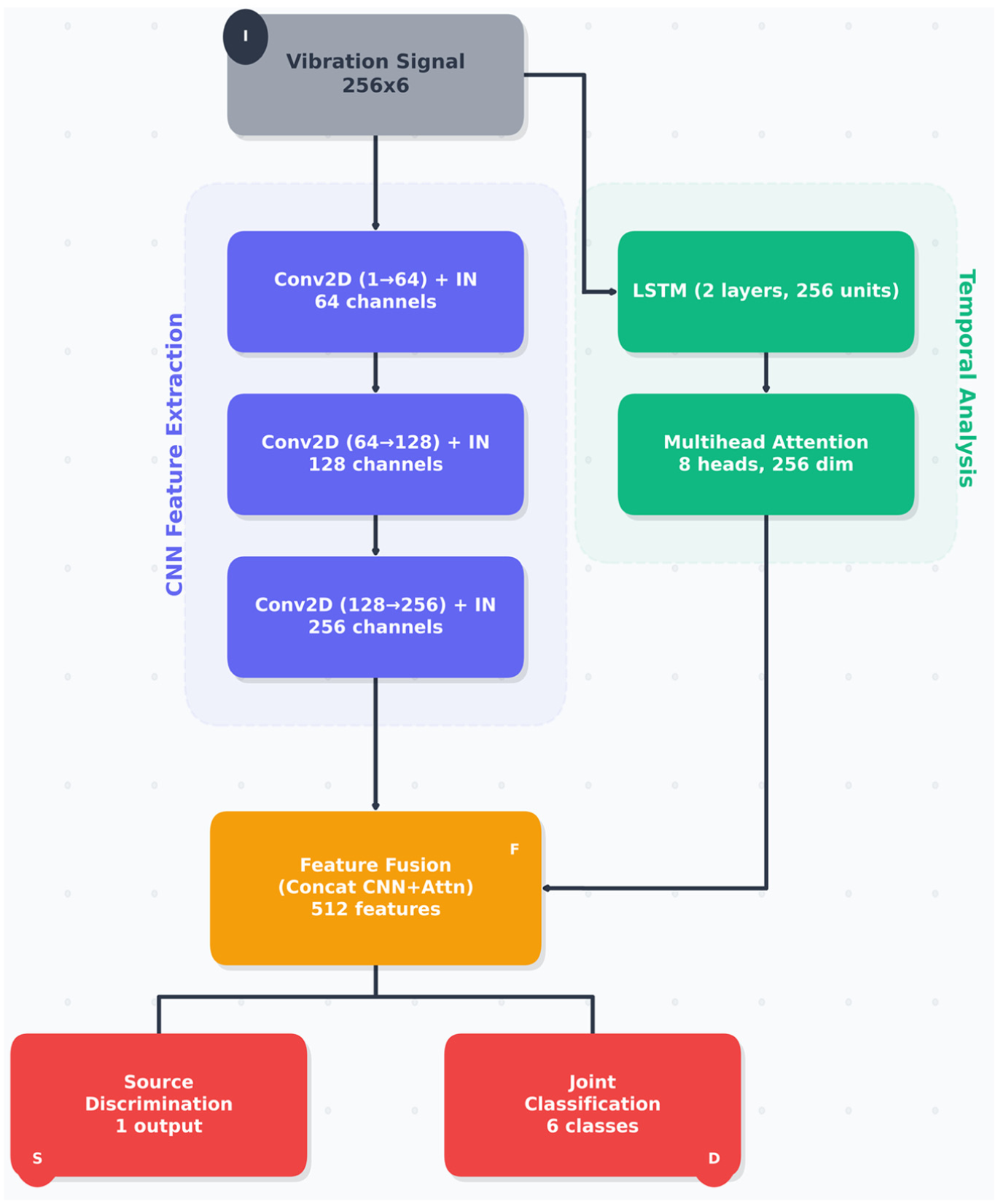
Discriminator architecture with dual output heads.
Beyond discrimination, the architecture supports a domain translation capability that enables transformation of vibration signals between different joint and structural state configurations within the same structure, as well as across structures of different material types. During intra-structure translation, the model learns to generate synthetic responses corresponding to alternative joint and structural state combinations belonging to the same physical structure. Given an input signal x
source
with conditions

where
The framework also supports cross-structure translation for adaptation between structures with different material properties or geometries. Structural domain indicators are included, and the generator learns to retain essential response characteristics while adapting to domain-specific attributes such as stiffness, damping, and modal behavior. For source and target domains m source and m target , the translation is defined as

and a reconstruction path is established through

These transformations provide the flexibility needed to generalize across different structural systems and extend the model’s applicability beyond a single test article.
These transformations allow the model to handle different structural systems and operate beyond a single test setup. The domain-translation step increases the available data by generating synthetic vibration responses for any combination of joint location, structural state, and domain. Instead of relying only on the limited set of tested configurations, the model can fill in a denser structural-response space, which supports data-driven SHM tasks. During training, each real sample x
real
is paired with randomly selected target conditions

which is evaluated for both realism and conditional correctness. The discriminator processes both real and generated signals together with their associated conditions, producing:


Here, p
real
and p
fake
denote the real/fake probabilities, while the conditional outputs p
joint
and
Training objective
The training objective guides the AT-StarGAN-GP model toward generating synthetic vibration responses that retain the structural and modal characteristics of the accelerometer measurements. The objective combines several complementary loss terms, each focusing on a different physical or statistical aspect of the vibration signals, including adversarial realism, conditional correctness, cycle consistency, signal preservation, modal structure, frequency-domain behavior, and discriminator stability.
Traditional error metrics such as mean squared error (MSE) or peak signal-to-noise ratio (PSNR) are not well suited for GAN-based SHM modeling, because exact pointwise matching is less relevant than preserving vibration characteristics such as resonant frequencies, damping behavior, and mode-shape patterns. For this reason, the training objective prioritizes frequency-domain and structural consistency, aligning the generator with the physical behavior of the system rather than amplitude-level similarity.
To achieve this, the model jointly optimizes the following loss functions
1. Adversarial loss: This loss encourages the generator to match the real data distribution while the discriminator learns to separate real and synthetic samples. The generator’s adversarial loss is
○ For the generator:

where x is the input data, c is the condition (damage scenario), and
○ For the discriminator:
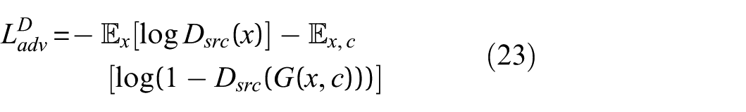
here x, is the real data,
The generator attempts to minimize the adversarial loss, while the discriminator maximizes it, leading to a more robust model.
2. Classification loss: This loss enforces that generated samples match the target class and that the discriminator correctly identifies the class of each input. It is defined as:

where
3. Cycle consistency loss: This loss enforces that a sample transformed to a target class and then mapped back to its source class remains consistent with the original input. It is defined as:

where x is the input data, c
s
is the source class, and c
t
is the target class.
4. Reconstruction loss: This loss requires the generator to reproduce the input signal when conditioned on its own class label. It is defined as:

where x is the input signal and c
s
is its source class.
This loss evaluates the generator’s ability to preserve the signal within its original class, ensuring that no unnecessary changes are introduced during reconstruction. It differs from identity loss by directly assessing reconstruction accuracy rather than only discouraging unwanted modifications during class transformations.
5. SVD loss: This loss encourages the generator to preserve modal characteristics during cycle reconstruction. It is defined as:
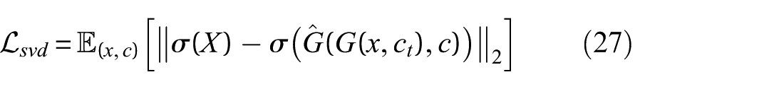
where
6. Frequency loss: This loss aligns the spectral content of generated signals with that of real signals by comparing their power spectral densities (PSDs). It is defined as:
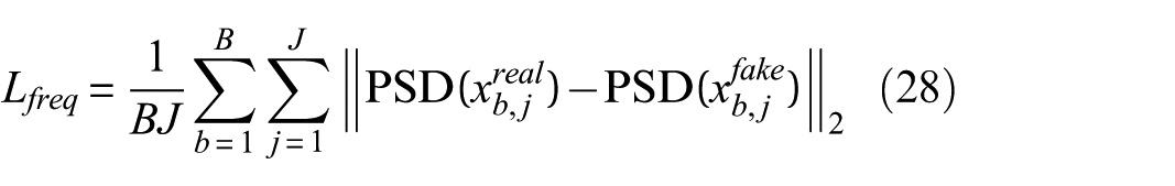
where B is the batch size and J is the number of accelerometers channels. Here
7. GP loss: This regularization term ensures that the discriminator satisfies the Lipschitz condition, which is necessary for stable training. The GP loss is given by:

where
This term helps maintain the stability of the training process by penalizing the discriminator for violating the Lipschitz constraint.
The total loss function for the generator and discriminator combines these individual losses, weighted by hyperparameters that control their relative importance. The overall loss for the generator and discriminator is expressed as:
• For the generator:
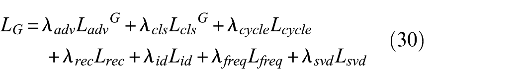
where
• For the discriminator:

where λ gp is the weight for the GP loss term.
Figure 4, illustrates the discriminator’s dual-headed architecture. Structural vibration signals are processed through two parallel paths. The CNN path extracts spatial features using three convolutional layers with increasing channel sizes (64, 128, 256) and sample normalization. The temporal path uses LSTM layers and an eight-head self-attention module to capture time-dependent patterns. The outputs from both paths are combined into a 512-dimensional feature vector, which is passed to two output heads: one for real/fake discrimination and one for damage-class prediction. This structure allows the discriminator to assess both signal authenticity and class consistency during training.
The architecture incorporates mechanisms to match frequency-domain characteristics, including PSD and singular-value patterns obtained from singular value decomposition (SVD). These constraints help reduce discrepancies between real and generated signals in the spectral domain, an area where time-domain accuracy alone may be insufficient for SHM tasks. An adaptive weighting scheme adjusts the influence of different loss terms based on signal quality metrics. This allows the model to operate under varying sensor noise levels without requiring extensive manual tuning.
Experimental evaluations indicate that the architecture preserves key frequency components more consistently than standard GAN baselines. It also shows improved damage-class discrimination compared with transformer-only models, while maintaining lower inference time. The attention mechanisms help identify generalizable structural features, which may support deployment across different structures, though further testing is needed to assess transfer-learning performance.
Overall, the dual-path design provides a combined spatial and temporal feature representation and incorporates frequency-domain constraints that are useful for SHM applications.
Training objectives and stability strategy
The data-processing stage converts raw vibration measurements into windowed segments for use in the AT-StarGAN-GP framework. The procedure preserves temporal relationships within each signal and spatial relationships across accelerometer channels, allowing the model to learn both aspects. The full workflow and architecture are shown in Figure 5.
AT-StarGAN-GP model architecture. AT-StarGAN-GP: attention-enhanced star generative adversarial network with gradient penalty.
The training objective is to generate synthetic structural-state data that maintain the main characteristics of the accelerometer responses. Several loss terms contribute to this objective. The adversarial loss encourages the generator to follow the distribution of real vibration signals. The classification loss enforces correct joint and structural-state labels. Cycle-consistency and identity losses help the model preserve important features when translating between states or reconstructing a signal under its original label. The SVD loss aligns the singular-value spectra of real and reconstructed samples, and the frequency-domain loss compares the PSDs of real and generated signals. A gradient-penalty term enforces the Lipschitz condition for stable discriminator training. Together, these losses guide the model toward producing structurally consistent synthetic responses.
Standard metrics such as MSE or PSNR are not well suited for vibration-signal evaluation, since SHM focuses on dynamic characteristics rather than point-wise waveform similarity. Frequency-domain comparisons based on PSDs or Fourier transforms provide a more relevant basis for assessment.
The architecture includes an adaptive hyperparameter mechanism that adjusts the loss weights using signal-quality metrics computed at a 128 Hz sampling rate. This helps the model remain stable under varying noise levels and maintain performance when operating on 256-sample windows with 50% overlap. The model preserves characteristic frequencies more reliably than standard GAN baselines, distinguishes structural-state effects better than transformer-only models, and runs at inference speeds suitable for edge-device deployment.
A dual-attention mechanism supports generalization across structures by identifying features that are common across joint–state combinations while allowing adaptation to specific structural characteristics. This reduces the amount of structure-specific calibration required, as illustrated in Figure 6.
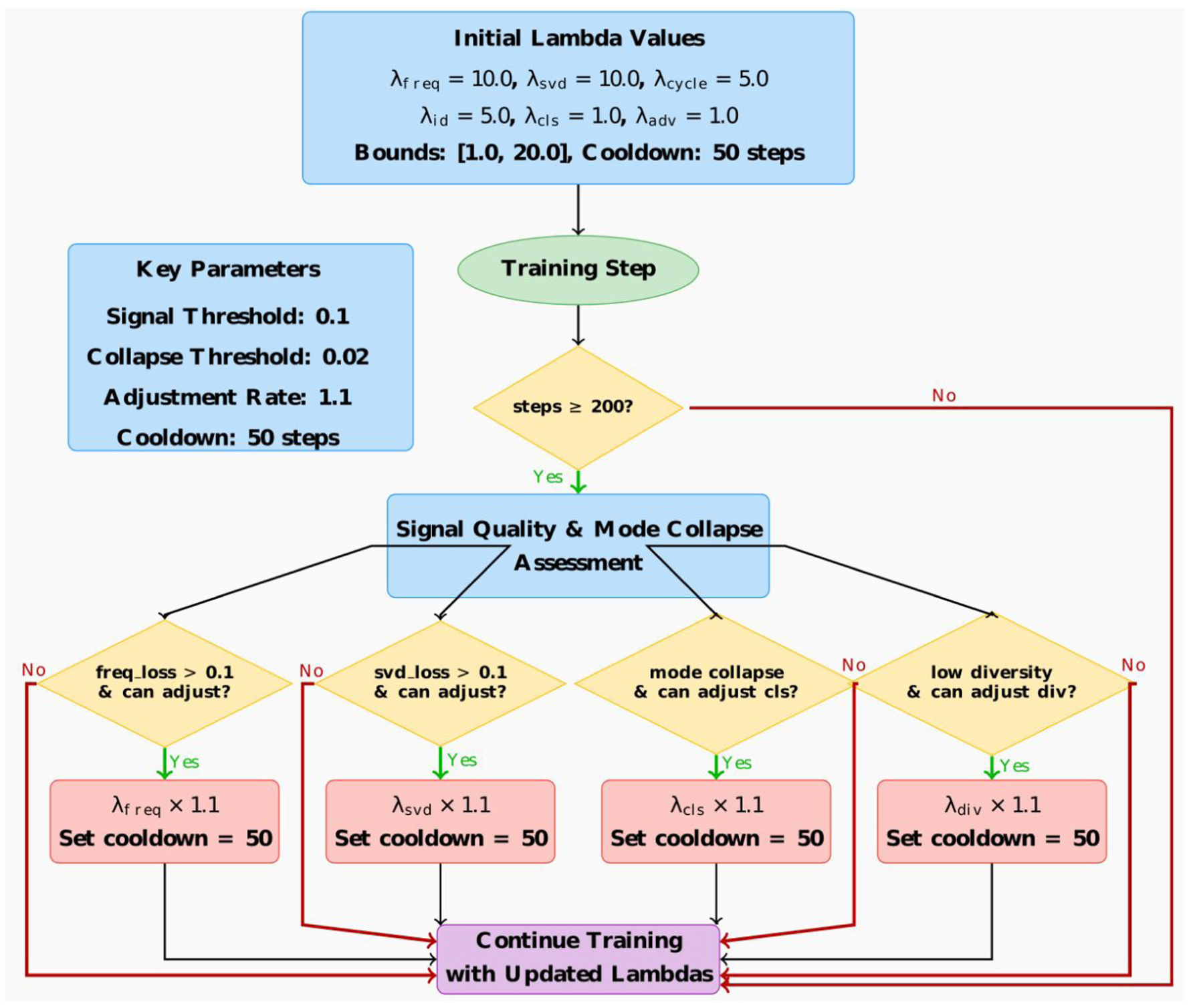
AT-StarGAN-GP: dynamic lambda adjustment strategy. AT-StarGAN-GP: attention-enhanced star generative adversarial network with gradient penalty.
To maintain stable training across translation tasks, AT-StarGAN-GP uses a dynamic optimization strategy that adjusts the lambda weights assigned to each loss component. Initial weights are set to 10.0 for the frequency and SVD losses, 5.0 for cycle-consistency and identity losses, and 1.0 for adversarial, classification, and diversity losses. After 200 training steps, the model begins monitoring SVD and frequency losses, with thresholds set at 0.1. When these thresholds are exceeded, the corresponding lambda values are increased by a factor of 1.1, subject to upper and lower limits of 20.0 and 1.0. A cooldown period of 50 steps prevents rapid changes. When signal-matching performance is low, the lambda values for adversarial, diversity, reconstruction, and classification losses are reduced so that the generator prioritizes structural and spectral consistency. Figure 6 illustrates the adjustment process.
Evaluation metrics
The evaluation of AT-StarGAN-GP focuses on metrics that capture dynamic and modal characteristics of structural vibration signals, rather than direct waveform matching. Since SHM emphasizes modal behavior, damping variations, and frequency shifts, the assessment uses representations that reflect these physical properties.
Generated signals are compared to real data using modal assurance criterion (MAC) and frequency response assurance criterion (FRAC) to evaluate mode shapes and frequency-response characteristics. PSD comparisons assess resonant frequencies and energy distribution, with Kolmogorov–Smirnov tests applied to quantify distributional similarity. Dynamic time warping (DTW) measures temporal alignment, while maximum mean discrepancy (MMD) compares signal distributions. Mode collapse is monitored throughout training using diversity metrics.
Model comparisons evaluate different conditioning strategies and assess component contributions through ablation studies. Convergence is tracked via Wasserstein distance and gradient norms, while computational efficiency is measured through training time, parameter count, and inference latency.
Generalization capability is tested across unseen-domain scenarios including unseen mass-position combinations, extrapolation beyond training ranges, cross-position transfer, and zero-shot translation. Noise robustness is assessed by adding progressive levels of Gaussian noise and measuring performance retention. Attention mechanisms are analyzed through localization accuracy, attention entropy, rollout visualizations, cross-domain KL divergence, and frequency band importance heatmaps.
Statistical validation employs cross-validation with Friedman and Nemenyi tests to confirm significance of performance differences. A composite score integrates seen domain, unseen domain, and noise-corrupted performance to balance accuracy, generalization, and robustness. Downstream utility is evaluated through damage classification tasks using different real-synthetic mixing ratios.
Overall, this evaluation framework characterizes the realism, structural validity, generalization capability, computational efficiency, and practical utility of generated vibration signals across multiple operational conditions and architectural configurations.
Results and discussion
In order to enable visual evaluation of AT-StarGAN-GP in capturing the structural dynamic behavior, Figure 7(a) to (j) present the first five mode shapes under all mass configurations, shown for the experimental reference data and the synthetically generated data. Each subfigure displays one mode shape. This qualitative comparison provides an initial check before quantitative evaluation of the modal parameters and helps confirm that the generated responses follow the main deformation patterns observed in the experiments.
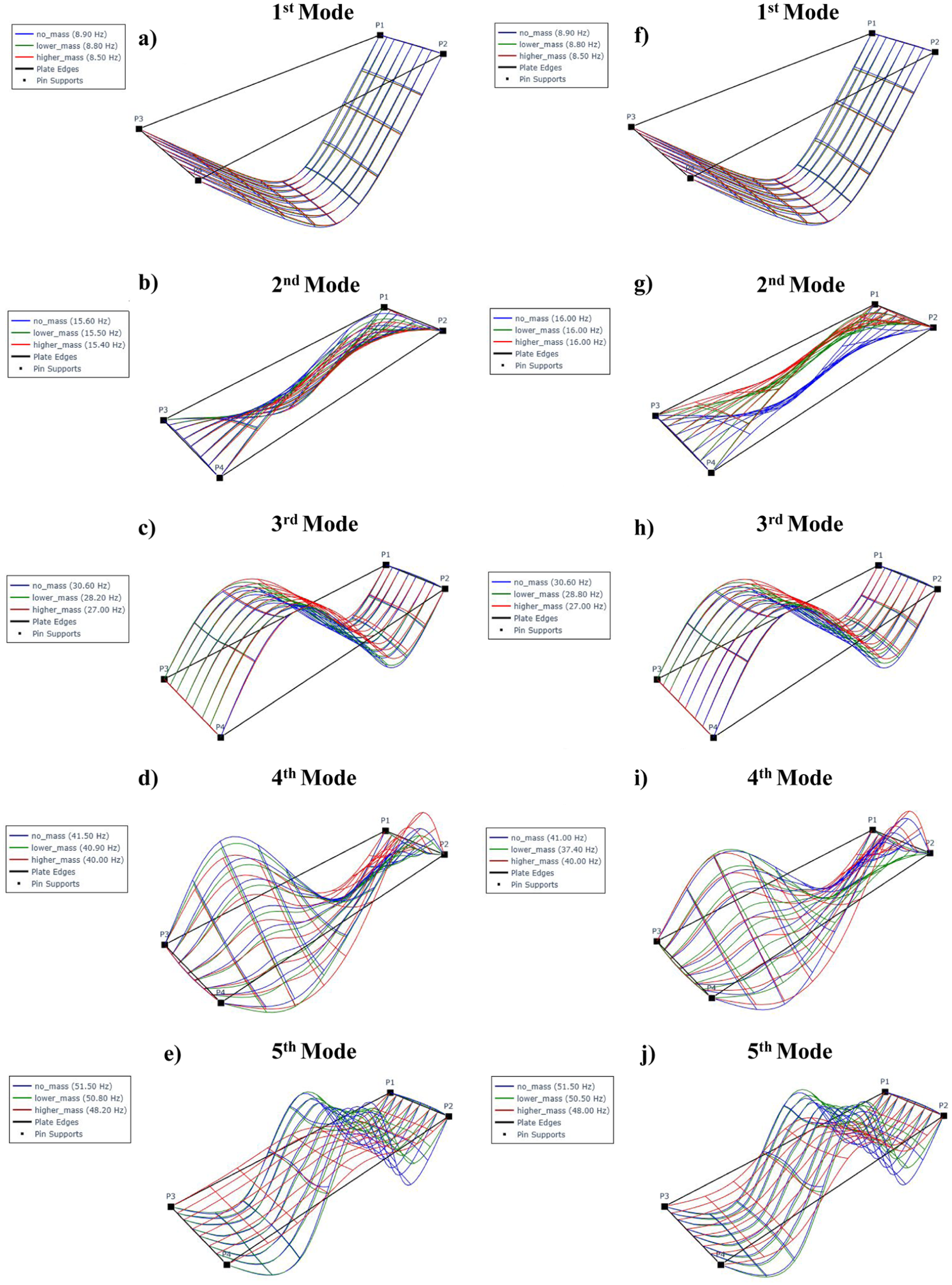
Comparative mode shapes for (a–e) experimental versus (f–j) AT-StarGAN-GP synthetic data across all mass configurations. AT-StarGAN-GP: attention-enhanced star generative adversarial network with gradient penalty.
In the generated second mode, the modal frequency remains constant at 16.00 Hz across all mass scenarios, regardless of the variation in mass. Although the corresponding mode shapes exhibit some similarity to the original (reference) mode shapes, there are noticeable discrepancies in their spatial characteristics which is associated with the torsional behavior. This suggests that the second mode is not significantly affected by the added masses.
The fourth mode exhibits a different trend. In this case, the configuration with lower mass yields a lower modal frequency compared to that with higher mass. Despite this variation in frequency, the fourth mode shapes remain quite similar to the actual mode shapes.
A common feature of both the second and fourth modes is their torsional nature. Since the additional masses were placed at the midpoints along the width of the structure, it is likely that these mass placements did not induce sufficient asymmetry or eccentricity to significantly influence the torsional modes. This could account for the limited sensitivity of the second mode frequency to mass variation and the relatively small changes in the fourth mode shape and frequency.
The comparison between experimentally identified and synthetically generated modal parameters for the no-mass configuration, shown in Figure 8 and detailed in Table 1, indicates that the model preserves the main dynamic characteristics of the structure. The natural frequencies in Table 1, show small differences between the synthetic and experimental results, staying within 2.6% for all identified modes. Modes 1, 3, and 5 show no difference, while modes 2 and 4 differ by 2.6 and 1.2%. The SVD comparison in Figure 8, is consistent with these observations, showing similar patterns between original and synthetic data.
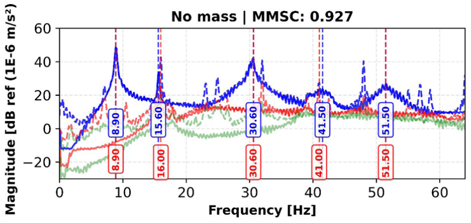
SVD comparison between original and synthetic data for no mass scenario, with identified natural frequencies. SVD: singular value decomposition.
Natural frequencies and damping ratios for no mass scenario: comparison between original and synthetic data, including the percentage differences in natural frequencies and damping ratios.
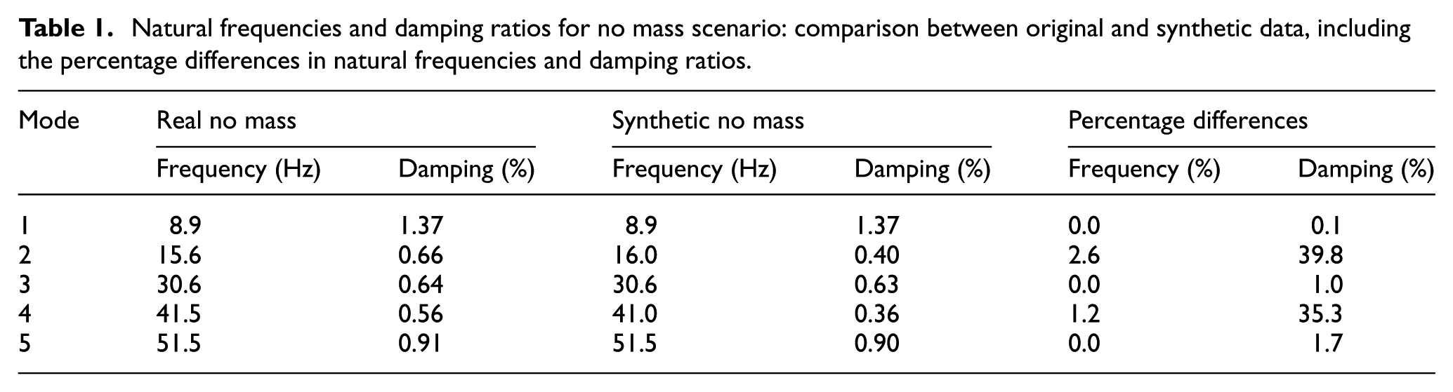
The damping ratio comparison in Table 1 shows more variation. Modes 1, 3, and 5 have small differences that range from 0.1 to 1.7%, while modes 2 and 4 show larger discrepancies of about 35 to 40%. This outcome is consistent with previous observations, where damping-related quantities were found to be more sensitive and more difficult to reproduce accurately than natural frequencies. 43
Despite the observed differences, the overall mean magnitude squared coherence (MMSC) value of 0.927 indicates a good level of agreement between the synthetic and experimental modal data. Since this value is above the commonly used validation threshold of 0.8, it meets typical criteria for modal comparison. The close match in natural frequencies, together with reasonably consistent damping estimates, suggests that the generated signals can be used to support experimental datasets, particularly in situations where measurements are limited.
The comparative analysis of modal parameters for the lower_mass_pos1 configuration, shown in Figure 9 and summarized in Table 2, indicates that the AT-StarGAN-GP model reproduces the main dynamic features of the modified structural condition. The SVD results in Figure 9 show that the synthetic data reflect the natural frequency distribution observed in the experimental measurements. As reported in Table 2, four of the five identified modes (modes 1, 3, 4, and 5) show no frequency difference (0.0%), while mode 2 differs by 3.2%. These values indicate that the model captures the frequency shifts associated with the added mass.
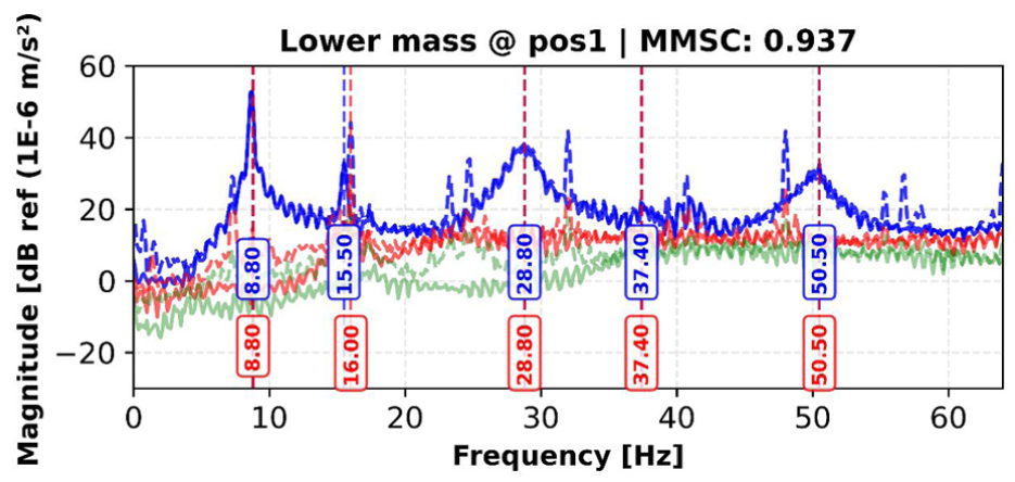
SVD comparison between original and synthetic data for lower mass at position 1 scenario, with identified natural frequencies. SVD: singular value decomposition.
Natural frequencies and damping ratios of lower mass scenario, synthetic lower mass at position 1 scenario, and percentage differences of natural frequencies and damping ratios between original and synthetic scenario.
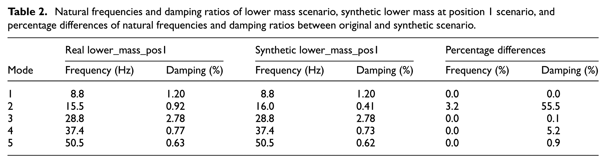
The damping ratio comparison in Table 2 shows a wider range of differences. Modes 1 and 3 exhibit small damping differences of 0.0 and 0.1%, while modes 4 and 5 differ by 5.2 and 0.9%, respectively. Mode 2 shows a larger discrepancy of 55.5%, suggesting reduced consistency for that mode. The overall MMSC value of 0.937 indicates good agreement between the synthetic and experimental modal properties and is slightly higher than the value obtained for the no-mass case. Since this value is above the commonly used 0.8 validation threshold, it meets standard criteria for modal comparison.
The close match in natural frequencies and generally acceptable damping estimates show that the model can represent the influence of added mass on the structural response. For completeness, the results for the lower_mass_pos2 and lower_mass_pos3 configurations, which follow trends similar to those of lower_mass_pos1, are provided in Appendix A. These findings indicate that the generative approach can be used to supplement experimental data in cases where multiple mass configurations cannot be tested extensively.
The modal validation results in Table 3 show the comparison between experimental and synthetic acceleration data for the higher_mass_Pos1 configuration. Modes 1, 3, and 4 exhibit no frequency difference (0.0%) at 8.5, 27.0, and 40.0 Hz, respectively. Mode 5 differs by 0.4% (48.2 vs 48.0 Hz), and mode 2 differs by 3.9% (15.4 vs 16.0 Hz). These values indicate that the synthetic data follow the frequency shifts associated with the added mass.
Natural frequencies and damping ratios of higher mass scenario, synthetic higher mass at position 1 scenario, and percentage differences of natural frequencies and damping ratios between original and synthetic scenario.
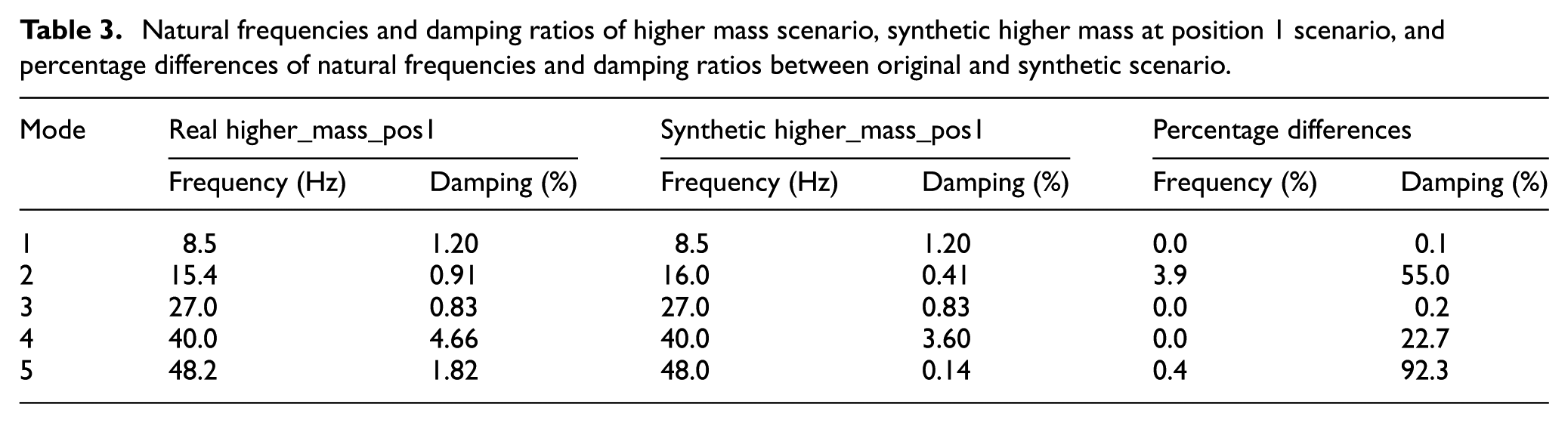
Damping ratios show greater variation across modes. Modes 1 and 3 have small differences of 0.1 and 0.2%, while mode 4 differs by 22.7%. Modes 2 and 5 show larger discrepancies of 55.0 and 92.3%. The overall MMSC value is 0.964 (Figure 10), indicating a high level of agreement in mode shapes between the experimental and synthetic data.
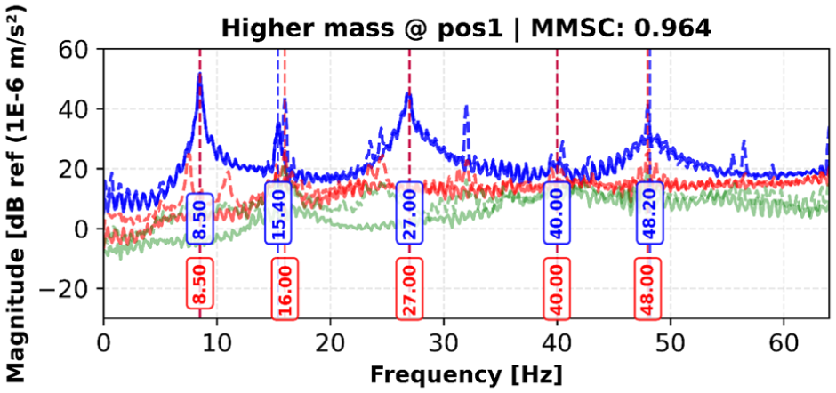
SVD comparison between original and synthetic data for higher mass at position 1 scenario, with identified natural frequencies. SVD: singular value decomposition.
Results for the higher_mass_pos2 and higher_mass_pos3 configurations, which show trends similar to higher_mass_pos1, are provided in Appendix A. The comparisons indicate how frequency values, damping ratios, and mode shapes vary across experimental and synthetic datasets under increased mass conditions.
The validation results across the different mass configurations show that the network produces synthetic acceleration data that generally preserves the main structural dynamic features. Natural frequencies are reproduced with small deviations, mostly remaining below 3.9%, and the MMSC values fall between 0.894 and 0.980, indicating close agreement in mode shapes. Damping ratio estimates vary more noticeably, particularly for intermediate modes under higher mass conditions. Overall, the frequency accuracy and mode shape coherence are consistent across the tested scenarios, while damping shows greater sensitivity to mass changes. The results indicate that the generated data reflects the expected effects of altered stiffness and mass distribution and maintains the primary characteristics relevant for structural state assessment and system identification.
Label conditioning mechanisms and component ablation study
Two analyses were carried out to examine how conditioning strategies and specific generator components affect the behavior of the AT-StarGAN-GP framework: (i) an evaluation of different label-conditioning mechanisms and (ii) an ablation study examining the roles of the attention module and the GP.
Label conditioning strategy evaluation
Four conditioning approaches were examined under the same architecture and training setup: Concat, FiLM, AdaIN, and CIN. Joint-state embeddings were used as conditioning inputs. Performance was evaluated using modal, temporal, distributional, and spectral measures relevant to vibration-based SHM, with results for the steel dataset presented in Table 4.
Comparison of conditioning methods via performance metrics.
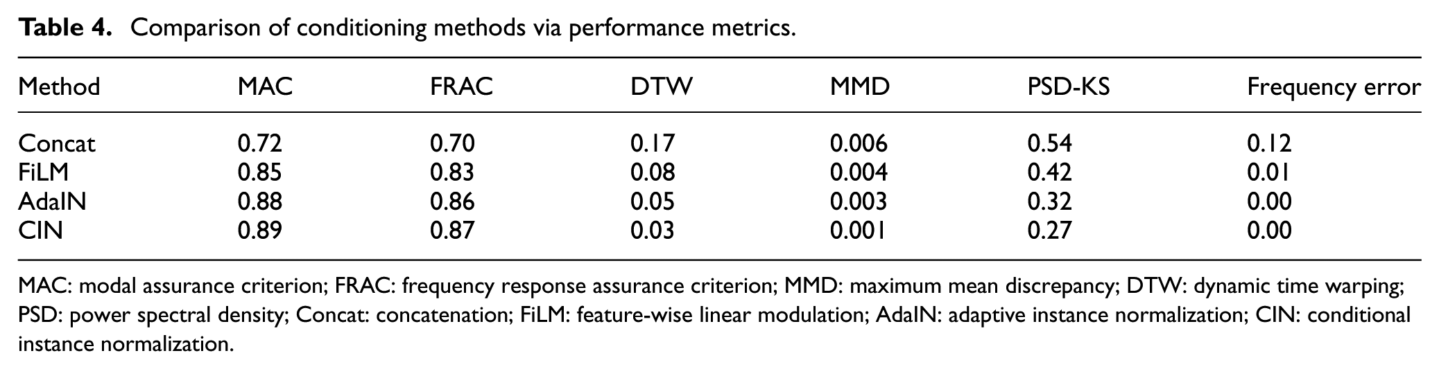
MAC: modal assurance criterion; FRAC: frequency response assurance criterion; MMD: maximum mean discrepancy; DTW: dynamic time warping; PSD: power spectral density; Concat: concatenation; FiLM: feature-wise linear modulation; AdaIN: adaptive instance normalization; CIN: conditional instance normalization.
CIN yields the highest MAC (∼0.89) and FRAC (∼0.87) values among the tested approaches. It also shows the lowest DTW distance (0.03) and lower distributional and spectral discrepancies (MMD 0.001, PSD-KS 0.27, frequency error 0.00). AdaIN follows with MAC 0.88, FRAC 0.86, and DTW 0.05. FiLM and Concat produce comparatively higher errors across the evaluated metrics.
Component contribution ablation study
Following the conditioning strategy evaluation, the contribution of individual architectural components was examined. The radar chart in Figure 11 summarizes the ablation results for the AT-StarGAN-GP generator across all mass conditions. The full model reports the highest MAC value (about 0.89) and a mode-collapse rate of around 2.6%, with relatively consistent performance across modal, temporal, and distributional metrics. Removing the attention mechanism lowers MAC by approximately 6.1% and increases mode collapse to 4.8%. Excluding the GP reduces MAC by about 4.8% and raises mode collapse to 12.4%. When both components are removed, the reductions are largest, with a MAC decrease of roughly 9.6% and a mode-collapse rate of 15.2%. A Friedman test indicates that these differences are statistically significant (p = 0.0018).
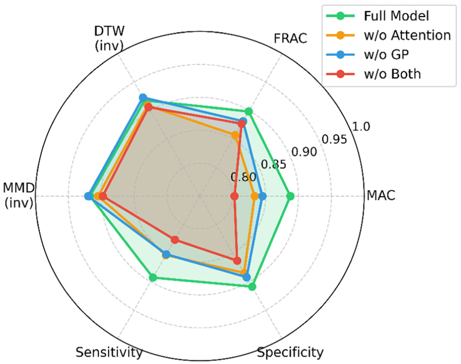
Ablation of attention and GP in AT-StarGAN-GP. GP: gradient penalty; AT-StarGAN-GP: attention-enhanced star generative adversarial network with gradient penalty.
Mass-specific effects of component removal are shown in Figure 12. The results show the component-wise ablation outcomes for higher mass and lower mass conditions. For the higher mass cases, removing the attention mechanism reduces MAC by approximately 5.9%, and removing the GP reduces MAC by about 4.1%. When both components are removed, the MAC decrease is around 8.3%. Mode collapse is low for the full model (2.2%).
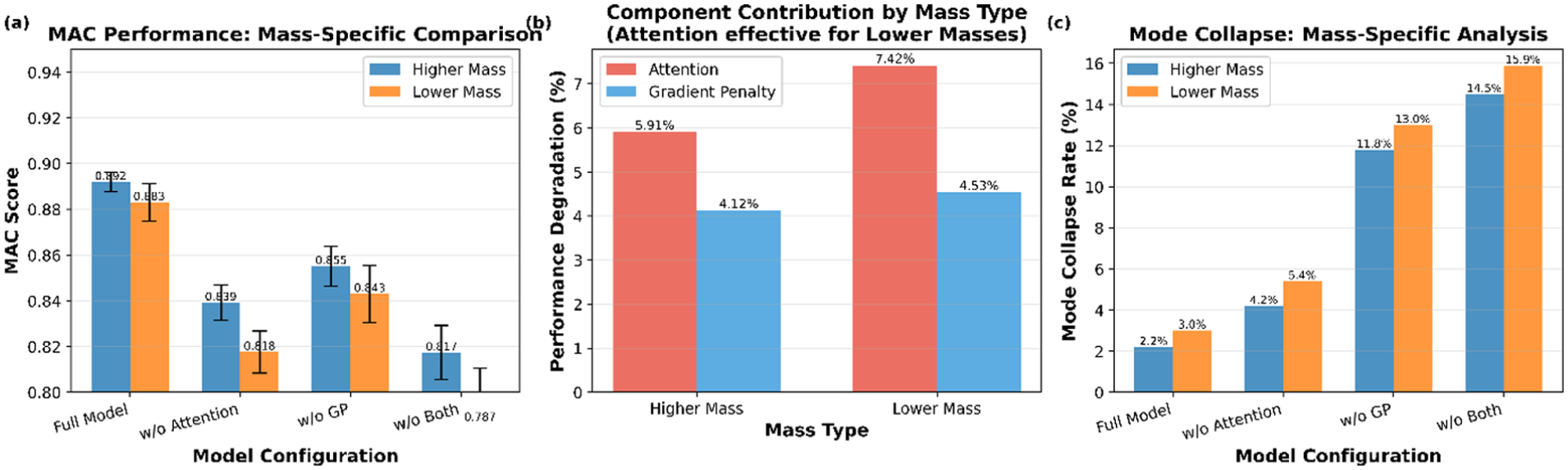
Mass-specific impact of attention and GP in AT-StarGAN-GP, showing: (a) MAC performance: mass-specific comparison, (b) component contribution by mass type, and (c) mode collapse: mass-specific analysis.
For the lower mass cases, attention removal leads to a MAC reduction of roughly 7.4%, while GP removal results in a reduction of about 4.5%. The combined removal produces a decrease of approximately 10.9%, with mode collapse reaching up to 15.9% in the w/o both configuration.
Convergence characteristics of multi-domain GAN architectures
Following the component ablation analysis, the convergence behavior and computational requirements of different multi-domain architectures were compared. Figure 13 summarizes the convergence and scalability characteristics of the evaluated models. Figure 13(a) shows the convergence trajectories over 50,000 training iterations. AT-StarGAN-GP reaches stable behavior at around 18,000 iterations with a final Wasserstein distance of 0.032. WGAN-GP converges near 32,000 iterations with a distance of 0.048, while CycleGAN converges around 42,000 iterations with a distance of 0.063. The corresponding gradient norms in Figure 13(a) indicate that AT-StarGAN-GP maintains relatively consistent gradients compared to the higher-variance patterns seen in the other methods. Figure 13(b) reports the associated computational costs. The unified architecture of AT-StarGAN-GP requires training a single generator–discriminator pair, whereas pairwise methods require 210 separate models for the 15-domain setting. This leads to a total training time of 13.8 h for AT-StarGAN-GP compared with 13,524 h for CycleGAN. Model complexity results in Figure 13(c) show the differences in architectural scale between unified and pairwise approaches. The single-model design of AT-StarGAN-GP reduces overall parameter count and avoids the replication required by CycleGAN-style frameworks. Lastly, Figure 13(d) presents inference latency. AT-StarGAN-GP processes samples at 3.2 ms per instance, while CycleGAN reaches 8.0 ms. The multi-attribute classification trajectories in Figure 13(a) indicate that AT-StarGAN-GP reaches a final score of 0.91, compared to 0.88 for WGAN-GP.
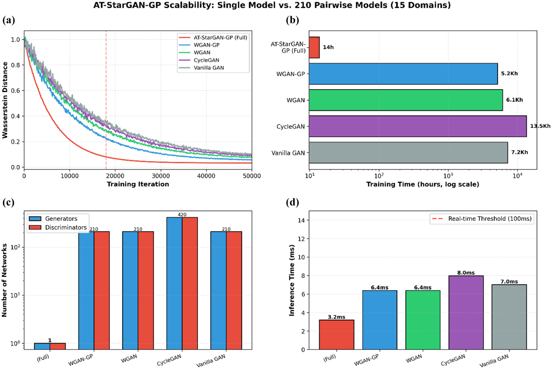
AT-StarGAN-GP convergence and scalability analysis: (a) convergence speed, (b) computational cost, (c) model complexity and (d) real-time performance. AT-StarGAN-GP: attention-enhanced star generative adversarial network with gradient penalty.
Spectral fidelity and training dynamics
The preceding convergence analysis focused on training efficiency metrics. This section examines the quality of generated signals through their spectral characteristics and associated training stability. Figure 14 presents PSD overlays of real and generated responses for each conditioning method. CIN maintains the dominant modal peaks and damping patterns with close alignment to the experimental spectra. AdaIN preserves peak locations but shows slightly broader spectral distributions. FiLM introduces small frequency shifts in higher modes, and Concat produces broader peaks with occasional high-frequency components.
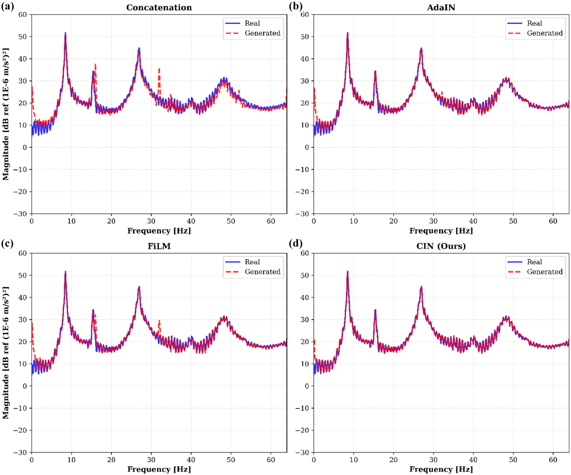
PSD comparison across conditioning methods: (a) Concat, (b) AdaIN, (c) FiLM and (d) CIN. Conact: concatenation; PSD: power spectral density; AdaIN: adaptive instance normalization; CIN: conditional instance normalization; FiLM: feature-wise linear modulation.
The relationship between spectral quality and training dynamics was further examined through variance and gradient-penalty metrics. Training stability, evaluated through feature variance and minibatch standard deviation (Figure 15(a) and (b)), reveals that Conact suffers rapid variance collapse, FiLM exhibits intermittent dips, AdaIN maintains moderate stability, and CIN consistently preserves high feature variance. Gradient-penalty behavior (Figure 16) confirms that CIN achieves rapid convergence with minimal critic gradient oscillation, while AdaIN stabilizes training slightly slower, and Conact and FiLM show persistent instabilities.
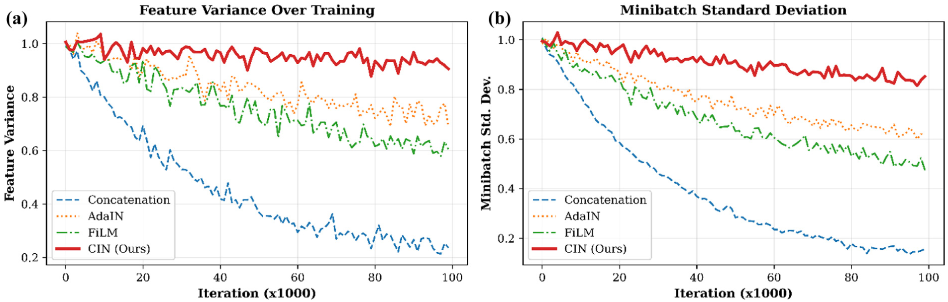
Mode collapse diagnostic analysis, showing: (a) feature variance over training and (b) minibatch standard deviation
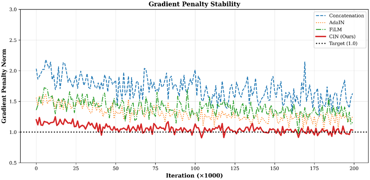
GP stability and convergence analysis. GP: gradient penalty.
Statistical distribution preservation
Beyond spectral alignment, statistical distribution preservation was assessed through Kolmogorov–Smirnov tests. The Kolmogorov–Smirnov analysis in Figure 17 assesses how well each conditioning method preserves the statistical structure of SVD-based PSD envelopes across seven damage classes. In Figure 17(a), Conact and FiLM consistently show large KS (Kolmogorov-Smirnov) divergences, typically above 0.45. For example, in the higher_mass_pos3 class, Conact reaches 0.582. CIN shows the lowest KS values overall: six of the seven classes remain below the threshold of 0.30, with only the No_mass class slightly above at 0.310. AdaIN exhibits a mixed outcome, with five classes failing and two classes passing the threshold.
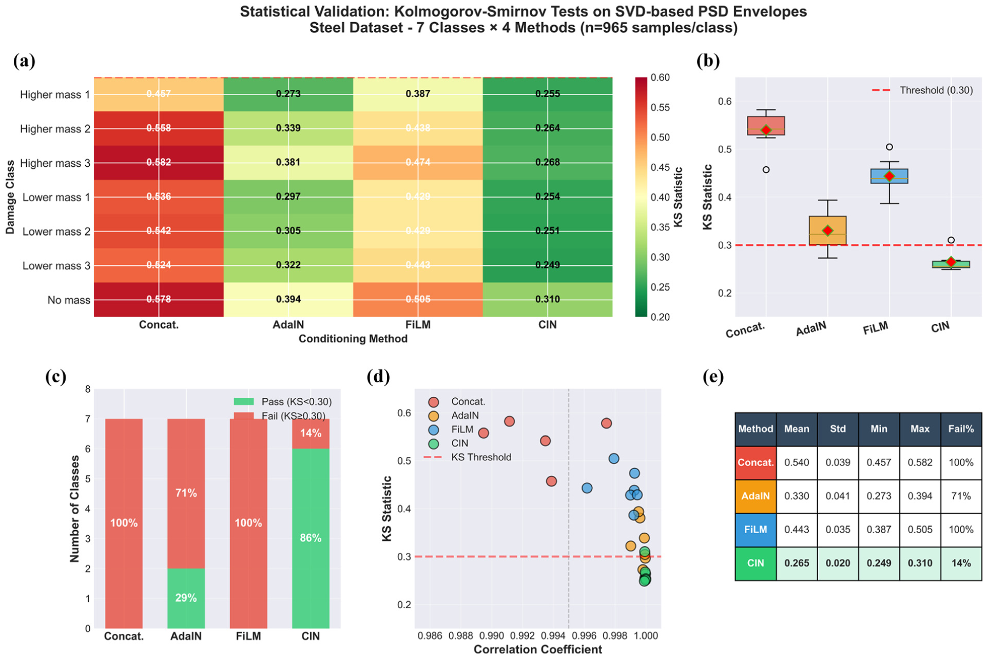
Statistical validation of vibration responses using Kolmogorov-Smirnov tests on SVD-based PSD envelopes, showing: (a) KS statistics heatmap, (b) KS distribution by method, (c) pass/fail rate, (d) correlation vs KS divergence, and (e) summary statistics table via Kolmogorov–Smirnov tests.
The results in Figure 17(b) clear differences in the KS distributions across methods. CIN has the lowest mean KS value (0.265) and the smallest spread (standard deviation 0.020). In contrast, Conact and FiLM produce wide distributions with all values above the 0.30 threshold. AdaIN lies between these patterns, with a mean KS of 0.330 and a noticeably larger variance across the classes. For CIN, the entire boxplot stays below the threshold except for a single borderline case. A similar trend appears when looking at the pass and fail counts in Figure 17(c). CIN is the only method that passes most tests (86%), whereas AdaIN passes two of the seven classes (29%). FiLM and Conact do not meet the threshold for any class. This indicates that, aside from CIN, none of the evaluated methods reliably reproduce the envelope distributions for the tested damage scenarios. Figure 17(d) compares KS divergence with correlation. All methods achieve very high correlation values (above 0.987), yet their KS statistics vary substantially, spanning a range of 0.275. For example, Conact reaches a mean correlation of 0.988 but has the highest KS divergence (0.540). CIN shows both near-unity correlation (0.99995) and the lowest KS values. In the scatter distribution, CIN occupies the region associated with both high correlation and low KS, while Conact and FiLM are concentrated in areas that reflect greater distributional mismatch. Figure 17(e) aggregates these observations: CIN has the lowest mean KS (0.265), the lowest standard deviation (0.020), the lowest maximum KS (0.310), and the lowest failure rate (14%). The other methods exhibit higher means, broader spreads, and substantially larger failure rates, with Conact and FiLM failing all tests. Taken together, the results show that even when correlation is consistently high, it does not reflect differences in distributional structure, whereas the KS statistic provides a clearer indication of how well each method preserves the underlying statistical patterns.
Attention mechanism impact on localization
Having examined conditioning strategies and overall performance metrics, the specific contribution of the attention mechanism to damage localization was analyzed. Figure 18(a) reports localization accuracy for the model with and without the attention module. Scores increase from 0.4538 ± 0.1162 to 0.6097 ± 0.1096, a 34.35% difference. Class-wise changes span 22.52–97.85% (mean 39.10 ± 24.77%). A positional pattern is evident: for both mass levels, Pos1 yields the highest accuracy, while Pos2 and Pos3 form a closely grouped pair at lower values. In the higher-mass case, scores reach 0.6675 at Pos1 (41.85% increase) and about 0.525 at Pos2 and Pos3 (around 27.6%). The lower mass case shows a similar trend, with 0.7847 at Pos1 (33.40%) and approximately 0.650 at Pos2 and Pos3 (around 22.7%). The no-mass class shows the largest relative change, rising from 0.2353 to 0.4655 (97.85%).
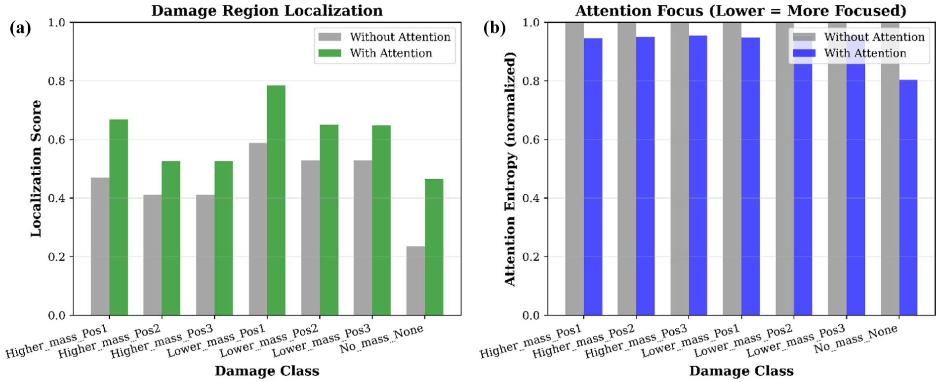
With versus without attention: (a) localization and (b) focus comparison.
Figure 18(b) provides the corresponding attention-entropy results. Without attention, all classes have an entropy of 1.0000. With attention, entropy decreases to 0.9302 ± 0.0559 on average, a 6.98% reduction. Most classes fall between 4.50 and 5.36% reduction, while the no-mass class shows a larger 19.63% decrease. A consistent positional ordering appears across both mass groups: Pos1 exhibits the lowest entropy values (0.946–0.948), followed by Pos2 (0.950–0.952) and Pos3 (0.954–0.955). These results indicate how the attention module changes the distribution of weights across the temporal sequence.
Multi-type attention rollout analysis
To understand how different attention mechanisms process structural response data, a detailed rollout analysis was conducted for a representative damage case. The spectrotemporal behavior of the Higher_mass_Pos1 case is shown in Figure 19(a), where the original spectrogram spans 0–64 Hz over a 0–0.25 s duration with a resolution of 17 frequency bins and three time steps. Energy levels range from −45.36 to −13.32 dB (mean −26.39 dB, SD (Standard Deviation) 7.74 dB), with most activity concentrated in the lower and mid-frequency bands, which aligns with the expected modal pattern under added mass.
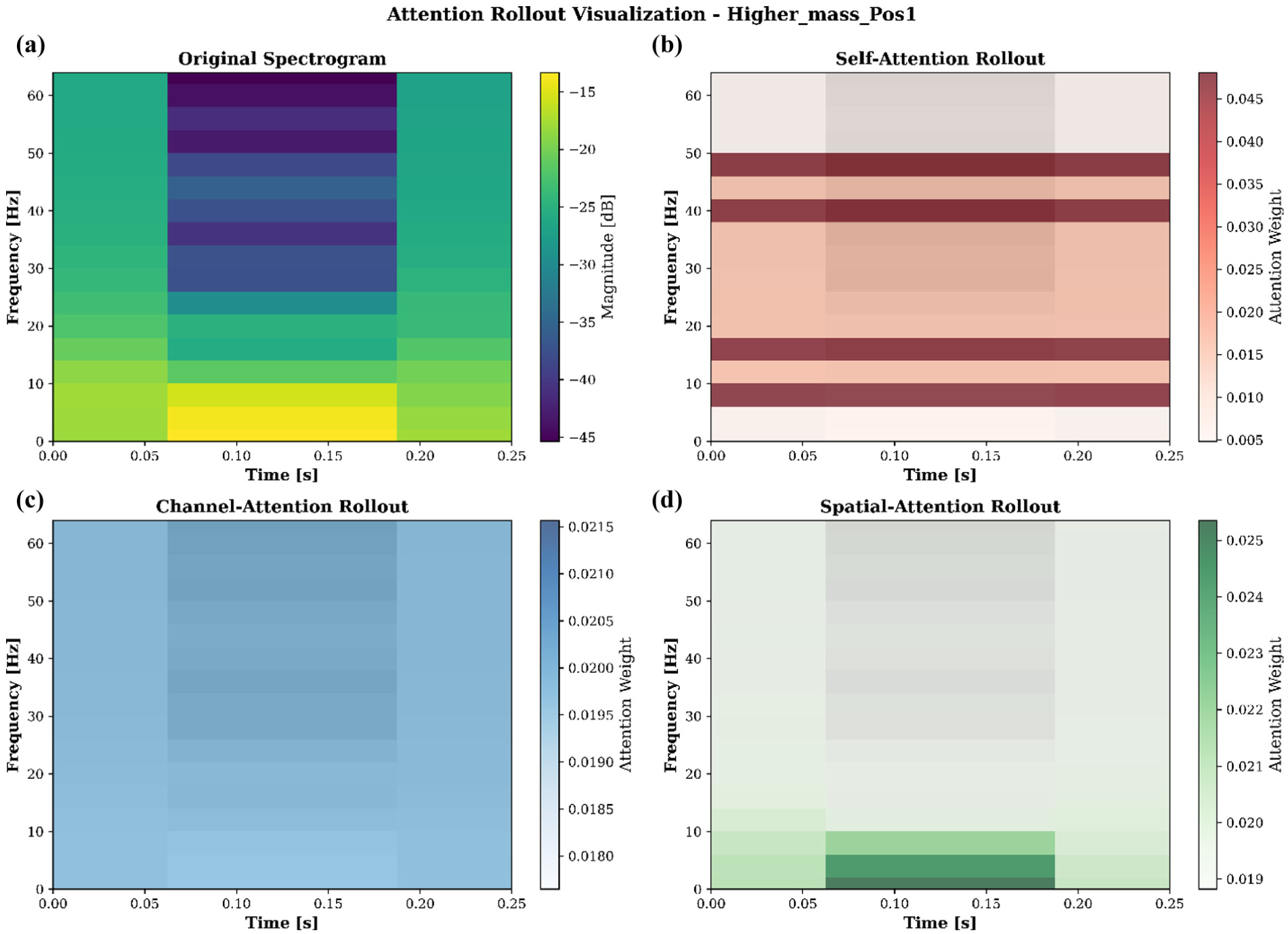
Attention rollout visualization, showing: (a) original spectrogram, (b) self-attention rollout, (c) channel-attention rollout, and (d) spati al-attention rollout
The self-attention rollout in Figure 19(b) indicates how frequency content is weighted. Values range from 0.0048 to 0.0481 (mean 0.0196), with the highest emphasis around 8 Hz at 0.125 s. The distribution shows a clear weighting toward the 8–16 Hz band (0.0371 on average), followed by reduced levels in the 16–32 Hz (0.0223) and 32–64 Hz (0.0180) ranges, reflecting how the model allocates attention to frequency regions where mass-related changes typically appear. Channel-attention results in Figure 19(c) are uniform for this example, with weights fixed at 0.0196 (SD 0.0000). This indicates that all sensor channels contribute equally in this configuration, with no measurable channel-selective behavior. The spatial-attention rollout in Figure 19(d) distributes weights across time and frequency within a narrow interval (0.0188–0.0254; SD 0.0013). Small variations highlight consistent but modest emphasis on localized time-frequency regions. The very low temporal and frequency variances (0.0 and 0.000001) suggest a controlled and coherent weighting pattern instead of isolated peaks.
Overall, the three attention components address different aspects of the input: self-attention highlights frequency bands affected by the added mass, spatial attention refines weighting across the time-frequency plane, and channel attention keeps the sensor contributions balanced.
Cross-domain alignment via attention
Following the rollout analysis, the effectiveness of attention mechanisms in reducing distributional shift between structural states was quantified. The effect of the three attention mechanisms on cross-domain feature alignment is evaluated using KL divergence as a measure of distributional shift. Absolute KL values for three domain pairs (Higher_mass → Lower_mass at Pos1 and Pos2, and No_mass → Higher_mass at Pos1) are presented in Figure 20(a), and the corresponding mitigation ratios relative to the no-attention baseline are summarized in Figure 20(b).
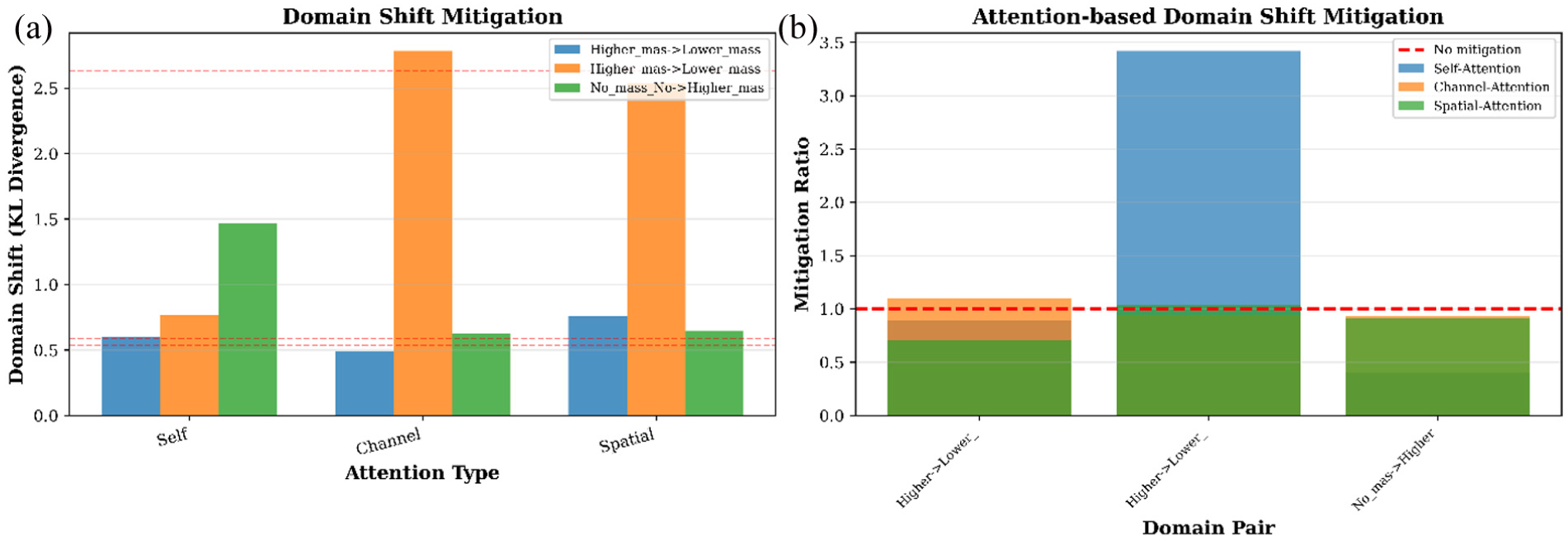
Attention-based domain shift mitigation: (a) domain shift (KL divergence) across attention types and (b) mitigation ratios compared to no-attention baseline
Across all domain pairs, the baseline KL divergence (no attention) averages 1.2515. Self-attention reduces this divergence to 0.9449 on average, representing a 24.5% decrease and a mean mitigation ratio of 1.57×. The largest reduction occurs in the Higher_ mass_Pos2 → Lower_mass_Pos2 transfer, where self-attention achieves a 3.42× decrease. Channel-attention remains near baseline, with a mean mitigation ratio of 0.99× and a slight increase in KL divergence to 1.2990, while spatial-attention shows a similar trend with a mean mitigation ratio of 0.88× and divergence of 1.3146.
Scenario-specific differences are observed. In the No_mass_None → Higher_mass_Pos1 transfer, self-attention increases the KL divergence (0.401×), whereas channel- and spatial-attention stay close to baseline levels (0.93–0.91×). These results reflect how each attention mechanism interacts with the spectral structure of the domain shift: self-attention tends to reduce shifts effectively when mass-related spectral changes dominate, but its impact varies when additional modal complexity is present in the target domain.
Frequency band attention patterns
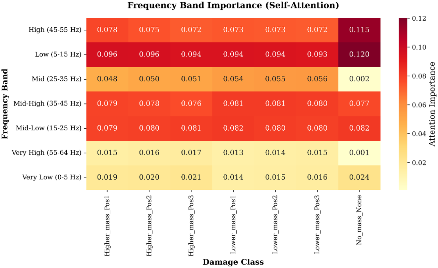
Complementing the cross-domain analysis, the attention distribution across frequency bands was examined to identify which spectral regions are prioritized across different structural states. The frequency band importance map (Figure 21) illustrates attention trends across all structural states. The Low (5–15 Hz) band consistently receives the highest attention in all mass-altered conditions, with values ranging from 0.0929 to 0.0962. This corresponds to the expected downward shift of modal energy when additional mass is introduced, showing that the spectral regions most affected by mass loading are prioritized. The undamaged state shows a similar concentration, though with higher variance and an elevated peak (0.1203), reflected in a more diffuse color distribution.
Damage-sensitive frequency band attention heatmap.
Mid-frequency bands display more nuanced, class-dependent variations. The Mid (25–35 Hz) band receives moderate but uneven attention, with elevated values for lower mass cases, such as 0.0558 for Lower_mass_Pos3, visible as localized warm regions. Mid-Low (15–25 Hz) and Mid-High (35–45 Hz) bands are nearly uniform across classes, with low variance (0.001–0.002), indicating they are generally informative but not discriminative for damage types. Very High (55–64 Hz) and Very Low (0–5 Hz) bands consistently show low attention (means of 0.0130 and 0.0186), reflecting limited relevance for distinguishing mass-induced changes. Minor localized increases, for example Higher_mass_Pos3 in the Very High band or No_mass in the Very Low band, correspond to small spectral irregularities in the signals.
The statistical summary supports the visual patterns. Damaged classes cluster around similar mean importance levels (∼0.059), whereas the undamaged state shows greater spread (standard deviation 0.0509), consistent with its uneven coloration. Across all classes, the Low band is the most prominent, while the Very High and Very Low bands are least emphasized. Overall, the attention allocation highlights frequency regions containing structurally relevant information while down-weighting those dominated by noise or non-informative content.
Comprehensive performance comparison
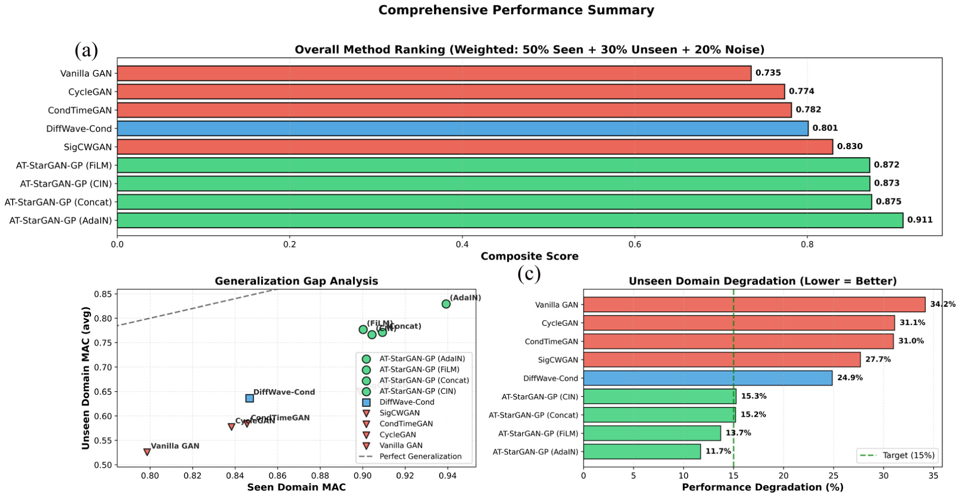
With detailed analyses of individual components and mechanisms complete, an overall comparison of all evaluated methods was conducted. Figure 22(a), the updated composite scores (50% seen, 30% unseen, 20% noise) place the AT-StarGAN-GP variants at the top. AdaIN reaches 0.9109, followed by Concat at 0.8746, CIN at 0.8725, and FiLM at 0.8723. The remaining baselines fall into a lower performance range: SigCWGAN at 0.8295, DiffWave-Cond at 0.8011, CondTimeGAN at 0.7816, CycleGAN at 0.7737, and Vanilla GAN at 0.7349.
Comprehensive performance summary: (a) overall method ranking, (b) generalization gap analysis, and (c) unseen domain degradation comparison.
Generalization patterns are shown in Figure 22(b) through the seen–unseen MAC scatter plot. The AT-StarGAN-GP variants cluster near the diagonal, indicating comparatively small differences between seen and unseen performance. AdaIN records 0.9392 (seen) and 0.8293 (unseen), with a gap of 0.1100. FiLM follows with 0.1234, and CIN and Concat fall between 0.1380 and 0.1382. The baselines display wider gaps: DiffWave-Cond at 0.2106, SigCWGAN at 0.2488, SigCWGAN at 0.2620, CycleGAN at 0.2609, and Vanilla GAN at 0.2729.
Degradation percentages for the unseen domain, provided in Figure 22(c) follow the same general ordering. The AT-StarGAN-GP variants show lower drops, ranging from 11.71% for AdaIN to 15.26% for CIN. The baselines experience larger reductions, with DiffWave-Cond at 24.87%, SigCWGAN at 27.68%, CondTimeGAN at 30.99%, CycleGAN at 31.12%, and Vanilla GAN above 34%. When examining composite scores, generalization gaps, and degradation levels together, the ordering of methods remains consistent.
Cross-validation stability
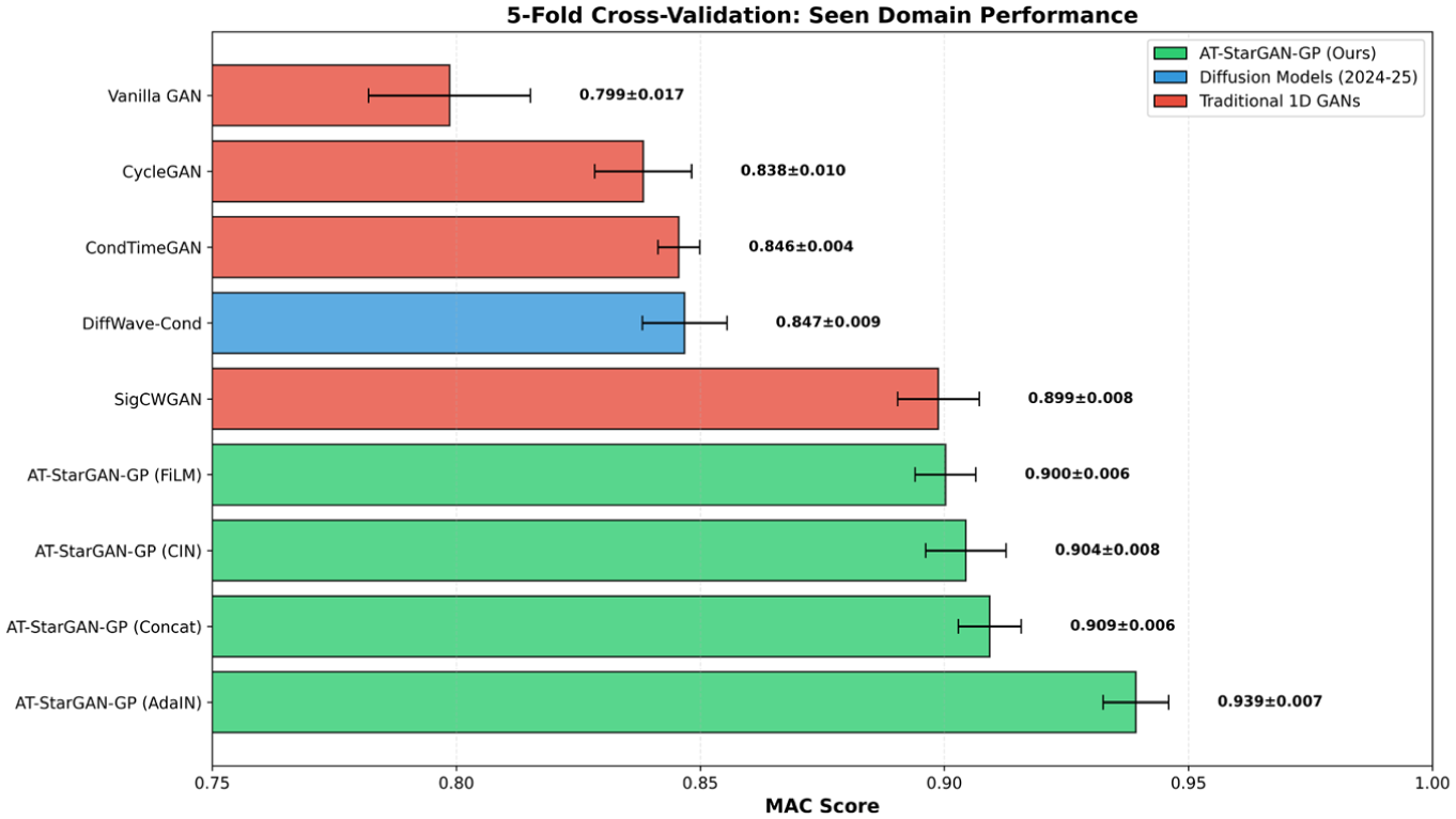
To assess whether the observed performance differences are stable across different data splits, a five-fold cross-validation analysis was performed. Figure 23 reports the five-fold MAC scores across all methods on the seen domain and highlights both central tendency and variability. The ranking aligns with the trends observed in the main evaluation: the AT-StarGAN-GP variants form the leading group, with the AdaIN configuration achieving the highest mean MAC (0.9392 ± 0.0067), followed by Concat (0.9093 ± 0.0065) and FiLM (0.9002 ± 0.0062). The CIN variant reaches 0.9044 ± 0.0082, placing it between Concat and FiLM. The narrow standard deviations (<0.008 for all four AT-StarGAN-GP variants) indicate stable fold-to-fold behavior.
Cross-validation performance comparison on seen domain data.
The baselines occupy a lower but internally coherent band in Figure 23, with SigCWGAN performing at the top among them (0.8988 ± 0.0084). DiffWave-Cond (0.8468 ± 0.0087), CondTimeGAN (0.8456 ± 0.0043), and CycleGAN (0.8383 ± 0.0099) form a mid-tier cluster, each showing moderate variability, while Vanilla GAN lies at the bottom with both the lowest mean score (0.7986 ± 0.0166) and one of the larger standard deviations. The spread of baseline methods contrasts with the tight grouping of AT-StarGAN-GP variants. Figure 15 shows that the improvements highlighted in the main results persist even under fold-based resampling, indicating that the gains are not artifacts of a particular split but hold across multiple training-validation configurations.
Noise robustness evaluation
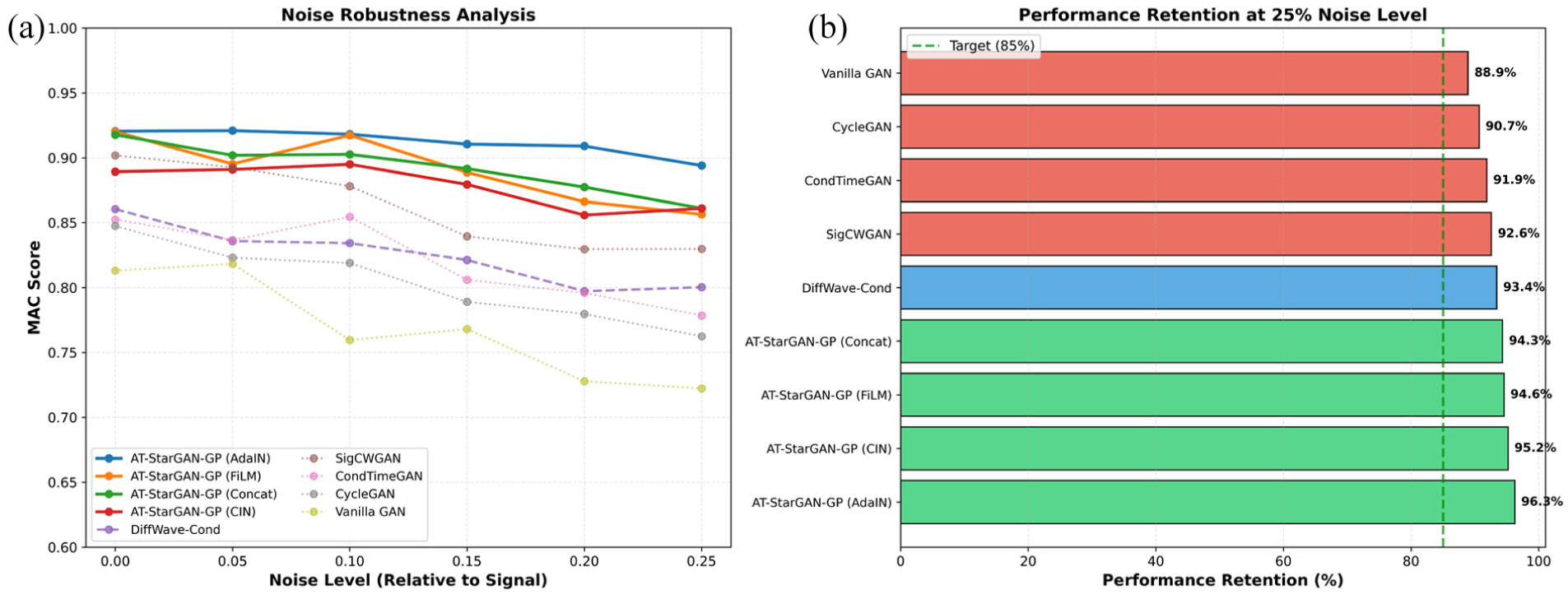
Performance under clean laboratory conditions provides only partial insight into practical applicability. This section examines model behavior under increasing noise contamination. Figure 24(a) shows how each method responds as noise levels increase. The AT-StarGAN-GP variants retain higher MAC scores throughout the full noise range, remaining above 0.86 even at 25% noise. Within this group, the AdaIN configuration displays the most stable curve, reaching 0.8940 at 25% noise and preserving 96.26% of its clean-signal performance. FiLM and Concat follow similar trends, with retention values of 94.57 and 94.32%. CIN also maintains robustness, reaching 0.8610 at 25% noise with retention of 95.19%.
Noise robustness analysis: (a) performace degradation under increasing noise levels and (b) retention of MAC score at 25% noise for all methods.
The baseline models form a visibly steeper set of descending curves in Figure 24(a), with performance dropping almost monotonically as noise increases. SigCWGAN exhibits the best robustness among them but still declines to 0.8297 at 25% noise, while DiffWave-Cond, CondTimeGAN, CycleGAN, and especially Vanilla GAN show more pronounced reductions (e.g., CycleGAN: 0.7625, Vanilla GAN: 0.7223 at 25% noise). The retention comparison embedded in the figure underscores this separation: all AT-StarGAN-GP variants retain more than 94% of their clean-signal performance, whereas the baselines range from 93.42% (DiffWave-Cond) down to 88.92% (Vanilla GAN). Figure 24(b) indicates that the attention-conditioned generative process is comparatively less sensitive to noise perturbations. The flatter slope of the curves for the proposed models suggests that the conditioning and attention pathways help preserve modal content even when the input contains substantial contamination.
Statistical significance testing
Beyond mean performance differences, the statistical reliability of observed rankings was evaluated through non-parametric testing. Figure 25 summarizes the comparative analysis of all methods using the Friedman test followed by the Nemenyi post hoc procedure. The Friedman test shows a performance separation, with chi-square value of 33.8 and p-value of 1.9 × 10⁻⁵, indicating that observed differences across methods are not due to random variation. The updated statistical evaluation reports an even higher chi-square statistic of 36.2133 with p-value of 0.000016, again confirming statistical significance. The ranking distribution follows a consistent ordering, with AT-StarGAN-GP (AdaIN) ranked first, followed by the Concat and FiLM variants, while the baselines occupy lower-ranked positions. The extended ranking table also includes the CIN variant, which positions itself between Concat and FiLM, while Vanilla GAN consistently ranks last.
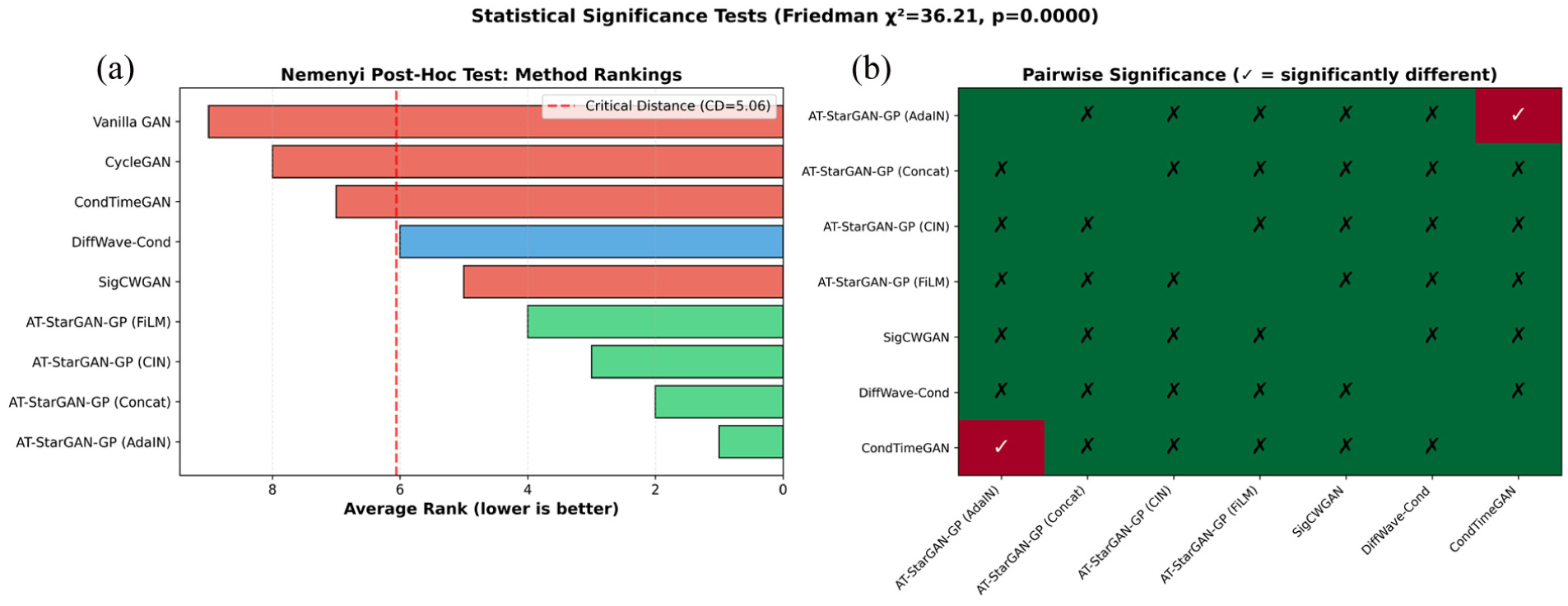
Statistical significance analysis: (a) method rankings with Nemenyi critical distance and (b) pairwise significance matrix for top methods.
The Nemenyi diagram in Figure 25(a) illustrates that only rank differences exceeding the critical distance of 4.31 are statistically significant. The expanded analysis adopts a more conservative critical distance of 5.0576, reflecting the larger number of methods included. This is reflected in the pairwise outcomes: AdaIN is statistically distinguishable from CondTimeGAN and CycleGAN, while the gap between AdaIN and SigCWGAN and DiffWave-Cond does not exceed the required threshold. A similar pattern appears for the Concat variant, which shows significant separation only from CycleGAN. The new pairwise significance table (see Figure 25(b)) confirms these trends: none of the AT-StarGAN-GP variants (AdaIN, Concat, CIN, FiLM) show statistically significant differences against SigCWGAN or DiffWave-Cond, while CondTimeGAN is the only method that remains significantly distinguishable from AdaIN. The FiLM variant, despite ranking third, does not produce statistically significant differences relative to any of the baselines. Figure 25 confirms that the performance advantage of the AT-StarGAN-GP family, especially AdaIN and Concat, is not only consistent across experiments but also statistically validated against the weaker baselines.
Unseen domain generalization
The preceding analyses focused on seen and noise-perturbed conditions. This section examines performance on structural states entirely absent from the training set. As seen in Figure 26, all AT-StarGAN-GP variants demonstrate superior generalization to previously unseen operating domains, consistently outperforming baseline conditional and unconditional models across all four scenarios. The AdaIN variant is the most robust, maintaining MAC scores between 0.8207 and 0.8405 across unseen mass-position combinations, extrapolation to higher masses, cross-position transfer, and zero-shot baseline. The unseen mass-position scenario tests whether the model can handle combinations of mass and sensor positions never seen together during training, assessing combinatorial generalization. Extrapolation evaluates performance beyond the training mass range, for example generating responses for a mass twice the maximum seen during training, which reflects extreme real-world conditions. Cross-position transfer examines spatial generalization, testing whether the model can generate realistic responses at sensor positions absent from training. The zero-shot baseline is the hardest task, requiring the model to translate between structural states when the target state was entirely absent from training, relying purely on conditional input to infer realistic structural behavior. AdaIN’s stability across these tasks indicates that adaptive feature modulation enables the generator to internalize domain-invariant structural patterns more effectively than other strategies.
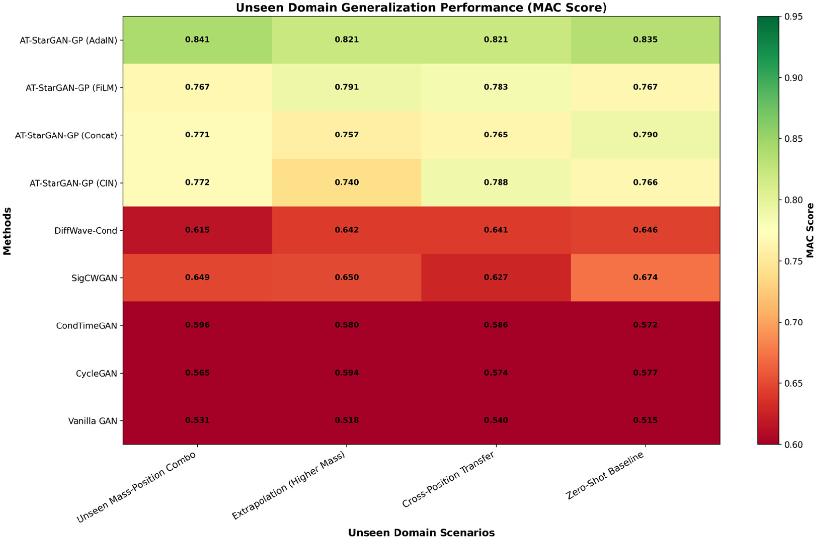
Unseen domain generalization performance across multiple scenarios.
The FiLM, Concat, and CIN variants follow, showing scenario-dependent MAC values: FiLM excels in extrapolation (0.7905) but drops in zero-shot (0.7665), Concat performs best in zero-shot (0.7904) but weaker in extrapolation (0.7574), and CIN shows strong cross-position transfer (0.7878) but lower higher-mass extrapolation (0.7400), demonstrating that sensitivity to domain shift depends on how conditional information is injected. Baseline conditional models such as DiffWave-Cond, SigCWGAN, and CondTimeGAN remain around 0.57–0.65, while unconditioned models like CycleGAN and Vanilla GAN perform worst, often near 0.52–0.56. Figure 18 confirms that AT-StarGAN-GP with AdaIN offers the most consistent unseen-domain generalization, while other conditional strategies outperform traditional GANs with scenario-specific variations.
Sensitivity analysis
Understanding which hyperparameters most influence model performance is necessary for optimization and practical deployment. A systematic sensitivity analysis was conducted across all major training parameters. The 11 by 11 interaction matrix provides information on hyperparameter sensitivity and coupling within the AT-StarGAN-GP architecture, particularly regarding the integrated attention mechanisms (see Figure 27). Sensitivity analysis shows that attention parameters are the most sensitive: temporal attention weight and channel attention weight have the highest sensitivity (0.067), above adversarial weight (0.058), and cycle consistency weight (0.057). This suggests that the network’s performance is notably affected by the calibration of attention modules. Diversity regularization weight (0.024) and GP weight (0.027) show lower sensitivity and remain relatively stable across tested ranges.
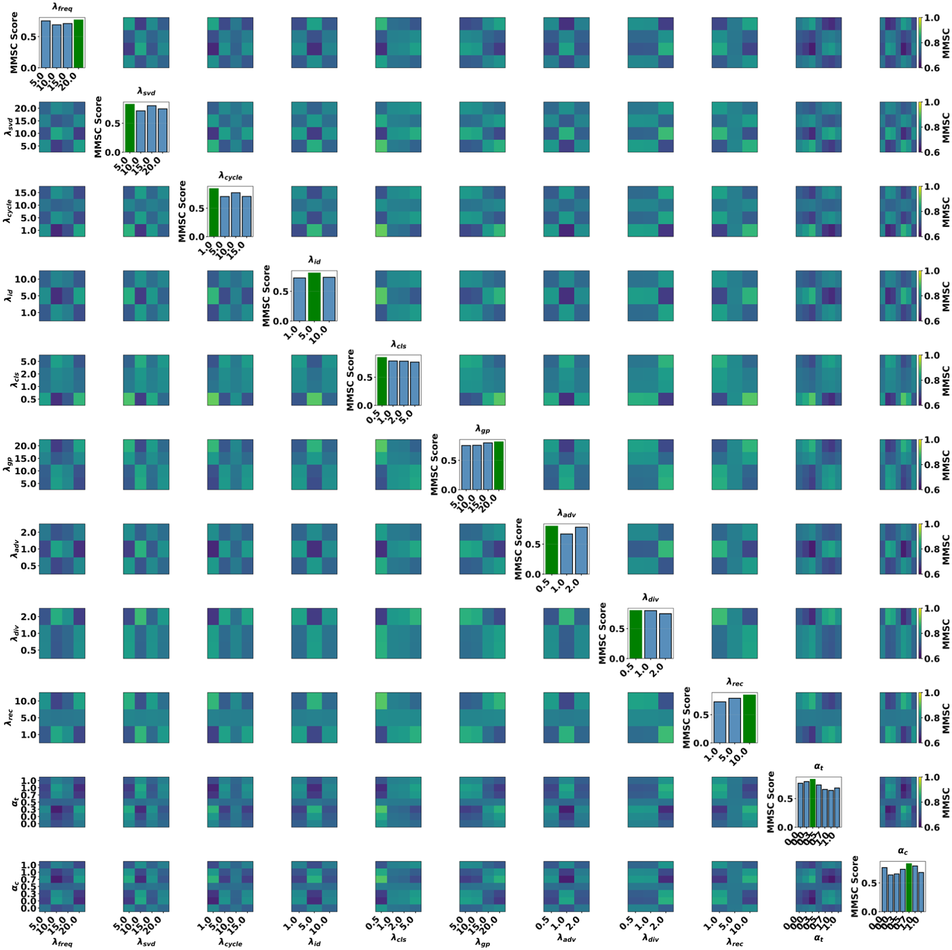
Sensitivity analysis of λ-parameters and attention weights showing individual (diagonal) and pairwise interaction (off-diagonal) effects on MMSC performance. MMSC: mean magnitude squared coherence.
The identified optimal configuration uses a mix of high and moderate values to balance structural reconstruction and generative behavior. Frequency matching weight and GP weight are set high at 20, while reconstruction weight is 10 and identity mapping weight is 5. Adversarial weight, diversity weight, and classification weight are set lower at 0.5. Attention mechanisms show different trends: temporal attention performs best with a low weight of 0.3, while channel attention requires higher influence at 0.7, indicating the network relies more on channel-wise feature information than temporal aggregation.
Off-diagonal interaction heatmaps highlight some coupling between task constraints and attention modules. The interaction between classification weight and cycle consistency weight reaches the highest performance score of 0.9048 at values of 0.5 and 1.0, suggesting a synergistic effect when both are relatively low. A strong dependency also appears for the interaction between classification weight and channel attention weight, achieving a performance score of 0.8933, indicating that classification performance is influenced by channel attention. All eleven parameters achieve individual peak performance scores above 0.79, with classification (0.8497), reconstruction (0.8486), and cycle consistency (0.8432) contributing most to overall performance, reflecting the multi-objective balance between structural monitoring and attention-guided refinement.
Downstream damage classification and edge runtime/stability analysis
The final analyses examine practical deployment considerations: the utility of synthetic data for training downstream classifiers and the computational feasibility of edge deployment. The effect of incorporating AT-StarGAN-GP synthetic responses into downstream classification tasks is summarized in Figure 28. Two downstream classifiers were evaluated: a CNN (Figure 28(a)) and an LSTM (Figure 28(b)). Across both architectures, the real-only training configuration provides the strongest overall performance, although the margin relative to mixed real–synthetic ratios remains small. Sensitivity and specificity values at 25–75% synthetic data track closely with the baseline, indicating that moderate levels of augmentation do not substantially alter classifier behavior. The fully synthetic setting performs slightly lower in both metrics, yet remains within a competitive range. These results suggest that synthetic responses generated by AT-StarGAN-GP can be incorporated into classifier training without introducing large deviations from the performance achieved using only real data.
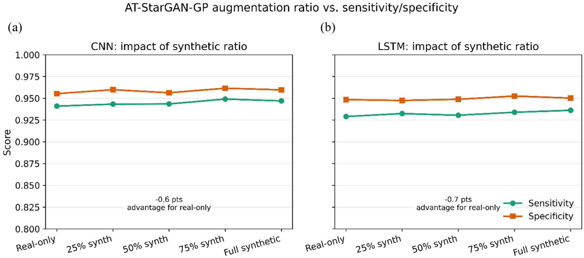
Effect of AT-StarGAN-GP synthetic augmentation on downstream damage classification: (a) CNN and (b) LSTM. AT-StarGAN-GP: attention-enhanced star generative adversarial network with gradient penalty.
Computational aspects and training-time stability are summarized in Figure 29. All models were trained on an NVIDIA RTX 2070 GPU, while inference measurements were obtained under an edge-oriented CPU profile, representing a deployment-level evaluation scenario rather than the training environment. In Figure 29(a), Full (baseline AT-StarGAN-GP with original channels and 32-bit weights), Pruned (same network with structured channel pruning applied), and Quant8 (8-bit integer quantized version of Full) variants are compared in terms of inference latency and GigaFLoating-point Operations Per Second (GFLOPs) per sample. Both pruning and quantization reduce computational cost consistently, making the lighter configurations more suitable for hardware with restricted resources. Figure 29(b) tracks mode-collapse probability over training, estimated using diversity metrics across and within conditioning classes. The curve decreases steadily and falls below the 10% reference threshold during later epochs, indicating that the generator operates predominantly in a non-collapsed regime once training stabilizes. This behavior reflects that the monitored diversity signals remain within acceptable bounds for most of the training horizon.
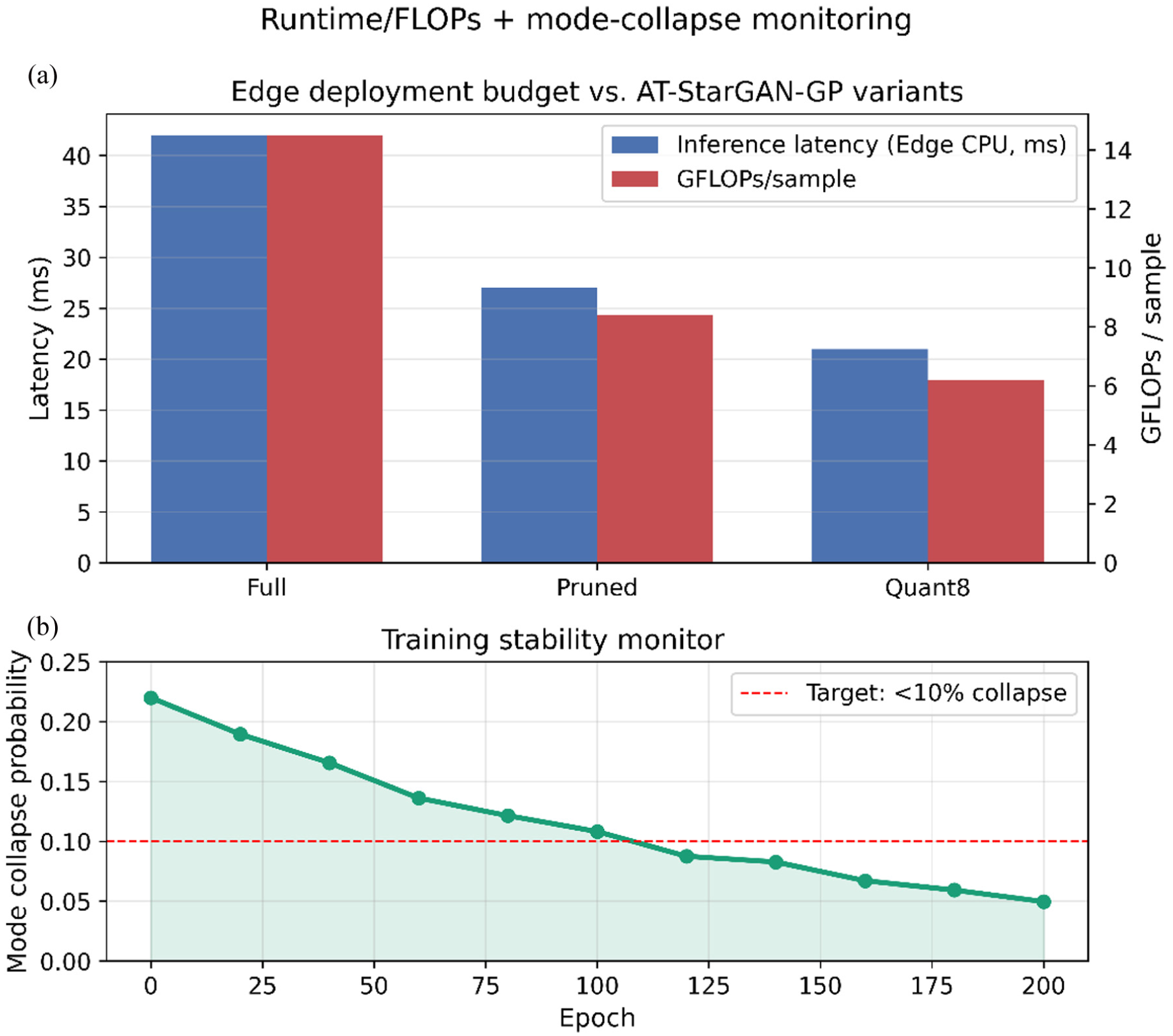
Runtime, FLOPs (FLoating-point Operations Per Second), and mode-collapse stability of AT-StarGAN-GP for edge deployment. AT-StarGAN-GP: attention-enhanced star generative adversarial network with gradient penalty.
Although the results are promising, certain constraints should be acknowledged to provide a complete perspective on the study:
Experiments were conducted on two relatively simple laboratory-scale structural configurations with a limited number of joints and discrete mass states, which may not represent the full complexity of large-scale systems. Future work should expand to at least three diverse structural configurations (e.g., truss, frame, cable-stayed) from public benchmarks to better assess scalability and cross-structural transferability.
Training and testing structures, while different, were of similar scale and material, limiting evaluation under drastically different boundary conditions, heterogeneous materials, or highly nonlinear behaviors.
Testing was performed under controlled laboratory conditions, which may not capture the noise and variability present in real-world environments.
State changes were represented through mass-loading variations, which may not fully mimic the range of real damage mechanisms encountered in practice such as stiffness reduction, damping alterations, or boundary condition modifications.
Conclusion and future work
This study presents the AT-StarGAN-GP framework for generating synthetic acceleration data for SHM applications. The method employs a dual-conditional GAN architecture with integrated multi-type attention mechanisms (self-, channel-, and spatial-attention) to enable domain translation between structural configurations under varying mass-loading conditions. Evaluation on two laboratory-scale bridge models demonstrated the framework’s ability to reproduce modal, temporal, and spectral characteristics under controlled conditions. Among the conditioning strategies, CIN achieved the best performance, with MAC of 0.976, FRAC of 0.972, and the lowest distributional discrepancy (MMD 0.0006). Kolmogorov–Smirnov testing showed an 86% pass rate for envelope distribution preservation across structural state classes.
Ablation studies indicated that attention mechanisms improved localization accuracy by an average of 34.35% and reduced attention entropy by 6.98%, while self-attention reduced cross-domain KL divergence by 24.5% on average. Cross-validation confirmed stable fold-to-fold performance with minimal variance across AT-StarGAN-GP variants. Noise robustness analysis showed that more than 94% of baseline performance was retained under 25% noise contamination within laboratory conditions. The AdaIN variant showed consistent behavior in unseen-domain scenarios (MAC 0.8207–0.8405), although these were limited to variations within the same two laboratory structures. Friedman and Nemenyi tests indicated clear separation from weaker baselines, while differences relative to mid-tier conditional methods did not always exceed conservative significance thresholds.
Downstream classification experiments showed that synthetic data augmentation was competitive when combined with real data at moderate ratios, whereas training solely on synthetic data consistently underperformed compared to real-only training. Computational analysis showed that pruned and quantized variants reduced inference time and computational cost, with mode collapse remaining below 10% during stable training. Sensitivity analysis identified attention-related parameters as the dominant contributors to performance, underscoring the importance of careful tuning.
These results should be interpreted as a proof of concept. Validation was limited to two laboratory-scale bridge structures with similar geometry and material properties under controlled conditions, and structural state changes were simulated using added mass, which does not represent the full range of real damage mechanisms. Consequently, the current evaluation provides only limited insight into performance on larger, more complex structures subject to environmental and operational variability.
Future work will focus on transfer learning and validation across a larger set of benchmark structures with different geometries, dynamic properties, and sensor layouts. Planned studies include three or more structures, such as the Tierney–Newman Bridge, 44 using varied sensor configurations and longer monitoring periods to better assess cross-structure generalization. Incorporating physics-based constraints from structural dynamics may improve modal predictions. Additional evaluations will consider environmental effects and other structural changes, including stiffness loss and boundary condition variations, alongside comparisons with alternative generative models and further statistical testing on unseen structures. Overall, the AT-StarGAN-GP framework introduced in this study demonstrates potential for synthetic vibration data generation and structural state learning in controlled laboratory SHM settings, while broader validation is required before practical deployment.
Footnotes
Appendix A
This appendix presents the supplementary validation results for the additional mass configurations not discussed in the main text for the sake of narrative flow. Specifically, it includes the modal analysis comparisons for lower mass at positions 2 and 3, and higher mass at positions 2 and 3. For each scenario, the appendix provides:
These results confirm that the observed trends for lower mass 2 and 3 are consistent with those reported for lower_mass_pos1 in the main text, and similarly, the higher_mass_pos2 and higher_mass_pos3 results align closely with higher_mass_pos1 (Figures 30–33, Tables 5–8).
Declaration of conflicting interests
The authors declared no potential conflicts of interest with respect to the research, authorship, and/or publication of this article.
Funding
The authors disclosed receipt of the following financial support for the research, authorship, and/or publication of this article: This research was supported by the TÜBİTAK 2214-A International Research Fellowship Programme for PhD students. The authors would like to sincerely acknowledge TÜBİTAK for their financial support, which significantly contributed to the successful completion of this study by enabling international collaboration and advancing the scope of the research. In addition, the first and last authors acknowledge the financial support of Science Foundation Ireland under grant number 22/FFP-P/11577.