
Abstract
This paper aims to assess the influence of stiffeners and sensor transfer functions on the measurability of acoustic emission (AE) waves in ship structures travelling as ultrasonic-guided waves. A procedure for evaluating this influence by calculating sensor correction coefficients has been developed. After applying the obtained correction coefficients, the transmission of the ultrasonic-guided waves and their dependence on the angle of incidence and different frequency content are investigated using finite element simulations and experimental measurements. The experiments examine the propagation of 60 and 150 kHz AE signals in a 10-mm thick steel plate. By combining the results of the simulations and experimental results, the attenuation due to the presence of stiffeners turns out to be less than 5 dB and the transmission coefficient appears to have limited variation for different angles of incidence. The results of this study can be used to optimize the accuracy and coverage of AE monitoring systems.
Keywords
Introduction
Ships are structures that operate in corrosive environments are subjected to highly variable dynamic loads. Fatigue and corrosion damage can develop in these structures, compromising their structural integrity and residual life.1–3 In particular, the ship hull structure consists of stiffened panels which form a structural frame of transverse and longitudinal elements. Intersections between transversal and longitudinal stiffeners and welded joints are the areas where fatigue-induced cracks may most likely develop. As a consequence, damage that builds in these locations can be difficult to detect and quantify.
Conventional non-destructive techniques (NDTs) that are employed to inspect ship structures are generally time-consuming, physically demanding and expensive to deploy (Figure 1). For example, magnetic particle inspection, ultrasound testing and visual inspections both manned and automated are techniques that involve periodic inspections during planned shutdowns, such as dry docking procedures.
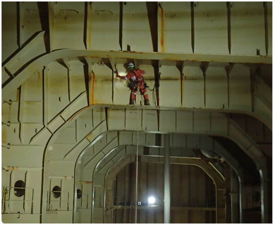
Hull inspection inside of Floating production and storage unit (FPSO) tank. 4
Structural health monitoring (SHM) systems, on the other hand, can be used to assess real-time in-service behaviour 5 differently than periodic inspections. SHM systems can be used to measure the changes in the response of structures (e.g. mechanical, electromechanical and electromagnetic) due to the occurrence of damage and translate them into information regarding the integrity status of the structures.6–9 Strain monitoring with long base strain gauges10–12 and fibre optic sensors,13,14 vibration-based monitoring with the use of accelerometers,15–17 electromechanical impedance monitoring 18 and active guided waves19–22 are examples of SHM techniques used to detect damage in ship structures.
Among the methodologies employed in SHM is also acoustic emission (AE) monitoring, which is based on the recording and analysis of transient stress waves emitted from the sudden release of energy 23 due to damage initiation and growth in the material. AE has demonstrated its effectiveness for the integrity assessment of different structures, 24 such as steel bridges,25,26 large offshore structures27–29 and pipelines.30,31 AE is suitable for thin-walled structures, such as ship hulls, as it offers the potential to cover large areas using a limited number of transducers. This passive technique, requiring no external excitation, is sensitive to the initiation and propagation of different types of damage. Its cost-effectiveness and continuous monitoring capability make it a suitable option for assessing the structural health of ship hulls and structures.
Although AE is a well-established technique within the fields of NDT and SHM, its application to stiffened ships and maritime structures has received comparatively little attention. Despite earlier attempts by industry and classification societies 32 to adopt AE, the required accuracy and reliability in quantification of damage location and activity were not consistently demonstrated to the extent required by ship operators to support their decision regarding possible maintenance actions. This is believed to be mainly due the fact that some of the complexities of the propagation of AE signals and the presence of background noise are not yet sufficiently understood or considered. In these structures, mainly ship hulls, AE waves predominantly propagate as multimodal dispersive ultrasonic-guided waves, which implies that different modes exhibit distinct sensitivities as well as different dispersion and attenuation behaviours. In addition, structural elements such as stiffeners give rise to wave scatterings and reflections, directional variability and mode conversions, which increase waveform complexity and make the interpretation and localization subjected to larger uncertainties. When combined with the non-stationary operational background noise, the factors have contributed to the limited use of AE for stiffened ship structures to date. For accurate fatigue crack detection using AE, it is critical to understanding how ultrasonic-guided waves interact with structural members and how the damage detection limit may be affected by these interactions. Furthermore, typical AE sensors are resonant-type piezoelectric transducers, notably influencing the shape and amplitude of the AE signals. The present work considers these complexities by analysing stiffener-induced attenuation and sensor-specific variability, and by introducing corrective measures to support more reliable AE monitoring in maritime environments.
It is noted that the way AE is viewed in this research as passive guided waves has similarities but also key differences with the active guided waves, which are well-established for inspection of pipelines. In AE, the source guided waves are generated by damage growth, while in active guided waves the source is a controlled external pulse. Past research on active guided waves and their interactions with structural elements such as stiffeners provided valuable insights,33–35 nevertheless there remains a lack of comprehensive methodologies for assessing AE. In this context the desire is to maximize the coverage of the monitoring system. This is particularly related to the transmission of guided waves through stiffened steel plates across the frequency ranges and angles of incidence relevant to resonant transducers used in AE monitoring applications. However, maximizing the coverage presents several challenges, such as determining the transmission coefficients in the presence of welds and handling resonant sensors with large amplitude variation over narrow frequency bands. As an example, resonant sensors of the same type can exhibit transfer-function variability, which can potentially have influences much larger than the influence of stiffeners, making it necessary to account for this variability first.
The novelty of the present study lies therefore in the assessment of the influence of welded stiffeners in AE monitoring of maritime structures and in the development of a methodology to correct for sensor transfer-function variability. In combination, these aspects address a critical gap in the existing literature, where the joint influence of stiffeners and sensor variability on AE wave propagation has not yet been systematically examined.
In earlier work by the author, 36 the influence of stiffeners on guided-wave propagation was investigated in limited conditions, and it was recognized that correction factors for the sensor transfer functions are necessary. The present study builds upon that preliminary investigation by introducing a methodology to account for such correction factors, and by extending the analysis to additional excitation frequencies and scenarios not previously examined. The objective is to investigate the propagation of fundamental guided-wave modes for different frequencies representative of damage sources to AE sensors, analysing wave interactions with structural elements while accounting for the influence of sensor transfer functions on measured AE signals. The fundamental guided-wave modes are considered in this study since most of the energy is carried by such modes in the propagation of AE signals.
Firstly, an algorithm is developed to determine the amplitude corrections for the resonant-type sensor transfer functions, addressing a key challenge in accurate wave measurement. Subsequently, an analytical formulation for the transmission coefficient of waves through a stiffener is derived, contributing to the theoretical understanding of wave-structure interactions. Through an integrated experimental and numerical approach, wave transmission coefficients are computed across different frequencies and angles. This comprehensive analysis incorporates the sensor corrections into the experimental measurements and accounts for the complex effect of welds.
In the second section, the methodology will be presented. The third section will outline the details of the numerical simulation while the fourth section will discuss the specifics of the experimental setup. The fifth section will present the results and discussions and the seventh section will provide the conclusions.
Methodology
Fatigue and corrosion damage in steel emit signals during their evolution predominantly recorded in the range of 50–450 kHz. 37 In ship structures, consisting of thin-walled components with thicknesses typically in the range of a few millimetres to a couple of dozen of millimetres, such damage-induced AE signals generally propagate as multimodal dispersive ultrasonic-guided waves. 7 To describe these AE waves mathematically in the frequency domain, the measured signal P at a sensor can be described as the convolution of the (damage-induced) source signal S with the propagation function W and the transfer function of the transducer D with the addition of a noise component N. 38 Since in this case multiple wave components propagate at the same time, the measured signal P can be expressed as the superposition of the different modes l, and with the following expression:
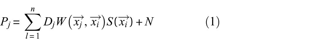
where
Accounting for the influence of sensor transfer functions
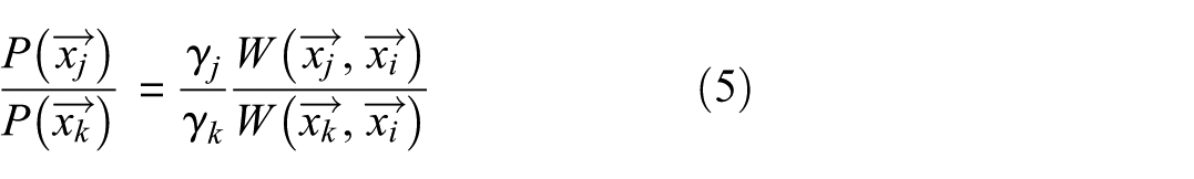
Resonant-type AE sensors inherently alter the amplitude and frequency content of the detected signals due to their transfer-function characteristics. To account for the influence of the sensor transfer function,
In AE monitoring it is often the fundamental wave modes that carry most of the energy. Considering one dominant wave mode and neglecting the phase difference between the transfer functions, from Equation (1) the expression of the signal measured at sensor location

To facilitate the description of the variability of sensor transfer functions, each sensor transfer function

where

Pairing Equation (4) for the same sources, the signals measured by different sensors can be related:
Combining these expressions for n sources and m different sensors, the following system of equations can be found, where the unknowns are the
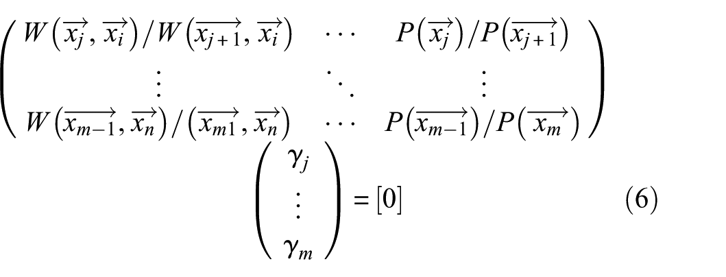
This system can be expressed in a matrix-vector format as follows:

where
As output, the vector γ containing the correction factors for each sensor is obtained. These factors are then applied to the measured AE amplitudes to take into account the influence of the sensor transfer functions. This algorithm has been performed for different source frequencies. Further implementation details regarding the solution of the system can be found in the next sections.
Transmission coefficient of stiffeners
Once the variability of the transfer function of the AE sensors is accounted for, the next step involves determining the wave transmission through stiffeners. When incoming waves hit a stiffener, part of their energy is reflected and part gets through the stiffener. Part of the energy can also be carried by converted modes after the incident, which is considered to be a contribution of smaller amplitude to the noise term in Equation (2). Figure 2 schematically shows the propagation path that an incoming damage-induced AE wave follows in a stiffened plate.
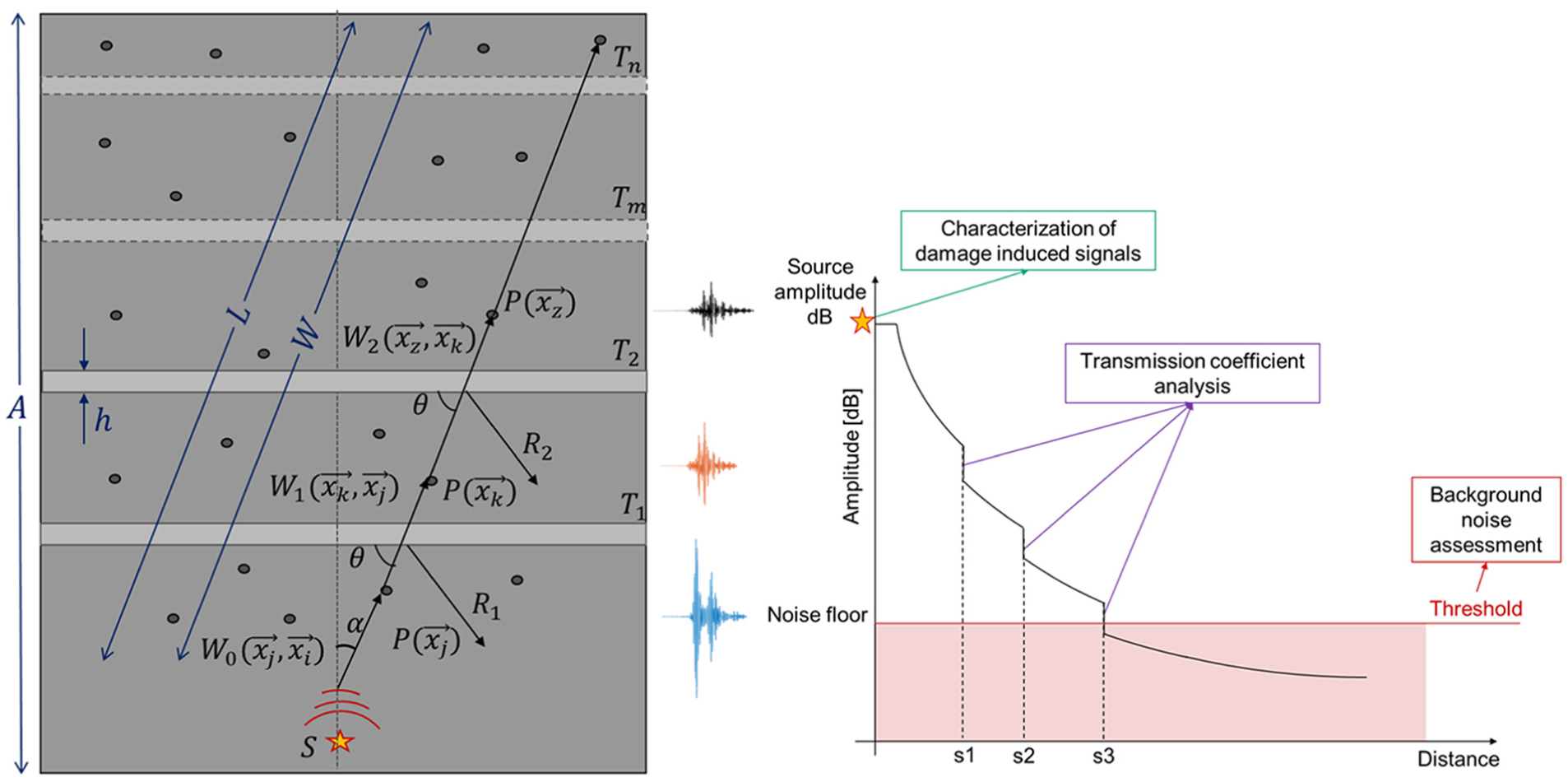
Wave propagation in stiffened steel plate of length A with multiple stiffeners of thickness h (left); damage detection in the presence of stiffeners using AE monitoring (right). AE: acoustic emission.
For an arbitrary guided-wave mode propagating in the in-plane direction of a stiffened plate and recorded with multiple sensors after the incidence with n stiffeners, Equation (2) becomes as follows:

In this expression,
Combining Equations (2) and (8), the angle-dependent transmission coefficient for a single stiffener can be described as follows:
In order to understand the influence of perturbations due to the presence of welds, the angle-dependent transmission coefficient in the logarithmic scale may be described as follows:

where
Numerical simulations
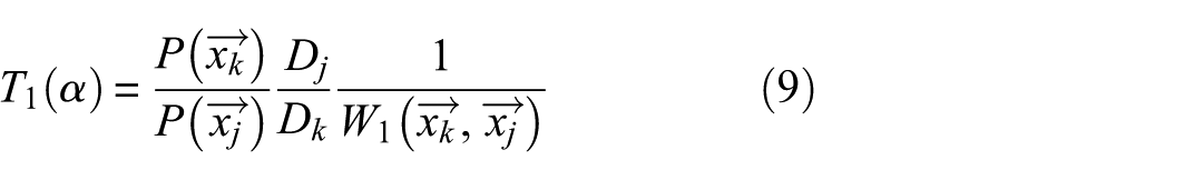
To obtain the transmission coefficient for perfectly welded joints, three-dimensional spectral finite element method (3D-SEM) simulations have been performed. The model, implemented in an in-house MATLAB code, is based on the formulation and validation of Pahlavan et al.21,39 The modelled geometry consists of a steel plate of 700 × 250 × 10 mm3 with a vertical stiffener of 10 mm thickness as shown in Figure 3. The height of the stiffener is 110 mm. The applied loading consists of a three-cycle 150 kHz pulse and a three-cycle 60 kHz pulse. Both sources have been applied in the y-direction through the thickness of the plate to excite only A0 waves. The coordinates of the source location are x = 250 mm, y = 5 mm and z = 250 mm; see Figure 3 (yellow circle). The order of the SEM basis functions in all directions is 2, the element size is 5 mm in the x and z directions and 10 mm in the y-direction. The time step for the explicit numerical time integration is 0.005 µs.
SEM model and geometry, top and side view of stiffened plate of dimensions 700 × 250 × 10 mm3. Black lines show the wave propagation directions with angles of incidence between 90 and 140°. SEM: spectral finite element method.
Four arrays of 52 transducers have been modelled on both sides of the plate and on both sides of the stiffener (blue crosses in Figure 3) to capture angles of incidence of the waves with the stiffener from 90 to 140°. The distance of the sensor arrays from the stiffener is 5 mm. A symmetry axis has been applied along the x-direction to avoid reflections from that side of the plate.
The SEM simulation duration was on average in the order of magnitude of 12 h on a standard workstation (Intel® Xeon® W-2133 CPU @ 3.60 GHz, 32 GB RAM).
Experiments
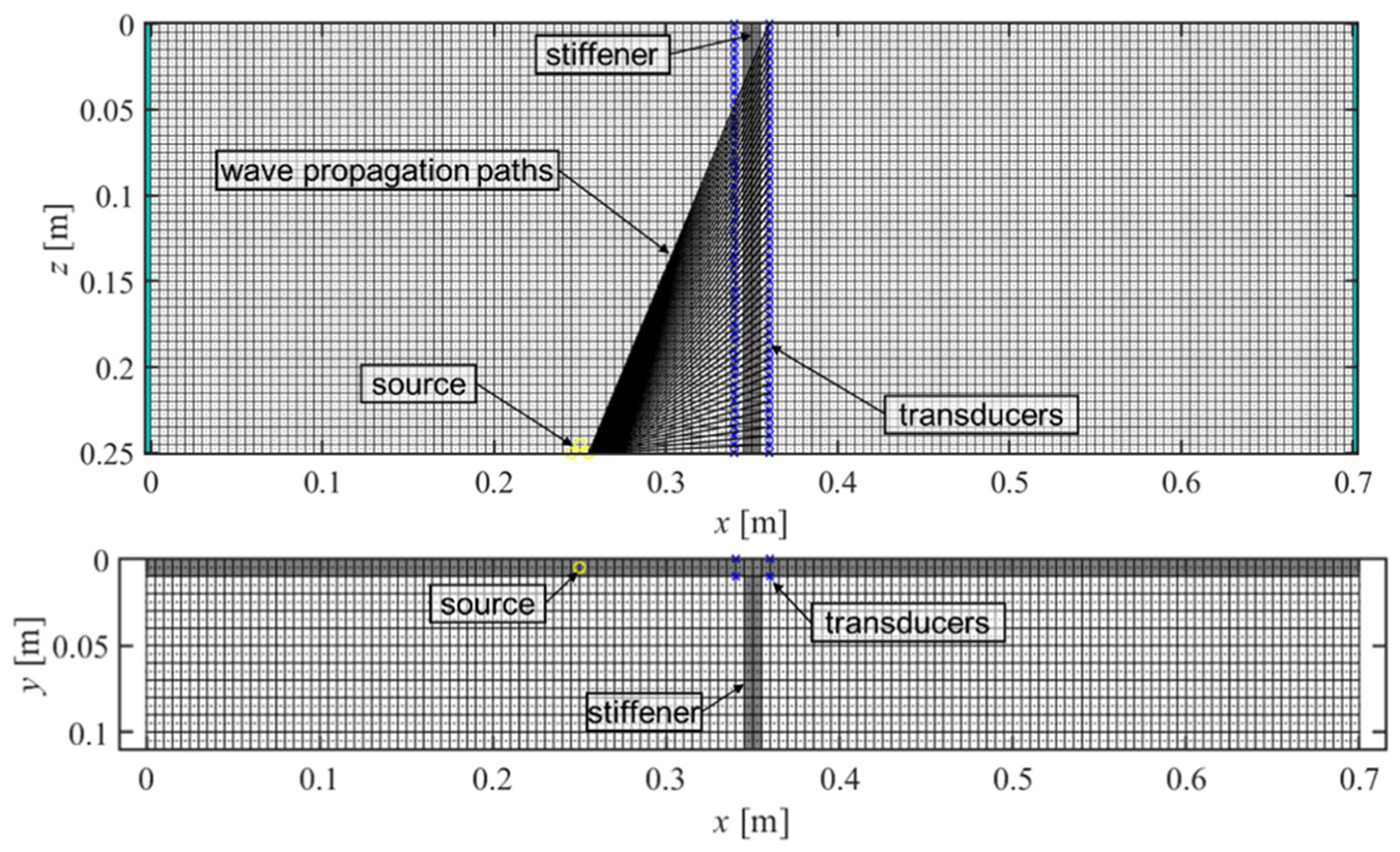
To characterize the transmission of waves through realistically welded stiffeners, experimental investigations were conducted. The experimental setup was designed to be representative of part of the inner structure of a ship. As can be observed in Figure 4, it consists of a stiffened plate. The base plate is a 1700 × 1200 × 10 mm3 S355 steel plate. The stiffener is a 7 mm thick bulb-profile, and it intersects with a longitudinal flange of 8 mm thickness. As excitations, standardized pencil lead breaks (PLBs) were performed in accordance with ASTM E976-15 to minimize the sensor influence of the measurements. At each location (1–5), 10 PLBs have been performed to ensure consistency. Pairs of R6α and R15α sensors were placed on both sides of the plate and of the stiffener (12 sensors in total, 6 on each side of the plate) to record the incoming and transmitted waves. These sensor frequencies, 60 kHz (R6α) and 150 kHz (R15α), were selected because they are considered to be representative of the range of frequencies for fatigue crack AE, 40 that is, 100–200 kHz. The transducers were connected to AEPH5 preamplifiers (40 dB), and from there to an AMSY-6 data acquisition system. The sampling frequency was 10 MHz. The acquisition was hit-based and had a rearm and duration time of 250 µs and a pre-trigger period of 400 µs. A digital band-pass filter was applied ranging from 40 to 300 kHz for both R6α and R15α sensors. This was done to ensure that lower-frequency noise was not measured. An amplitude threshold of 40 dB was applied. During the experiments, the sensors were placed in five different positions on the plate to measure waves at different incident angles with respect to the stiffener. The geometry is shown in Figure 5.

Experimental setup and instrumentation.
Sensor layout: front view (left) and side view (right).
The five receivers measuring the incoming wave ‘R11, R12, R13, R14, R15’ remained fixed throughout the duration of the experiment, to ensure cross-checking of the data. These receivers were positioned to ensure alignment with the source as it moved between locations 1 and 5, where the angles of incidence are respectively 90, 75, 65, 45 and 30°. The receiver on the other side of the stiffener is referred to as R2 in Figure 5. Like the other five receivers, this transducer was kept fixed throughout the entire experiment to ensure no variability in the results due to the coupling variation.
Results
Experimental results
For the current design, given the analysed frequencies (60 and 150 kHz) and plate thickness of 10 mm, AE ultrasonic-guided waves propagate in two distinct wave modes: the fundamental symmetric wave mode S0 and the fundamental antisymmetric wave mode A0. 7 Throughout the analysis of the experimental data, it was observed that the utilized piezoelectric sensors are most sensitive to the out-of-plane displacement, meaning that the first antisymmetric wave mode A0 can be considered the predominant one captured by the sensors. The S0 mode was only visible in isolated cases, with amplitudes significantly lower than A0, and could not be reliably analysed across the different sensors and configurations. For this reason, the amplitude of the A0 mode has been further analysed for both the experimental and numerical investigations and for both considered frequencies.
The frequencies of 60 and 150 kHz were selected for the analysis because they fall within the range associated with fatigue crack AE signals. For this reason, they are also the most-widely used frequencies in industrial applications of AE for fatigue damage. Since the excitation was generated through PLBs with a reasonably flat frequency spectrum, the actual frequency content recorded is primarily governed by the sensor transfer function. For consistency, the same frequencies were adopted in the SEM simulations.
The raw data (see as example waveforms and their Fast Fourier Transform (FFT) in Figures 6 and 7) was processed using a band-pass filter with frequency ranges of [40, 80] and [110, 180] kHz for the 60 and 150 kHz test cases, respectively. This filtering approach isolated the sensors’ response within the targeted frequency bands while attenuating extraneous spectral components outside these ranges. Results are shown in Figure 8, where the normalized waveforms are plotted according to their arrival times and reciprocal distances with respect to the source.
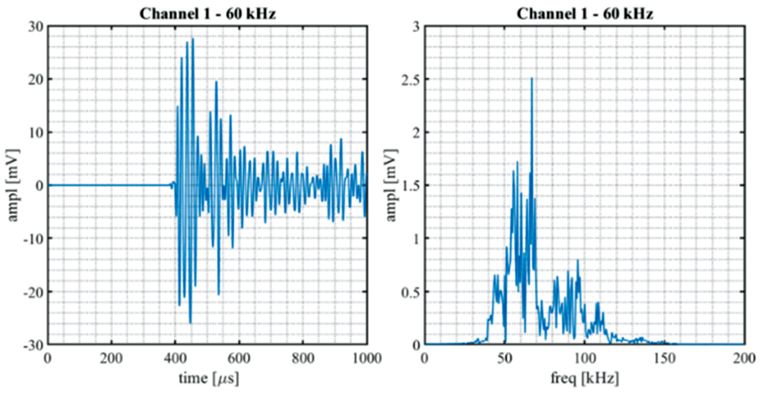
Waveform and FFT from experimental raw data for 60 kHz case.
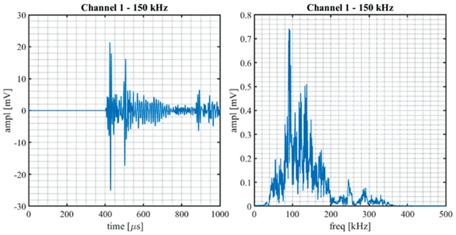
Waveform and FFT from experimental raw data for 150 kHz case.
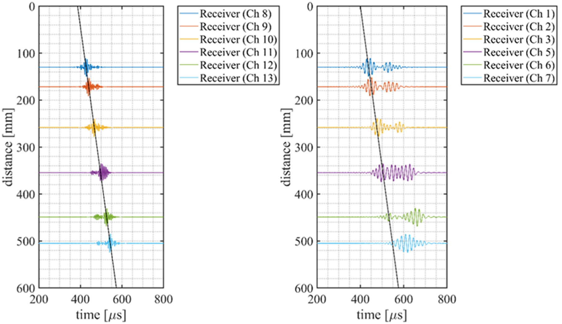
Identification of A0 wave mode amplitudes, 150 kHz (left) and 60 kHz (right).
In both the experimental and SEM analyses, time-windowing was applied to the waveforms to isolate the first-arrival packet prior to the occurrence of boundary reflections, in order to ensure equivalent comparison between the two.
The local peak of the dominant wave mode A0 was identified for each waveform using line fitting and group speed calculations. Specifically, a straight line was fitted to connect the zero-crossing intersections with the first significant peak of each waveform. This peak identification process was automated, except for some waveforms measured by the sensors positioned after the stiffener, which needed manual correction due to wave interference effects. As shown in Figure 8, this interference with the stiffener appears to be more pronounced for the lower-frequency sensor (60 kHz). The slope of the fitted line between significant peaks indicates the propagating mode’s wave speed (see the black line in Figure 8). The angular coefficients of the fitted lines matched the theoretical group speeds of the A0 wave mode for both frequencies, which had been previously computed using the dispersion curves for a 10 mm thick steel plate (Figure 9). The values found were m = −3.14
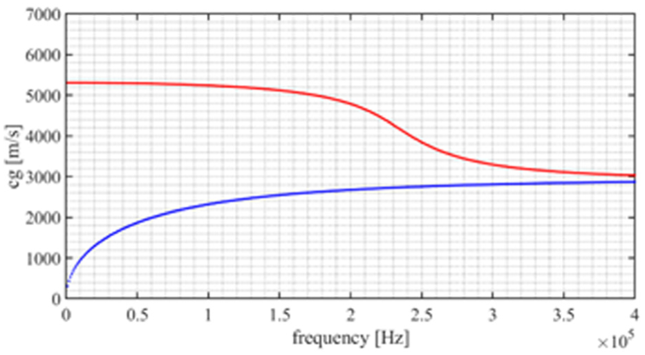
Dispersion curves for 10 mm thick steel plate (A0 mode in blue, S0 mode in red).
The material properties of the steel used in the computation of the dispersion curves are E = 200 GPa for Young’s modulus,
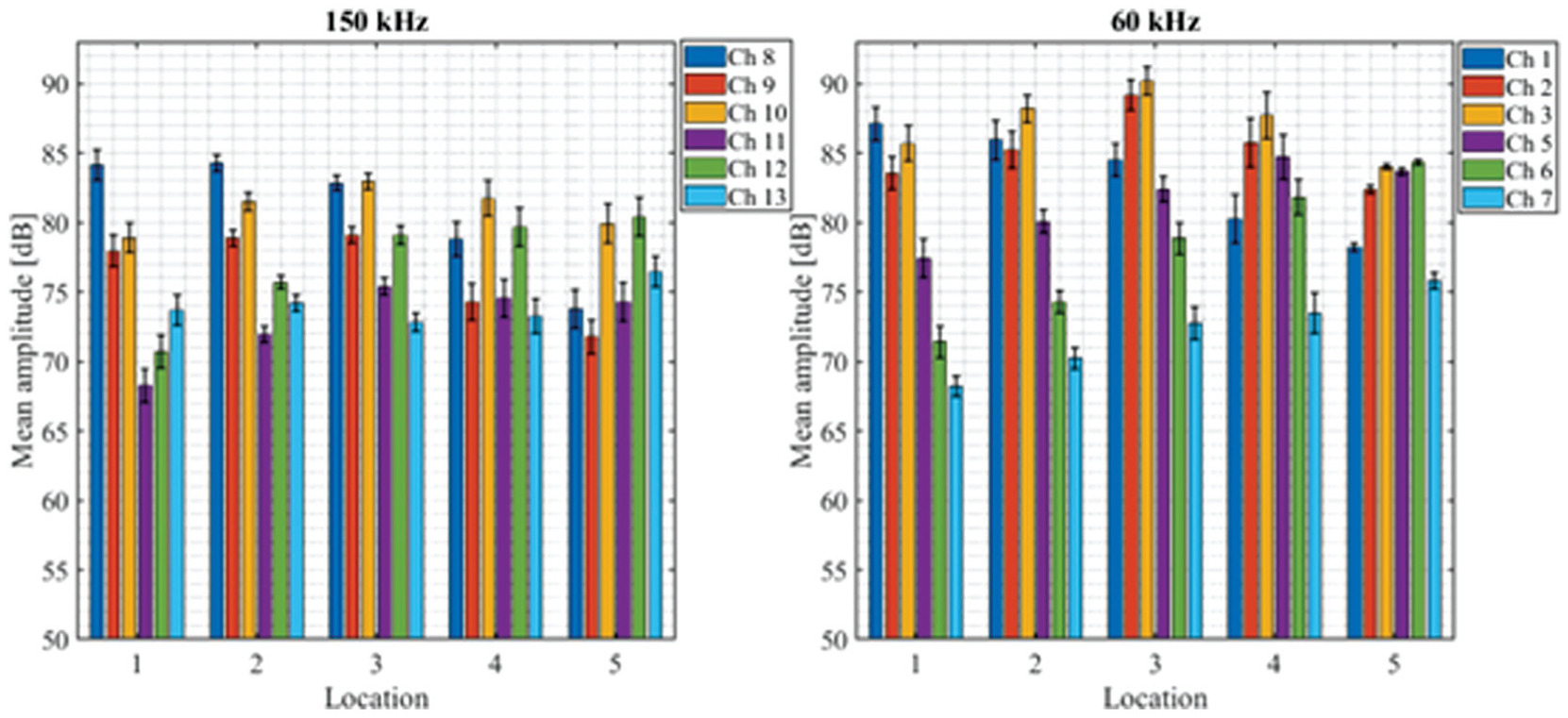
The experimental setup included transducers positioned on both the front and back sides of the plate at aligned locations. Initial analysis of the measured amplitudes for both frequencies and all channels across different source locations revealed sensitivity variations between the different sensor sets. For the 150 kHz frequency, sensors on the front side of the plate showed higher sensitivity and more consistent amplitude measurements compared to the ones on the back side of the plate. For the 60 kHz case, the back-side sensors showed higher amplitudes and better sensitivity. As a result of this analysis, for the 150 kHz case, the data set from the back side of the plate sensors (channels 1–7) was excluded, whereas data from channels 8–12, corresponding to the front side of the plate sensors, was excluded from the 60 kHz case. This was implemented based on the observed signal inconsistencies and amplitude variability that exceeded the established threshold of ±10 dB across repeated measurements. The amplitude distributions are analysed in two different ways: grouped by source location to examine the different receivers’ responses to the same source, and grouped by individual sensors to assess the amplitudes measured by each sensor across all source locations. These two perspectives provide insights into both source-location-dependent signal characteristics and individual sensor performance. Figure 10 shows the measured amplitudes for the 150 kHz case for the different source locations from 1 to 5, measured by all sensors.
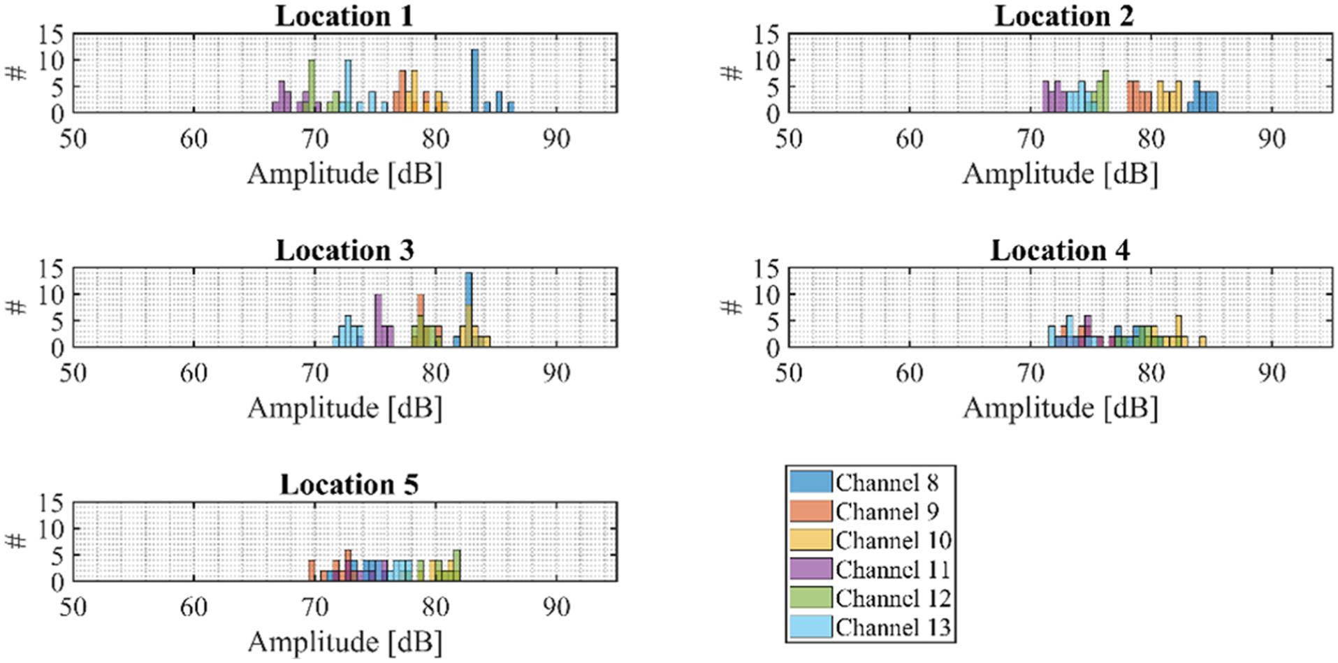
Measured amplitudes per location (150 kHz).
As expected the histogram confirms the signal attenuation behaviour of the transducers positioned on one side of the stiffener, demonstrating a consistent amplitude decay rate which aligns with the theoretical wavefront propagation model. The recorded amplitudes are in the range of 70–85 dB. Channel 13 (positioned behind the stiffener) consistently shows lower amplitudes for all source locations, which is expected due to the attenuation caused by the stiffener.
Subplots in Figure 11 show the amplitudes recorded for all source locations (1–5) by the same transducer for the 150 kHz frequency. In this figure all sensors exhibited comparable amplitude detection ranges, consistently measuring signals between 70 and 85 dB across all source locations. This uniform response window suggests similar sensitivity thresholds, facilitating reliable comparative analysis between channels.
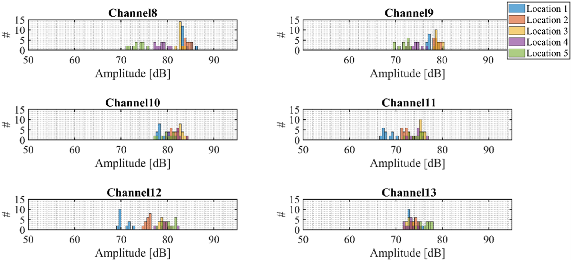
Measured amplitudes per channel (150 kHz).
Further analysis of the histogram reveals also that channel 13 consistently recorded amplitudes within a narrow range (70–80 dB) across all source locations. This small variability demonstrates the sensor’s reliability and measurement stability independent of source position.
Figure 12 shows the measured amplitudes for the 60 kHz case for the different source locations from 1 to 5, measured by all sensors. This time the range of measured amplitudes appears slightly wider than the 150 kHz sensors (70–90 dB) and the amplitudes measured at each source location are generally more uniformly distributed across channels.
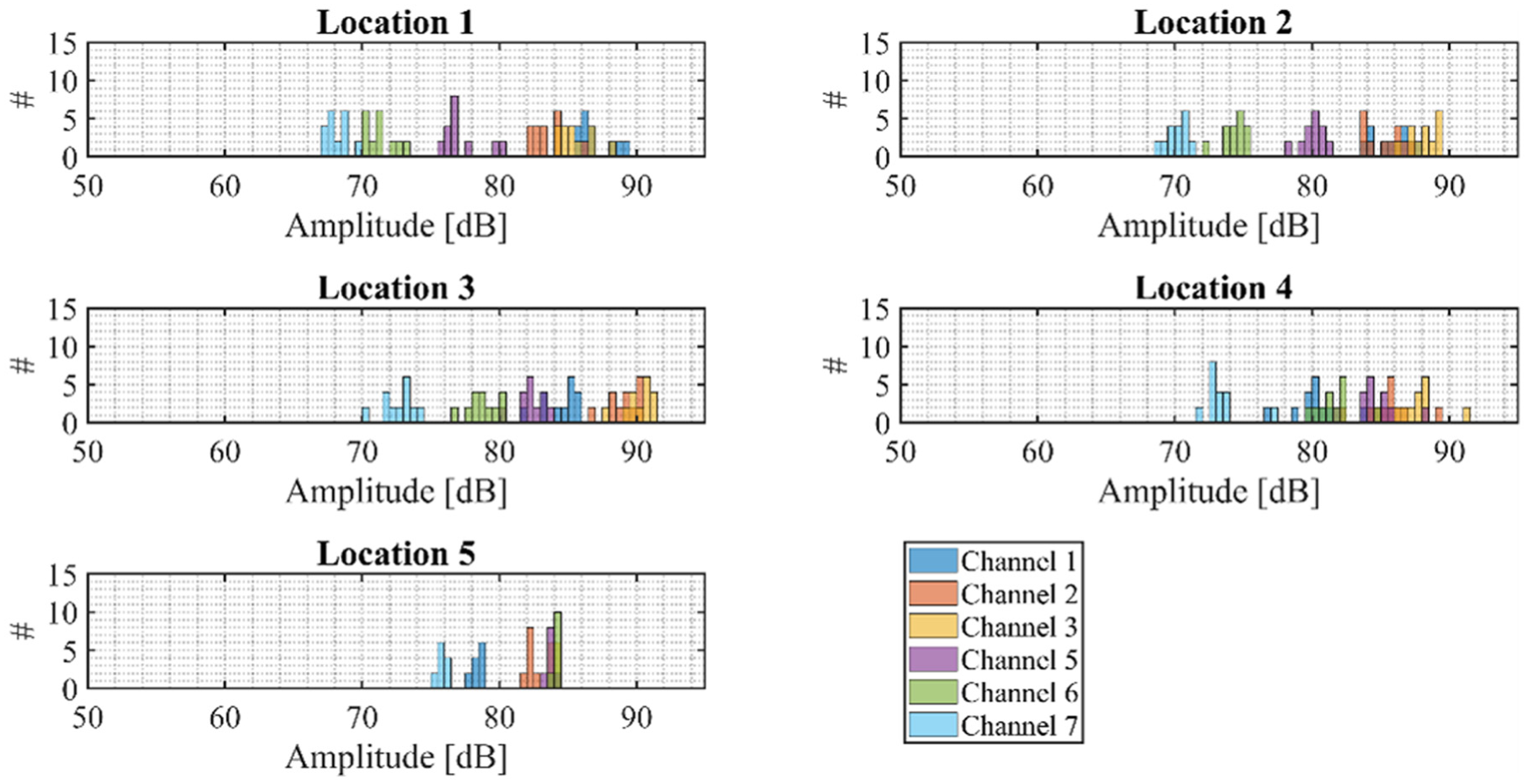
Measured amplitudes per location (60 kHz).
Figure 13 shows the amplitude distributions for channels 1–7 across the five source locations. Channels 1–5 exhibit significant amplitude peaks in the 80–90 dB range, while channels 6 and 7 show slightly lower amplitude distribution. This behaviour can be attributed to their placement relative to the stiffener: channel 7 is positioned on the opposite side of the stiffener with respect to the source locations, while channel 6 is located at a 30° angle – closest to the stiffener and most affected by its presence.

Measured average amplitudes per channel (60 kHz).
The presented amplitude values are then used as input for the equations presented in the previous section ‘Methodology’, for solving the algorithm for the sensor transfer-function corrections and for the transmission coefficient computations. More specifically, the amplitude values presented in the previous figures are substituted into the expression from Equation (4), as
Numerical simulation results
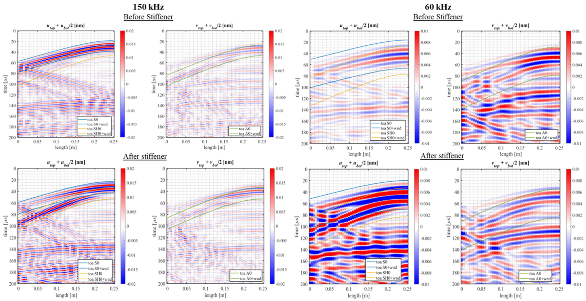
To complement the experimental observations and to better characterize the underlying wave behaviour, outputs from the 3D SEM model are discussed in this section before introducing the sensor transfer-function correction procedure and the transmission coefficient analysis. To compare with the experimental conditions, with sensors that were predominantly sensitive to out-of-plane motion, the numerical simulations were first performed using an A0-only excitation. Figure 14 shows the B-scans for the 150 and 60 kHz, the A0-only cases. These plots represent the time-distance evolution of the waves along the plate, using the in-plane u and the out-of-plane v components recorded at the top and bottom surfaces (subscripts up and bot ).
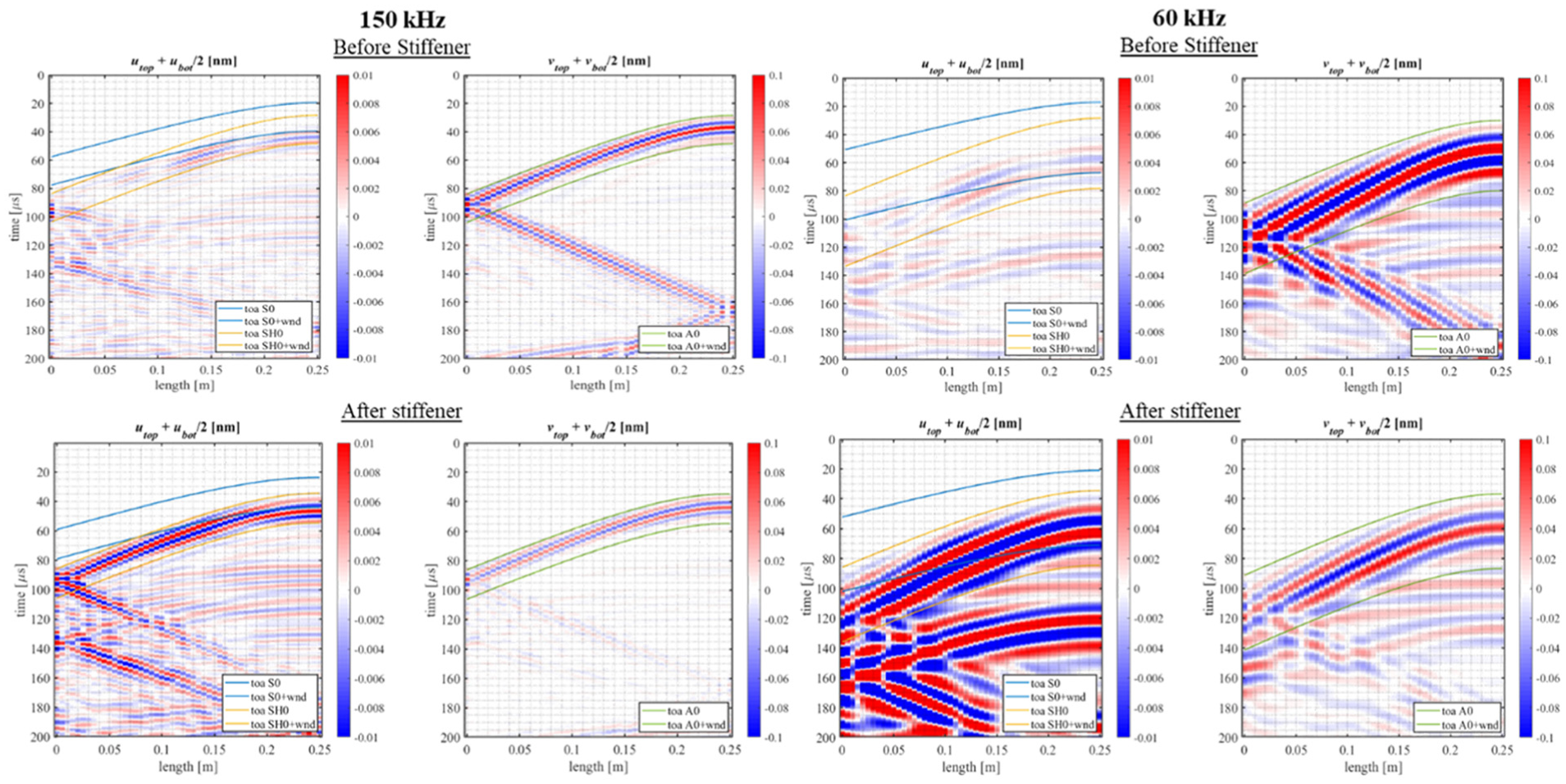
B-scan for A0-excitation at 150 and 60 kHz; before stiffener (top) and after stiffener (bottom). The solid lines show the time window bounds applied. Note the different scales, made for better visualization.
Before the stiffener, both frequencies display a single dominant wave packet corresponding to the A0 mode. After interacting with the stiffener, additional S0- and SH-wave components appear due to mode conversion, although with amplitudes notably smaller than the A0 component. The A0 mode continues past the stiffener in both cases, with increased distortion and attenuation compared with the pre-stiffener propagation.
To complement the B-scan representations with a full view of the wave motion, displacement-field snapshots at two representative time instants are presented for all three components (x and z in-plane and y out-of-plane). These snapshots provide a direct visualization of how the A0 wavefront evolves across the plate (Figure 15).
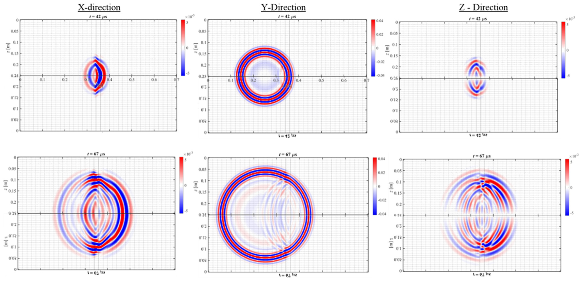
Wave propagation from A0-only excitation for 150 kHz at 42 and 67 µs. For better visualization, the displacement field has been mirrored around the symmetry line at z = 0.
The wavefield initially develops through a dominant flexural-type motion, consistent with A0-dominated behaviour. Upon interaction with the stiffener, additional displacement components (and therefore wave modes) appear in the other orthogonal directions (x and z) and propagate along and beyond the stiffener. These in-plane components arise from mode conversion at the discontinuity and are consistent with the activation of S0- and SH-type contributions. The converted components exhibit a more distorted pattern when interacting with the stiffener, whereas the original A0 wave front keeps its original circular wavefront. This behaviour is observed at both frequencies, although at 150 kHz the onset of the secondary component occurs earlier in time. For conciseness, only the displacement fields for the 150 kHz excitation are shown, as the modal evolution at 60 kHz follows the same qualitative trends.
An additional SEM simulation with S0-only excitation was performed subsequently (although not captured in the experiments). The corresponding B-scan representations illustrate the evolution of the wavefield before and after interaction with the stiffener (Figure 16).
B-scans for S0-only excitation at 60 and 150 kHz; before stiffener (top) and after stiffener (bottom). The solid lines show the time window bounds applied. Note the different scales, made for better visualization.
Prior to the stiffener, both frequencies show the expected behaviour of the S0-mode: the in-plane displacements dominate over the out-of-plane component. After interaction with the stiffener, additional scattering and mode conversion appear in the B-scans. These introduce secondary branches within the main S0 packet, and A0- and SH-type components are visible. The overall S0 wavefront remains dominant, but its shape becomes more distorted after the stiffener.
Together with the A0-only results, these S0-only simulations illustrate how the two fundamental guided-wave modes interact differently with the stiffener and how their signatures evolve across the discontinuity.
Finally, Figure 17 reports the transmission coefficients obtained from the SEM simulations for both A0-only and S0-only excitations at 150 and 60 kHz. At 150 kHz, both modes exhibit comparable transmission levels across the stiffener for the range of incidence angles considered. The S0 mode retains slightly higher amplitude than the A0 mode, which is consistent with its lower sensitivity to the local discontinuity introduced by the stiffener. Overall, transmission at this frequency is weakly dependent on the angle.
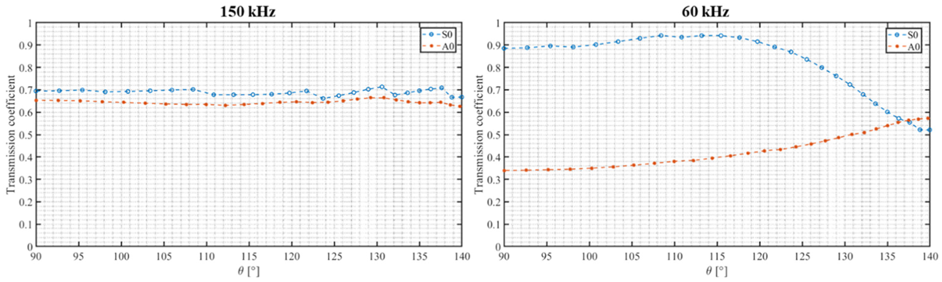
Transmission coefficients of S0 and A0 modes for 150 kHz (left) and 60 kHz (right).
For 60 kHz, the S0 mode seems to transmit more efficiently through the stiffener than A0, but its angular dependence becomes more pronounced. S0 displays higher transmission near normal incidence, followed by a progressive reduction at larger angles, likely due to stronger reflections for oblique incidence at lower frequencies. In contrast, the A0 mode remains uniformly affected around the normal angle of incidence, with an increasing transmission at larger angles.
Correction algorithm results
Through solving the system of equations presented in the methodology section as Equation (7) by substituting the amplitudes obtained from the previous analysis, the correction coefficients have been calculated. Since in this case there is a higher number of equations than unknowns, the system Equation (7) is an overdetermined system. This is because the combination of measured signals at each sensor for different sources is greater than the number of sensors. For this reason, the problem has been solved by minimizing an appropriate objective function, such as the Euclidean norm of the product between the matrix
Figures 18 and 19 show respectively the averaged measured amplitudes with their standard deviations per location for all sensors without and with the applied corrections for both the 150 and 60 kHz sensors.
Mean amplitudes per location without sensor corrections (150 kHz left side–60 kHz right side).
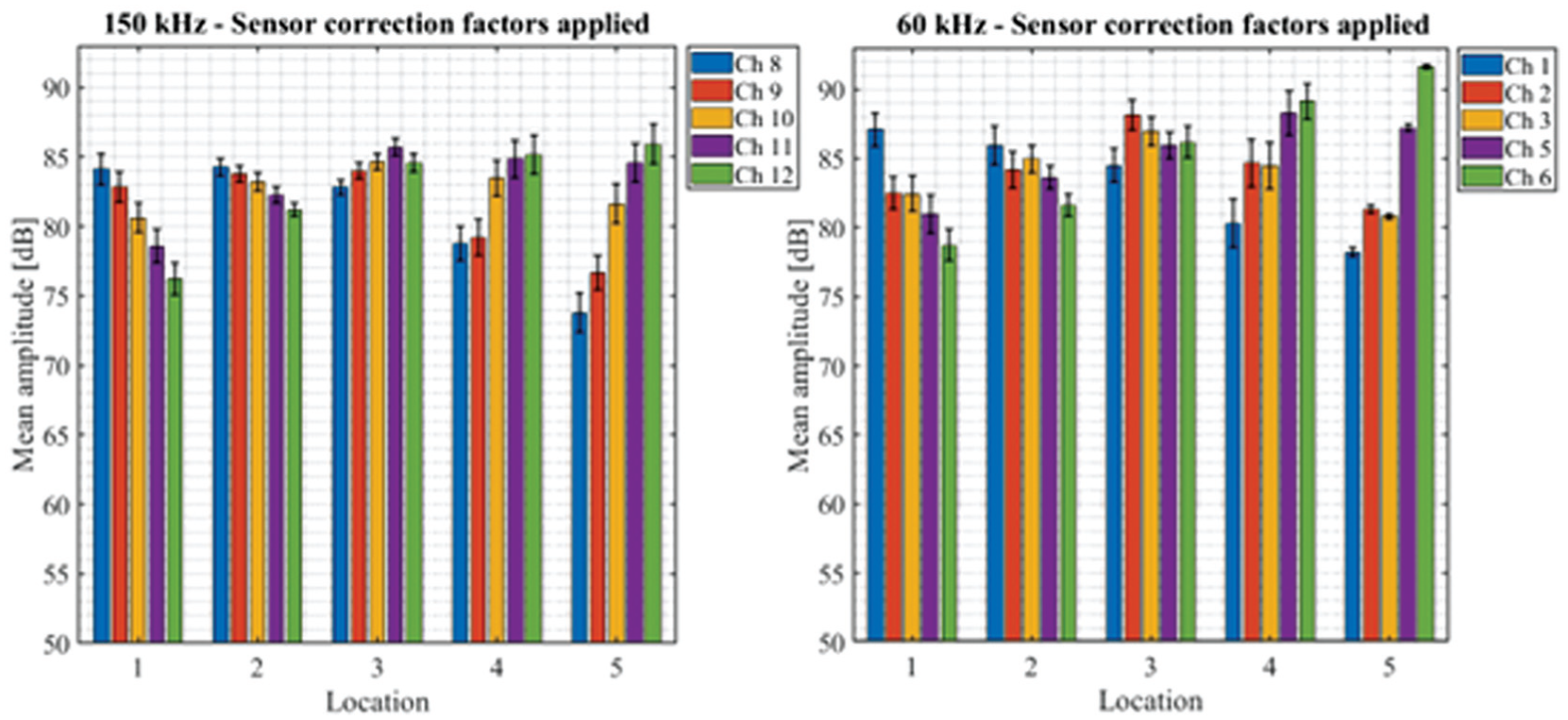
Mean amplitudes per location with sensor correction (150 kHz left side–60 kHz right side).
The algorithm shows promising and generally satisfactory results. Application of the sensor transfer-function correction tends to reduce amplitude variability across sensors and enhance the overall consistency of the recorded waveforms at both 60 and 150 kHz. Although some residual variations remain, the corrections compensate for sensor-specific sensitivity differences. As a result, the effect of physical attenuation mechanisms, including geometrical spreading decay during propagation, becomes more visible. The corrected amplitude values are subsequently employed in the computation of the experimental transmission coefficients discussed in ‘Numerical simulation results’ section.
Transmission coefficient results for A0 mode
Following the calculation of the corrected amplitudes, an analytical expression for the transmission coefficient was derived. The outputs are expressions for the transmission coefficients for different angles of incidence of the waves with respect to the stiffener and for two different frequencies (150 and 60 kHz). The experimental transmission coefficients can then be compared to the ones obtained with the numerical simulations (SEM). In this case, transmission is simply defined as the ratio between amplitude of the waves before and after the stiffener. Looking at Equation (10), the differences between the experimental values and SEM are to capture the influence of welds and associated scattering or diffraction effects on AE waves.
For the 150 kHz test case, Figure 20 shows how different the transmission values for each angle are with respect to the mean value in a dB scale. The figure includes numerical simulations and experimental results, including the ones obtained without sensor transfer-function corrections (round markers). It is promising to see that the difference in the experimental results stays within the range of ±2 dB (when including sensor corrections). The SEM results on the other side show a constant trend, indicating that there is little variation in the transmission for the different angles.
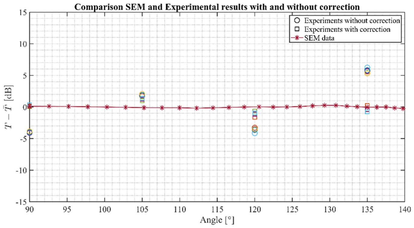
Difference in dB between transmission values and mean value for SEM and experimental data with and without sensor corrections for 150 kHz. SEM: spectral finite element method.
Understanding how the sensor correction coefficients impact the transmission coefficient results can give valuable insights on measurement artefacts introduced by the sensors themselves, the frequency-dependent sensitivity of the ultrasonic transducers and the extent to which sensor characteristics can mask or distort the signals originating from damage evolution in the material.
The differences between the experimental results and the more uniform SEM predictions are likely attributable to the weld influence, scattering and diffraction effects of the AE waves. The welding process introduces material property changes, absent in the idealized SEM model, that create angle-dependent transmission characteristics at 150 kHz. These characteristics vary along the weld length due to heterogeneous microstructure and property distributions inherent to the welding process, resulting in position-specific transmission behaviour at each angle of incidence. The SEM uniform response confirms that in an ideal scenario, transmission should remain relatively constant across incident angles, highlighting the impact of the weld. Moreover, effects of scattering and diffraction are not properly captured during the SEM simulations, explaining further the differences between the values.
For the 60 kHz test case, Figure 21 shows the difference between the transmission values for each angle and their mean value in dB scale. In this case as well, the experimental results also include the ones without sensor transfer-function corrections (round markers). Differently than the 150 kHz case, the SEM shows more variability with respect to different angles, increasing for angles different than 90°. The experimental results in this case also show a ±5 dB angular variation, slightly higher than the 150 kHz case. These frequency-dependent behaviours suggest a complex interaction between wavelength and weld characteristics. While longer wavelengths (60 kHz) are typically less sensitive to small structural details, they appear more responsive to the overall angular orientation relative to the weld and stiffener geometry. This suggests that at lower frequencies, the wavelength may interact with the weld region rather than with microscopic inhomogeneities. The higher variability in experimental measurements at 60 kHz further indicates that these interactions are more sensitive to slight positioning differences across the weld structure.
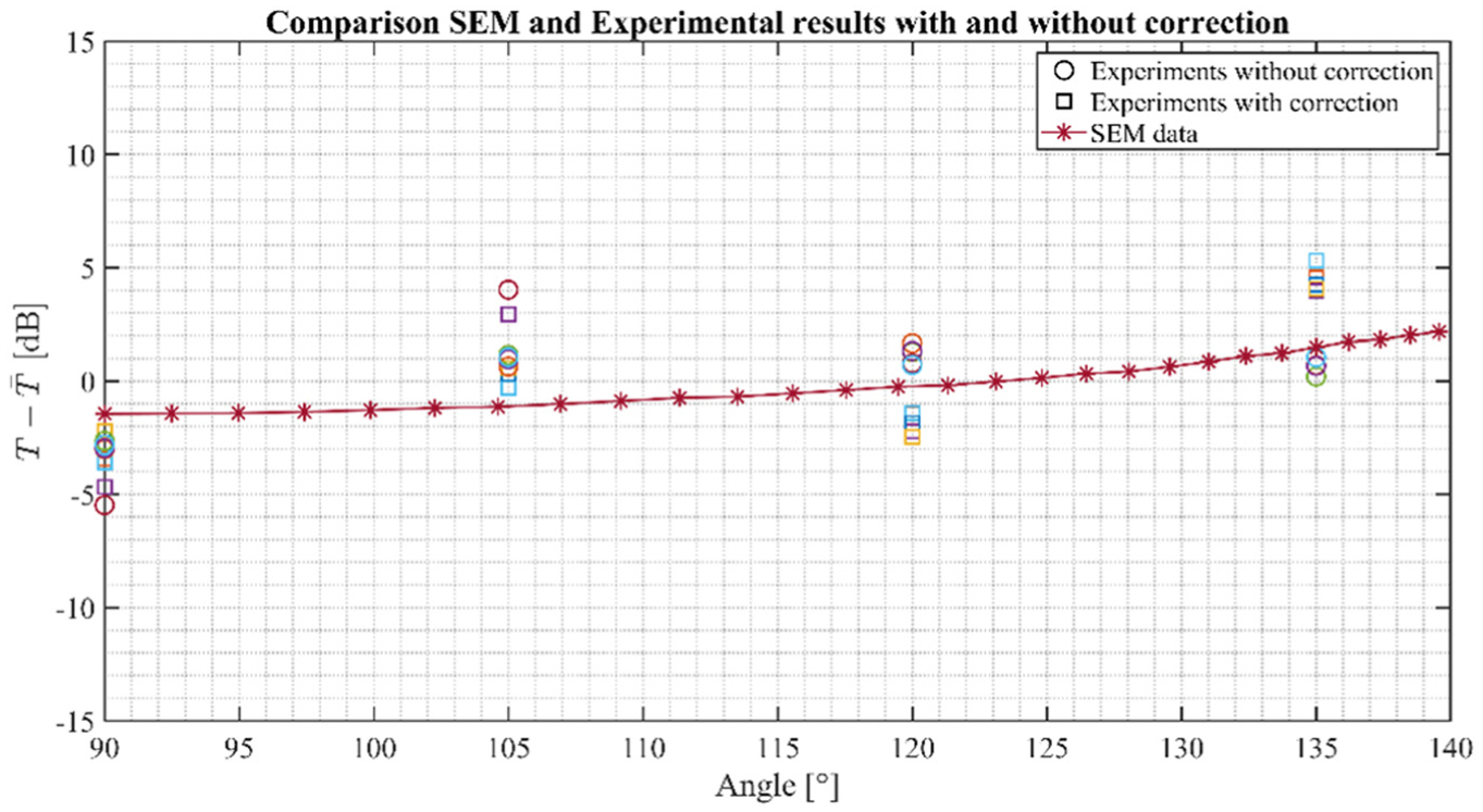
Difference in dB between transmission values and mean value for SEM and experimental data with and without sensor corrections for 60 kHz. SEM: spectral finite element method.
Looking at the experimental data, for both 150 and 60 kHz the results do not show different trends than the simulations (almost constant for 150 kHz and increasing for 60 kHz). They show a constant shift of the points with respect to the simulation’s trend. This shift can be predominantly associated with the influence of welds.
Comparison of corrected and uncorrected experimental data reveals that after applying the sensor-specific correction factors, which account for individual transfer-function effects, the experimental transmission coefficients align more closely with the simulated values. This improvement is more evident for the 150 kHz case, where the corrected transmission coefficients show a much closer match to the simulation results compared to the uncorrected data. At 150 kHz, applying corrections reduces the variation of the transmission coefficients from ±5 dB in the uncorrected data to within ±2 dB. This improvement is less pronounced at 60 kHz, where the range stays within the ±5 dB. This frequency-dependent effectiveness of corrections suggests that the physical mechanisms affecting transmission interact differently at different frequencies, potentially due to wavelength-dependent interactions with the structure.
Although this study focuses on artificial AE sources such as PLBs, the findings are directly relevant to the characterization of damage-induced AE. Accurate amplitude correction is essential when correlating experimentally measured AE amplitudes from real structural damage with signals recorded in laboratory experiments. 27 Without such correction, sensor transfer-function variability or attenuation introduced by stiffeners can lead to amplitude deviations of up to 20 dB, corresponding to an underestimation of signal strength by a factor of 10. In general, these results demonstrate the importance of compensating for sensor response to achieve reliable amplitude-based characterization, especially when comparing experimental results with numerical predictions.
The numerical simulation captures the response of the idealized situation, where the welds have a perfect geometry with no variations and the transfer function of the receivers does not influence the acquired signals (as also mentioned earlier). The experiments nevertheless capture all the variations related to the weld and transducers. The comparison between the simulation and experimental results hence allows us to quantitatively assess the contributions of the stiffener and the weld to the transmission of AE signals.
Figure 22 represents the A0 wave amplitude distribution in a steel plate with six stiffeners in perfect weld conditions for the two excitation frequencies: 60 and 150 kHz. The contour plots reveal different wave propagation patterns when hitting the stiffener, consistent with the angle-dependent transmission patterns observed in the previous results. At 150 kHz, the wave exhibits a circular propagation pattern with relatively uniform amplitude decay in all directions confirming the little angle incidence influence observed earlier. In contrast, at 60 kHz, the amplitude distribution shows a more complex pattern with pronounced directional variations in the stiffened region, indicating stronger influence of the structural geometry at lower frequencies. The presented data is obtained from numerical simulations, which have demonstrated good agreement with experimental measurements in the previously presented figures.
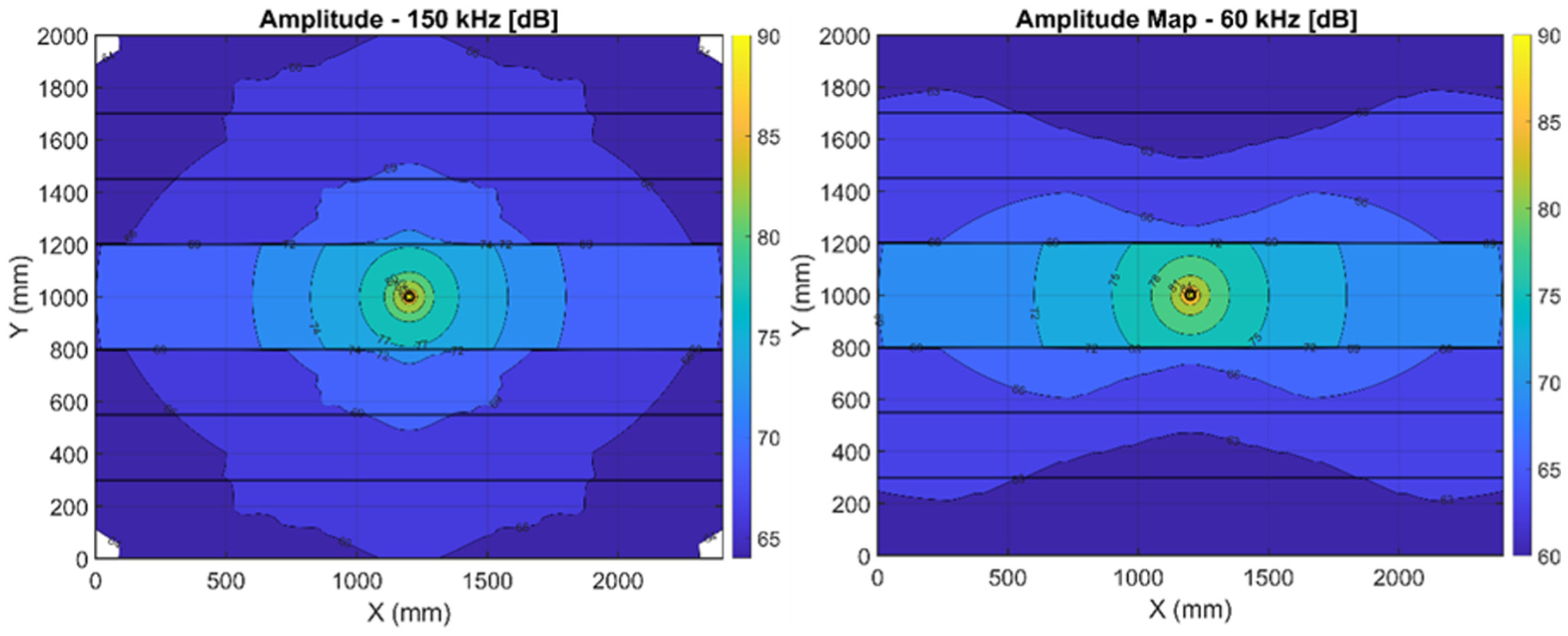
Amplitude maps for 150 kHz (left) and 60 kHz (right) for perfect weld conditions.
Since the difference between transmission under perfect weld conditions (simulation) and realistic welds (experiments) remains within an acceptable range of 5 dB, the use of simulation results to construct these amplitude maps is justified and can offer reliable insights into wave propagation behaviour.
Discussions
The improved estimation of the amplitude by this work can be useful in two contexts. The first context, as demonstrated in this paper, relates to better estimation of the transmission loss of stiffeners. This can lead to an enhanced assessment of the coverage area of AE sensors. The second application is related to characterization of damage using AE, for which parametrized features of the signal are often used. Signal amplitude is one of the most-commonly used features. Although damage characterization is not part of the scope of this paper, the amplitude correction algorithm proposed in this work is expected to improve source amplitude reconstruction thereby enabling improved damage characterization.
It is worth noting that under representative conditions, the operational environment on ships is characterized by higher levels of background noise compared to laboratory settings. The main sources of this noise include machinery, propulsion systems and environmental influences. Measurements conducted by the authors under operational conditions on multiple ships (unpublished) have shown that, within the frequency range analysed in this study, the background noise level is predominantly below 50 dB. This is considered to provide sufficient margin for detecting the expected damage-induced AE signals, even in the presence of a few stiffeners between the AE source and the measurement point in practical applications. In cases where the noise floor exceeds 50 dB, the effective coverage of AE monitoring would be expected to decrease accordingly.
When applying the findings of this study to larger and more complex structural configurations, presence of additional stiffeners can generally introduce additional complexities beyond amplitude reduction, such as multiple reflections and mode conversion. However, in the context of AE monitoring, where signal processing primarily relies on the first-arrival wave packet, such late arrivals (due to longer effective distances and conversion to modes with lower c g ) can be readily windowed out and hence expected to have negligible influence on the analysis. In situations where due to the geometry of stiffeners, sub-optimum sensor layout and/or relative positioning of the AE source the arrival time of additional reflected wave packets turns out to interfere with the first-arrival packet, additional measures will have to be taken in order to split the contributions.
Conclusions
This paper has investigated the influence of stiffeners on the propagation of AE waves in ship structures. Before addressing the transmission coefficient computations, an algorithm to characterize the influence of the sensor transfer functions has been developed. With the use of this algorithm, correction coefficients have been computed, to take into account the influence of the sensors when addressing the wave propagation. These correction coefficients have been computed for different sensors of different frequencies and then have been applied to the measured amplitudes before using them in the transmission computations. This process has been carried out for different wave modes and different frequencies, with the use of both numerical simulations (SEM) and experimental results.
According to what has been found, the variation in transfer functions among sensors of the same type can reach up to 10 dB, introducing discrepancies in recorded amplitudes that are not related to the actual wavefield. Separately, comparison between numerical and experimental investigations indicates that realistically welded stiffeners introduce a transmission loss between 2 and 5 dB relative to perfectly welded joints. As the variability associated with sensor transfer functions is comparable and in some cases exceeds the amplitude attenuation due to welded joints, compensating for the sensor response is critical. Failure to do so would result in amplitude differences dominated by sensor characteristics rather than structural effects.
The results of this study offer a starting point for assessing the limitations of measuring individual AE signals, originating from crack initiation and propagation, due to the presence of background noise and stiffeners. This is part of a wider context for assessing the probability of damage detection based on AE signals. Future work will focus on developing a correlation between the identified influencing factors (sensor response and structural stiffening) and the key SHM objectives of AE-based monitoring, namely damage localization accuracy and damage estimation. This will involve the reconstruction of AE source features from corrected amplitude data and their integration into a framework for damage assessment under realistic ship conditions. Since in the current paper the measurements were restricted to the analysis of A0 waves due to instrumentation limitations, future work should also include comparison between the two fundamental wave modes.
Footnotes
Declaration of conflicting interests
The authors declared no potential conflicts of interest with respect to the research, authorship and/or publication of this article.
Funding
The authors disclosed receipt of the following financial support for the research, authorship and/or publication of this article: This research has been performed in the context of FUSION project. The authors acknowledge The Netherland Organization for Scientific Research (NWO) and project partners for co-funding and technical support.