
Abstract
This article presents an approach to identify naturally developed damage in low-speed bearings using waveform-similarity-based clustering of acoustic emissions (AEs) under fatigue loading. The approach is motivated by the notation that each recorded AE signal from a particular damage is defined by the convolution of the source signal, transfer function of the propagation path and transfer function of the utilised sensor, and may thusly be used to identify consistent AE sources, for example due to crack growth. A sequential clustering procedure is proposed, that is based on waveform cross-correlation. The supporting theoretical background of waveform similarity, rooted in an analytical formulation of waveform propagation and transmission in complex structures, is discussed. The presented methodology is evaluated through application to AE data obtained in a low-speed run-to-failure experiment utilising a densely instrumented purpose-built linear bearing segment. The implemented sensor system comprises arrays of three types of AE transducers, that is relatively low - (40–100 kHz), mid - (95–180 kHz) and high-frequency (180–580 kHz), that are situated on both the raceways and supporting substructures of either side of the bearing. Over the course of 225,000 cycles of extension and retraction, wear has been developed. A total of about ∼2,300,000 AE signals have been recorded. Analysis of the recorded data suggests the rate of degradation increases from around 70,000 cycles onwards. Highly consistent structures of clusters indicative of a localised defect in the raceway have been identified from around 170,000 cycles onwards. These clusters are characterised by hit-rates in the range of 1–2 hits per cycle and an average similarity of 93%, they comprise about half the AE activity for the periods they have been identified for. These results highlight that the proposed cross-correlation-based clustering of AE waveforms and identification of multi-channel formations in said clusters compose a suitable methodology for assessment of damage in low-speed roller bearings.
Keywords
Highlights
An analytical framework for description of acoustic emission (AE) signals and propagation in low-speed roller bearings is presented.
A waveform-similarity-based sequential clustering approach for identification of AE source mechanisms in low-speed roller bearings is proposed.
A run-to-failure experiment utilising a densely instrumented large-scale bearing mock-up has been conducted.
Severe wear comprising of increased surface roughness, grooving and slight pitting has been naturally developed over the course of approximately 225,000 cycles.
Highly consistent structures of waveform clusters indicative of possible localised defect in the raceway have been identified.
The combined clustering and event-building provides a promising methodology for isolating significant AE activity.
Introduction
The integrity of large-scale low-speed roller bearings is essential to the safe and continued operation of the offshore energy infrastructure and its associated activities. Notable applications of these bearings include slew bearings of heavy-lifting cranes, turntables in single-point mooring systems and nacelle-slew or blade-pitch bearings in wind turbines, and as such comprise both installations for the oil and gas and renewables industry, as well as equipment supporting the energy transition. In these offshore applications, bearings are subjected to an unpredictable interaction of operational and motion-induced loading while also suffering from the harsh seawater environment. This combination of high loads and intermittent movement is a generally unfavourable operational condition from the perspective of lubrication, as they may lead to a reduced or broken lubrication film, which has a significant impact on wear. To assure the integrity of these large-scale low-speed roller bearings, robust methodologies for their condition monitoring are required.
Development of wear in rolling element bearings is a complex process of multiple interconnected degradation mechanisms. 1 These may generally be grouped into fatigue cracking, adhesive wear and abrasive wear. 2 Rolling elements that are starved of lubrication, either due to improper maintenance or due to unfavourable operation, operate in a regime of high friction, and are thus particularly susceptible to adhesive wear. The resulting surface degradation induces stress concentrations, which could lead to pitting and micro-cracking. In contrast, sufficient lubrication provides a regime of low friction, which under repeated loading inevitably leads to subsurface crack initiation and the eventual development of spalls. In particular, case-hardened raceways are susceptible to subsurface damage on the interface between the hardened material and the softer substrate. 2 All of these degradation mechanisms eventually produce debris particles, and together with particles that may be introduced through improper maintenance, these act as the asperities that initiate abrasive wear.
Regarding wear, in a critique on common experimental practice, Bhadeshia 2 remarks that increasing contact stresses, as a means to accelerate wear, likely influences the interaction of the interconnected degradation mechanisms, resulting in a different damage evolution process compared to the nominal design life. A similar remark may be extended to the common practice in bearing condition monitoring research of introducing artificial damage, as such simulated damage does not cover the interconnected nature of wear in rolling element bearings.
To monitor degradation in rolling element bearings, several techniques have been suggested to date. Most conventional are the applications of strain and vibration monitoring,3,4 which may be effective in high-speed applications, but suffer from decreased detectability at low speeds. On alternatives, comprehensive review studies have been published,5–8 which include techniques such as lubrication analysis, 9 electrostatic monitoring 10 and temperature monitoring. 11 In this study, passively generated acoustic emissions (AEs) are explored, for their potential to detect early-stage degradation. AE refers to the release of energy as elastic stress waves in a material when the microstructure of said material is irreversibly altered (e.g. crack growth or dislocation movement). The analysis of AE signals in a bearing is a non-trivial challenge, due to the complex geometry and interfaces giving rise to additional reflection, scattering and diffraction of the ultrasonic waves.
The prior art on the application of AE techniques for bearing condition monitoring seems to originate with Balderston, 12 who identified it as promising in 1969. In the subsequent decades, a few other investigations have been reported, describing experimental studies of AE bearing condition monitoring. Of primary interest is the combination of naturally introduced damage and very-low speed (<20 rpm), for which literature is limited due to the practical challenges associated with developing the degradation. In some early studies, this problem is mitigated by performing in-situ tests,13,14 or by evaluating naturally pre-worn bearings from industry applications in the laboratory. 15 A downside of these approaches is the loss of information on the progression on the damage; however, these studies have successfully demonstrated a greater sensitivity of AE compared to vibration monitoring at low speeds. Also particularly Mba et al. 14 observed that the recorded waveforms are specific to the propagation path between source and receiver. Moreover, if the bearing may be considered nearly static relative to the propagating elastic stress waves, transmission of those stress waves in between the rolling elements is expected to remain measurable by proper hardware and sensor layout despite substantial losses.16,17 Sako and Yoshie 18 identified naturally developed flaking in a small-scale bearing at speeds between 1 and 10 rpm. However, the induced damage was the result of running for 98% of the lifetime at 400 rpm while overloading the bearing in the range of plastic deformation. Liu et al. 19 applied cyclostationary frequencies to evaluate a naturally worn bearing from a 15-year-old wind turbine at speeds ranging 0.5–5 rpm, while using discrete/random separation-based cepstrum editing liftering to amplify weak fault features from the AE signal. Finally, Caesarendra et al. 20 studied the development of degradation in a run-to-failure experiment lasting nearly 300 days, and identified a significant change in the bearing condition through conventional AE features.
Regarding studies on naturally induced damage at higher speeds (>60 rpm), Li et al. 21 successfully differentiated between minor and major wear through evaluation of waveform features. Elforjani and Mba observed a correlation between increasing AE energy and the evolution of cracks and spalls in bearings22–27 and made an attempt to estimate the size of surface defects from the AE signal duration. 28 Elforjani 29 also applied artificial neural networks to predict the remaining useful life of a grease-starved bearing. With further increasing speed, studies on applications of cyclostationary techniques become of note,30–33 which also propose down-sampling of continuous AE data to ease data handling. 34 The correlation between AE energy and damage evolution and severity is further explored.35,36 Hidle et al. 37 propose a detector for subsurface cracks based on the pulse integration method. And in comparative studies also involving vibration monitoring, AE demonstrates earlier damage detection36,38 – particularly when combined with spectral kurtosis 33 – and fusion of vibration and AE data has shown to increase the reliability with respect to either method separately. 39 Besides these, k-means clustering of AE waveform features has been applied to identify crack initiation and propagation. 40 A correlation has been observed between lubrication film thickness and AE energy.41,42 Furthermore, in a fundamental study on rolling contacts, a correlation has been reported between evolving surface damage and the AE hit-rate. 43
Although experiments involving artificially introduced damage are not considered representative of those involving naturally developed degradation, these studies may still provide informative insights regarding the effectiveness of the explored signal processing techniques. Broad speed-range (10–1800 rpm) assessments have been performed by Smith 4 and McFadden and Smith. 44 For very-low speeds (∼1 rpm), later studies implemented classification through autoregressive coefficients to differentiate between the unique transmission paths of several artificially introduced damages, 45 and ensemble empirical mode decomposition with multiscale principle component analysis 46 or multiscale wavelet decomposition 47 to identify the damaged component through characteristic frequencies. The applicability of multiscale wavelet decomposition was also demonstrated at a somewhat higher speed representative of the main bearing of a wind turbine. 48 For a similar speed range (20–80 rpm), in comparisons between relevance vector machine (RVM) and support vector machine, RVM was demonstrated to be effective at classifying several damages in different components.49,50 In high-noise environments, both artificial surface and sub-surface defects were identified by applying probabilistic techniques (Gaussian mixture model) to differentiate between damage-initiated energy and background noise. 51
With further increasing speed, again cyclostationary techniques are explored for localised defects,52–54 with studies reporting improved early detection through the application of short-time techniques,55,56 spectral correlation 57 and spectral kurtosis, 58 and studies reporting improved performance in a high-noise environment by applying self-adaptive noise cancellation, 59 least mean squares filtering60–62 or wavelet-based filtering.63–65 Additionally, machine learning techniques, such as neural networks, have been suggested and implemented to identify characteristic defect frequencies from spectrograms.66,67 Alternative to cyclostationary techniques, time-of-arrival-based localisation is demonstrated for the detection of localised defects in static raceways, 68 and the fusion of AE and vibration-based multi-feature entropy distance is proposed for damaged-component identification. 69 In the same context, the sensitivity of several AE features to various operational conditions has been evaluated.70–75 Also a correlation between defect size and the AE burst duration and amplitude is reported.76–79 Synonymous to the burst duration, this correlation has been observed for ringdown counts, 80 and the time difference between double bursts as well.64,81 Material protrusions above the mean surface roughness were identified as the AE source mechanism of artificially introduced defects. 82
Regarding lubrication contamination, literature typically describes experiments involving highly controlled contaminated lubrication samples, which should be classified as artificial damage. However, the processes that generate the stress waves from the presence of the contaminated particles may remain comparable to the one for naturally contaminated lubrication, provided that the contaminated samples are sufficiently representative of actual contamination. Studies have shown that the size, weight and hardness of the particles are correlated to the amplitude of AE signals.77,83–86 Also, the number of particles seems to correlate to the hit-rate of the contamination initiated signals.77,83 Besides these conventional characterisation approaches, machine learning algorithms – such as sparse dictionary learning 87 and a convolutional neural network 88 – have also been applied in early-stage studies to differentiate between contaminated and uncontaminated lubrication.
In this article, detection and identification of degradation-induced ultrasonic signals in low-speed roller bearings have been experimentally investigated. A similarity-clustering-based approach for the identification of consistent emission sources is implemented for detection of AE from consistent degradation modes (e.g. crack growth). It is applied to an experimental evaluation of naturally developing degradation in a large-scale highly loaded low-speed roller bearing. The section ‘Methodology’ discusses the framework and identification approach, while the section ‘Experimental setup’ describes the test setup, instrumentation and experimental procedures. In the section ‘Results and discussion’, the results of a natural degradation experiment are presented, and the framework and identification approach are evaluated and discussed. Finally the section ‘Conclusions’ provides the conclusions of this study.
Methodology
Identification of developing degradation in rolling elements may follow directly from the identification of AE source signals. In an idealised situation, instrumentation is situated close to the source of emission, that is where damage is evolving. There, the recorded signal is nearest in form to the original source signal, and therefore, the task of identifying the mechanism of emission is most apparent. In practice, instrumentation on the raceway can typically not be realised, and therefore generalisation to the external surface of a bearing – or the substructure – is necessary. This generalisation is demonstrated analytically in this article. Experimentally, the concept is applied to identify naturally evolving damage in a bearing. A purpose-built linear bearing is used in the experiment, as depicted in Figure 1, which is designed to provide the ability to instrument both the raceways and substructure, to assess the identification procedure for both instrumentation scenarios.
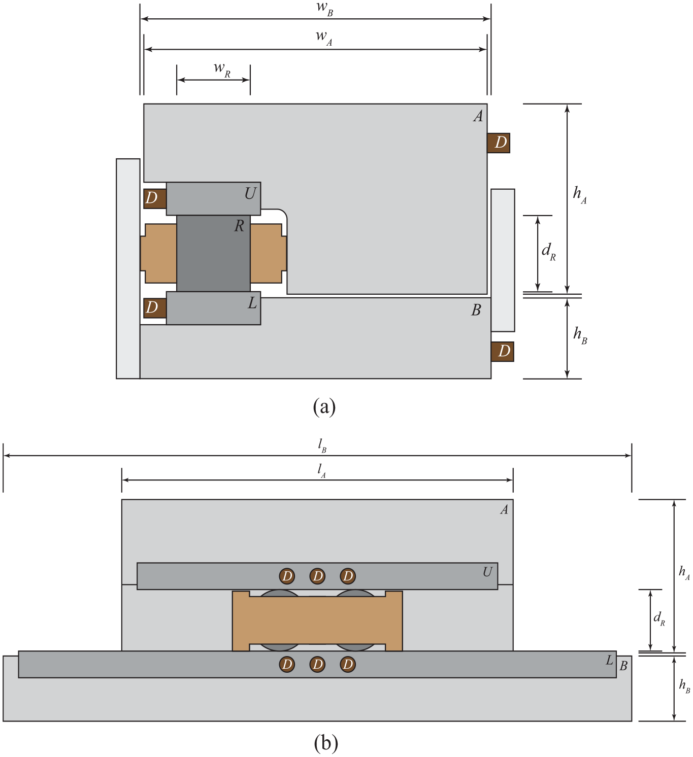
Illustrations of test setup (to scale, top section), showing (a) a cross-section of the bearing with component identifiers and (b) a front view of the bearing without the cover plate. Indicated components are the roller (R), the nose raceway (L), the support raceway (U), the nose substructure (B), the support substructure (A) and the sensor arrays (D). Dimensions used in this research are given in Table 1.
For the rolling elements of a bearing, three principal regions may be identified for degradation-induced sources. Figure 2 illustrates these, which are (a) subsurface in the raceway, (b) subsurface in the roller, and (c) the interface of roller and raceway. Evading the challenges of instrumenting a roller, the closest instrumentation could at best be situated directly on the raceway. However, in practice instrumentation on the raceway is often not feasible, and therefore sensors are often situated on the support structure – further away from the source. The effect of this extra distance on the transformation on the source signal is discussed in detail for the three identified cases. The notation is motivated by the system proposed by Berkhout 89 that was also utilised by Pahlavan et al.90,91 and Scheeren et al. 13
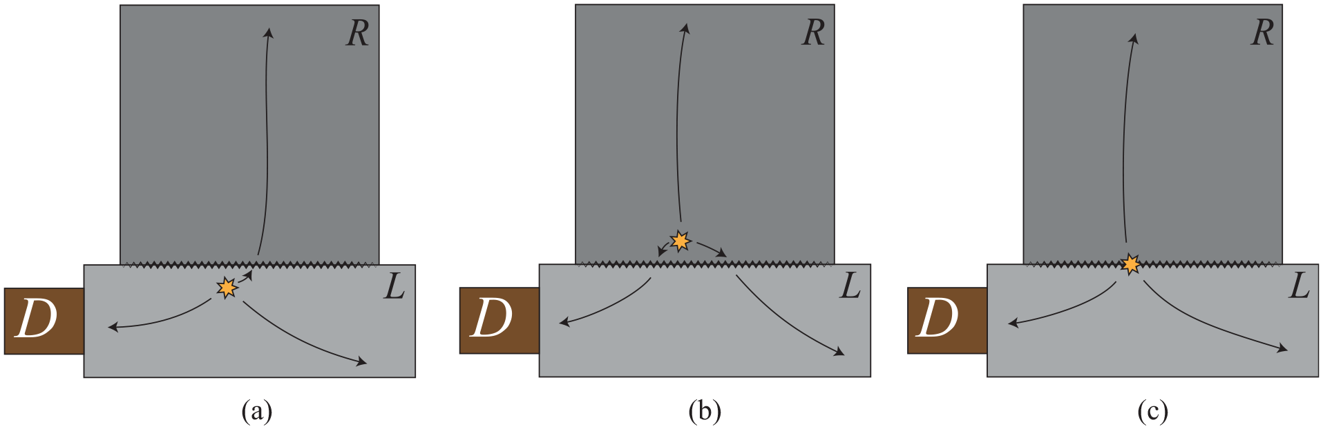
Three alternative source configurations with primary transfer paths, showing (a) a subsurface source in the raceway, (b) a subsurface source in the roller and (c) a source on the interface between roller and raceway.
Considering a subsurface crack that is propagating in the nose raceway, as illustrated by Figure 2(a), a recording from a receiver on that same raceway may be described in the frequency domain as

Herein,
That same source signal will also be transmitted over the interfaces, through the roller, into the opposing raceway. If in transmission it retains sufficient energy to surpass the ultrasonic background noise, and to be detectable by a receiver on that opposing raceway, the recorded signal may be described by
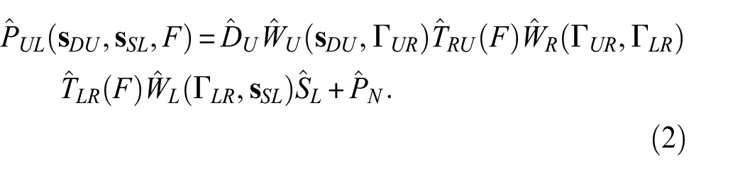
Herein,
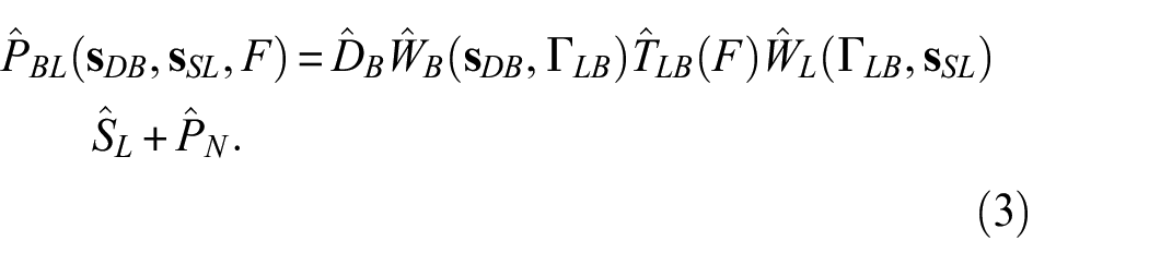
The propagation and transmission captured in Equations (1) and (2) describe cases where instrumentation may be realised close to the expected source location. If this is not the case, sensors might be situated further away, and as in this case, possibly on a substructure. Herein, a recorded signal on the substructure of the nose ring essentially represents an extension of Equation (1), and may be characterised by
Herein,
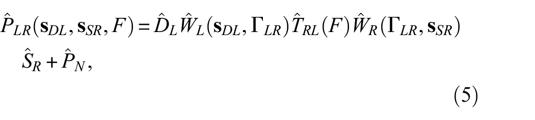
Similarly, a recording on the substructure of the support ring essentially represents an extension of Equation (2), and this signal may be characterised by
Herein,
When comparing the signals on both raceways, it may be noted the relative difference between these signals is primarily the result of transmission through the roller, as long as the propagation functions for the raceways may be considered similar (
Under these assumptions, it is expected that the relative difference in the energy retained by the signal when comparing Equations (1) and (2) is in the same order as the loss for Equations (3) and (4), and for both this difference is primarily characterised by the transmission through the roller. This specific pattern may be used to identify the raceway as the origin of a source signal.
Alternatively, a sub-surface crack may be propagating in the roller, as depicted in Figure 2(b). For this source mechanism, the detected signals at the same four sensor locations may be described as
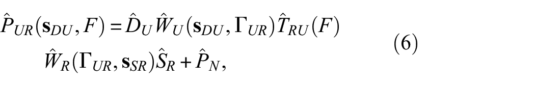
and
Herein,
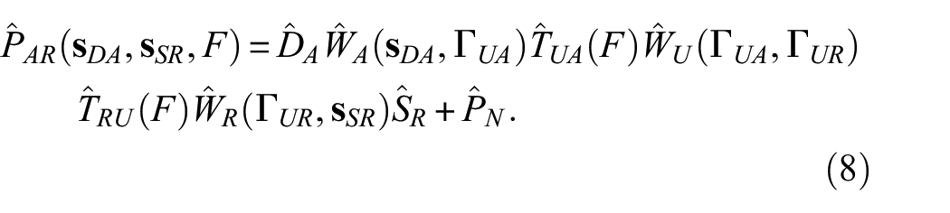
Apparent for this source is the shift towards a more symmetrical set of equations, in comparison to those for the source in the raceway. Regarding the transformations that make up the primary transmission path, Equations (5) and (6), and Equations (7) and (8) show semblance. The geometry contains a similar symmetry in dimensioning, as depicted to scale in Figure 1. This symmetry in primary transmission paths is expected to provide a basis for identifying degradation in rollers.
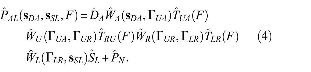
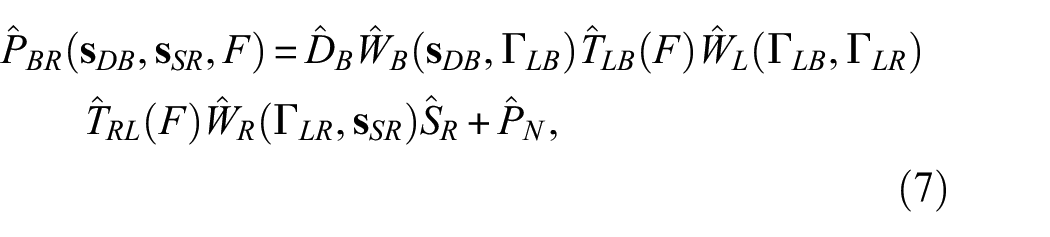
Lastly, for a source on the interface between the roller and raceway, as illustrated in Figure 2(c), that may be due to contamination of the lubricant, the recorded signals may be described as

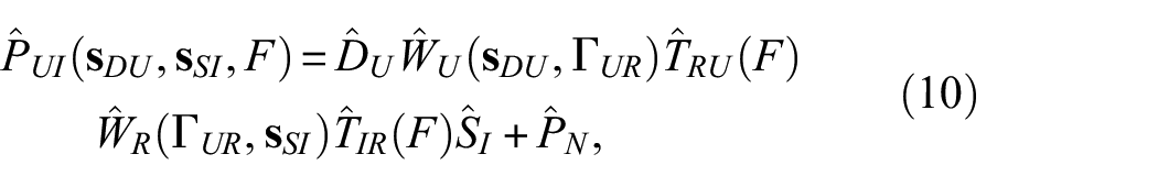
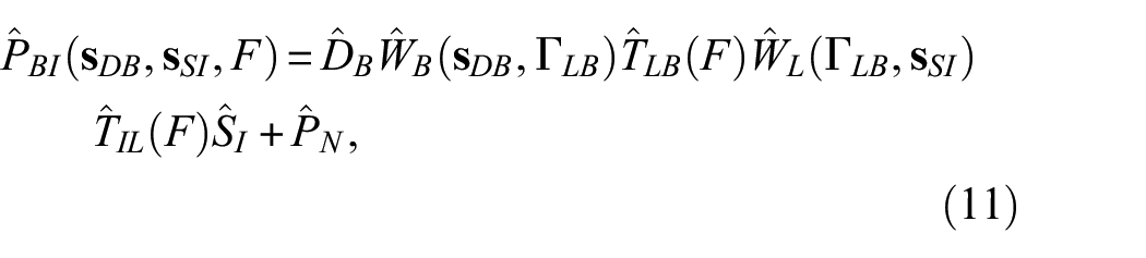
and
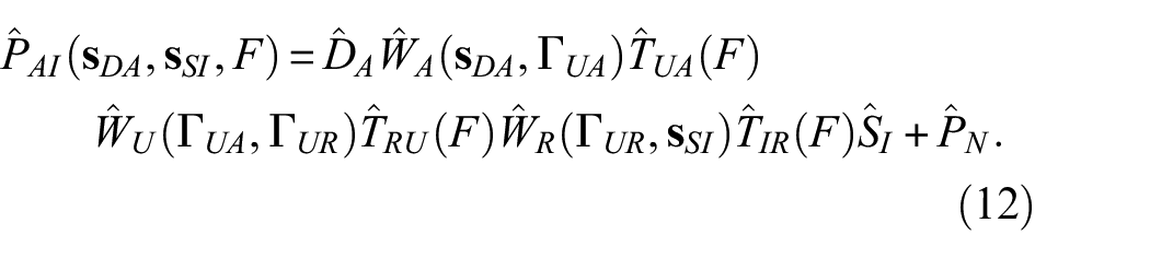
Herein,
The resulting set of equations is characterised as being in between the sets with the source signal in the roller or raceway, with the difference being how it incorporates transmission through the roller.
These three systems of equation show that from a combination of recordings from two sensors, of which one on the nose ring and one on the support ring, the component where the source signal originates from may be identified.
Clustering
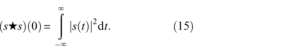
To identify mechanisms that consistently emit elastic stress waves, such as crack growth, consistency in the source signals must be sought for. Implementation of this procedure is based on clustering signals by cross-correlation, which is defined in the time domain as

wherein
The similarity index may be obtained by taking the normalised absolute maximum of the cross-correlation, that is
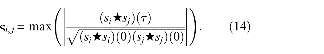
Herein,
The result of Equation (14) is a similarity value that is contained within the closed interval
In line with Equations (1)–(12), the procedure for cross-correlation may also be expressed in the frequency domain as
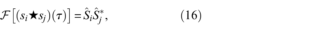
with
This cross-correlation is determined based on the emitted source signals, whereas in monitoring, the recorded response at locations other than the source is obtained. The source signal is the deconvolution from the recorded response, and may be represented as

wherein
Using this, the cross-correlation of source signals may also be expressed as
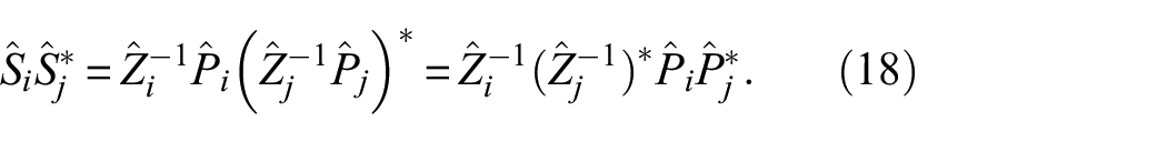
Here the distributive property in convolution of the complex conjugate and the associative and commutative properties of the convolution allow for reorganisation of the cross-correlation into the convolution of the individual cross-correlations of the inverse transfer paths and the recorded responses.
Also considering associativity with scalar multiplication, and Plancherel’s theorem on the equivalence of the integral of a function’s squared modulus in the time domain and frequency domain, the normalisation may be expressed by
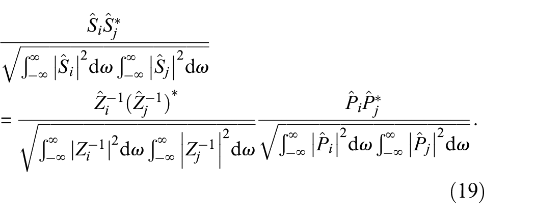
The similarity is defined as the absolute maximum of the normalised cross-correlation in the time domain. Therefore, the inverse Fourier transform is used to return to the time domain. Herein, the convolution theorem allows for the separation of the
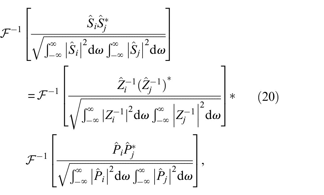
with * denoting the convolution operator.
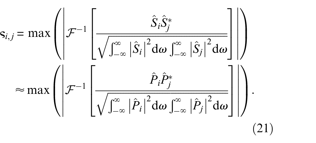
Under the assumption of near-identical transfer paths (
From the similarity between signals, the dissimilarity may be defined as

This dissimilarity
To identify structure in signal (dis)similarity, a particularly suitable approach is agglomerative hierarchical clustering (AHC), of which implementations by Van Steen et al. 92 and Huijer et al. 93 are illustrative. This bottom-up approach links signals by increasing dissimilarity, to generate a dendrogram that shows the connectivity of all elements of the dataset. From the dendrogram, clusters may be obtained – amongst other procedures – by cutting the branches at a certain dissimilarity threshold.
A downside of AHC – and many other clustering approaches – is the requirement to have all of the data known at the beginning of the procedure, hindering online implementation. Also the requirement to know the distances between all data points makes it less suitable for large datasets. Alternative sequential, or incremental, algorithms have been proposed, for which the general procedure is to compare each new signal to the already formed clusters, and to assign said signal to either one of those clusters or assign it as a new cluster.94–97
A basic sequential clustering algorithm is implemented that is particularly aimed at clustering highly similar signals. The following procedure is adopted: In order of detection, each signal is first compared to all already identified clusters – in case there are none yet, this step is omitted. If the dissimilarity between the evaluated waveform and any existing cluster is lower than a predetermined threshold, the waveforms gets associated with the cluster of lowest dissimilarity. If no cluster of sufficiently low dissimilarity is identified, a second comparison to the sample of other non-clustered waveforms takes place. If in this second comparison a sufficiently low dissimilarity is observed, the waveforms with the lowest similarity will together form a new cluster. If in no comparison the dissimilarity threshold is met, the evaluated waveform gets assigned to the sample of non-clustered waveforms. This procedure is graphically illustrated in Figure 3.
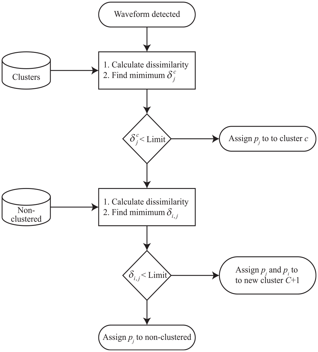
Overview of clustering procedure.
To reduce the computational burden, only a limited sample of waveforms is compared for each cluster and for the non-clustered waveforms. In case of the latter, a moving window is utilised that only considers the last 250 signals that were assigned non-clustered. The reasoning being that more recent signals are more likely to meaningfully correlate to each other. The same reasoning has also been used to implement a procedure that declares clusters as dormant after 250 consecutive unsuccessful comparisons, to eliminate needless comparisons to a significant portion of insignificant clusters composed of only a few hits. Clusters larger than 50 hits are excluded from the dormancy check. For each cluster, a sample of up to nine waveforms is selected. To suitably represent the cluster as a whole, the sample contains some of the very first, some of the very last and some arbitrary signals from the cluster. Due to the use of a low dissimilarity threshold, the high similarity within the cluster assures any selection from the cluster represents the cluster as a whole.
For the comparison of waveforms to clusters, a weighted average dissimilarity measure is used. Weighing is applied to increase the importance of newer additions to the cluster, and decrease the importance of the original waveforms. This improves the resilience of the clustering approach to slight and gradual changes in the clustered signals, which may occur due to the influence that the degrading geometry might have on the transmission of the source signal. To determine the weighted average, the approach uses
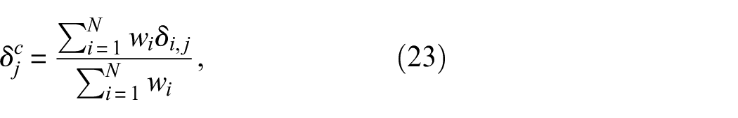
wherein
Experimental setup
A test setup that is representative of a segment of a large-scale slew or turret bearing has been utilised. It consists of a double linear bearing, which, under vertical load applied through the support rings, allows for cyclic horizontal movement of the nose ring. The illustrations in Figure 1 show the top half of the designed setup. The bottom half is an exact vertically mirrored copy of the top half, with both halves separated by a fibre-reinforced composite panel for improved ultrasonic isolation. A picture of the setup with a three-roller configuration prior to the application of grease is shown in Figure 4. Note that the same setup has also been used in Scheeren and Pahlavan 14 for different experiments on low-speed roller bearings.
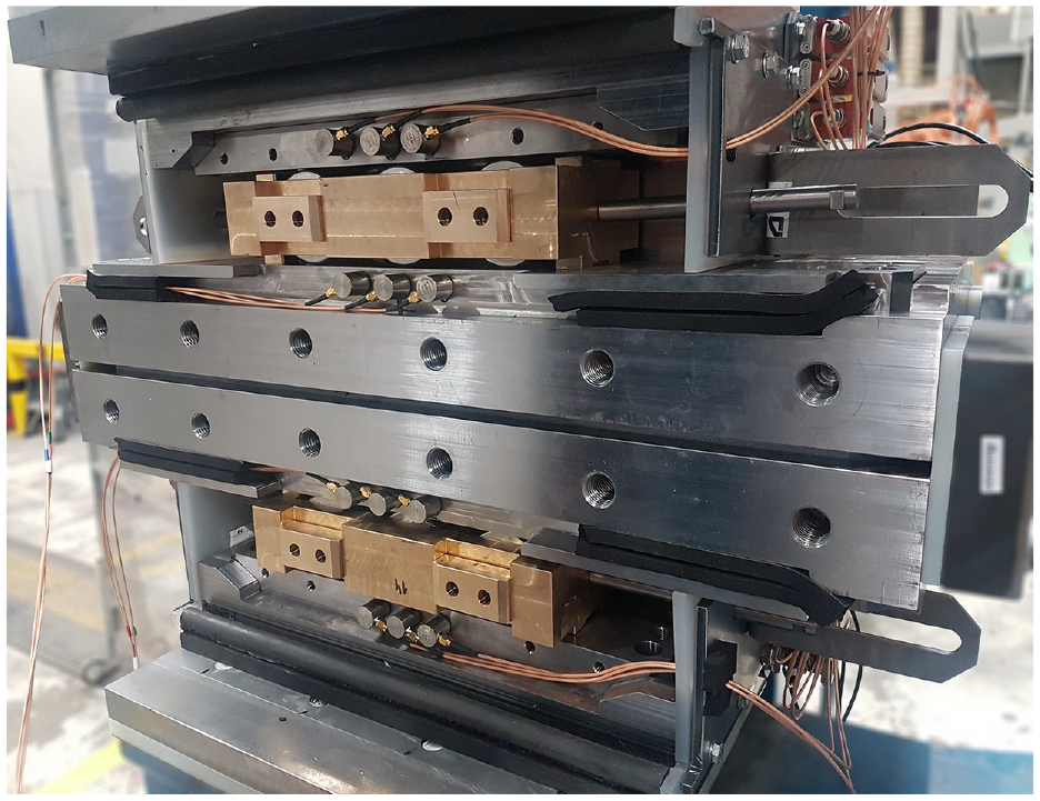
Picture of experimental setup with cover plates removed.
The raceways, rollers and cages are all modular components. The experiment described in this article uses in each half of the setup two raceways with a thickness of 32.5 mm made out of Hardox 600, two rollers with diameter of 69 mm made out of 100Cr6 through hardened bearing steel and a cage made out of CuSn12C tin bronze. Out of the notable permanent components, the nose and support substructures are all made out of S355J2 structural steel. The main dimensions of the setup, as indicated in Figure 1, are given in Table 1.
Main dimensions of test setup.
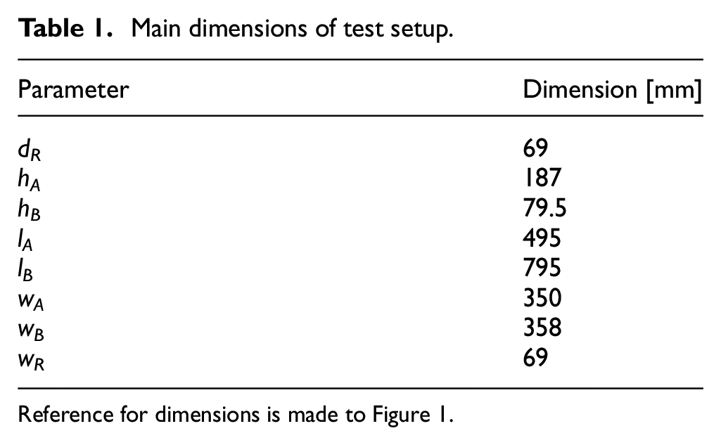
Reference for dimensions is made to Figure 1.
Instrumentation
Ultrasonic signals generated over the course of the natural degradation test have been recorded in the frequency range of 40–580 kHz. To achieve this, the setup has been instrumented on eight locations with three types of commercial piezoelectric AE transducers. An overview of the locations and sensor types of all measurement channels is given in Table 2.
Overview of measurement channels.
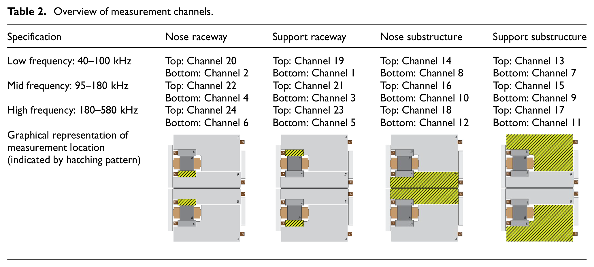
The eight measurement locations are split between the two mirrored test chambers. The isolation in the middle of the nose ring allows for these to be considered acoustically independent from one another. Within the sphere of influence of each chamber, the measurement locations can be identified by a combination of two binary groups. Each array is situated either on the raceway or on the substructure, and that component is part of either the nose ring or the support ring. The illustrations in Figure 1 are representative of the measurement locations for the top chamber, while for the bottom chamber the locations are vertically mirrored.
The eight measurement locations all represent arrays of three sensors – each of which sensitive to a specific part of the considered frequency range. Low frequencies are covered by a 60 kHz resonant R6α, mid frequencies by a 150 kHz resonant R15α and high frequencies by a broadband WSα– all manufactured by Physical Acoustics Corporation (Princeton, NJ, USA). All of the sensors are amplified by external AEP5H pre-amplifiers set to a gain of 40 dB, before being connected to a 24-channel AMSY-6 AE measurement system fitted with ASIP-2/A signal processing cards – both manufactured by Vallen Systeme (Wolfratshausen, Germany). Digital band-pass filters are applied for each sensor type individually to separate low-, mid- and high-frequency content. For the low-frequency measurement channels, a band-pass filter from 40 to 100 kHz is set, for the mid-frequency 95–180 kHz and for the high-frequency 180–580 kHz.
Whenever a 50 dB threshold was crossed, a transient recording of 812 µs sampled at 5 MHz and the extracted feature data are stored. The transient data contains a 200 µs pre-trigger recording to capture the onset of the detected signal prior to crossing the threshold.
Experimental procedure
An arrangement of two rollers is subjected to a vertical load of 1215 kN, while a horizontal stroke of 70 mm is cycled through every 12 s for a linear speed of about 0.012 m/s. The test is expected to continue for 230,000 cycles (approximately 770 h). During the test, the setup is lubricated daily with Interflon LS1/2 heavy duty grease. To compensate for slipping, the rollers and cages in the setup are repositioned whenever they have travelled more than 45 mm from the centred position.
Over the course of the test six inspections are performed at (i) ∼51,000 cycles, (ii) ∼138,000 cycles, (iii) ∼166,000 cycles, (iv) ∼196,000 cycles, (v) ∼211,000 cycles and (vi) ∼225,000 cycles (end of test). Inspections primarily constituted visual observation, additionally wear depth (for roller and raceway) and roundness (for roller) were measured.
Filtering
In pre-processing, two additional procedures for filtering are implemented. These are a signal-to-noise ratio (SNR) filter and a position filter.
Noisy signals are less likely to be clustered when a low dissimilarity threshold is set. Therefore, to remove these noisy signals, an SNR-based filter is implemented. This filter compares the peak amplitude in a 100 µs window before detection to the peak amplitude of the signal. A minimum SNR of 10 (20 dB) is imposed.
To mitigate for signals generated by collisions related to the small gaps between components while cycling, and in particular when reversing the direction, a position-based filter is implemented. This filter separates all signals that occur within 2.5% of the start or the end of the horizontal stroke.
Results and discussion
A total of approximately 225,000 cycles were performed under a load of 1215 kN. After the test, severe wear of the raceways in both the top and bottom chamber was observed. This wear is primarily present in the form of increased surface roughness and grooving, while additionally some slight pitting is observed. Both top and bottom chambers (Figure 4 for reference) generally show a similar severity of wear; however, in each chamber, the lower raceway was worn significantly more than the upper raceway. The rollers generally show wear that is comparable in severity to the upper raceways. Five additional inspections have been performed over the course of the experiment, these observations will be discussed in parallel to the hit-rate observed over the course of the experiment.
An extensive number of ultrasonic signals have been recorded during the experiment. Some damages were also incurred by the sensor system. These damages were primarily sustained in the bottom chamber, where the mid-frequency and broadband sensor were broken off the raceway.
In extension and retraction, the valve system of the horizontal cylinder emits a continuous low-frequency noise, that could be detected by the low-frequency receiver on the support substructure of the bottom half of the setup. The recorded signals for this receiver show a continuous consistent alternation between 6 s of increased noise, and a short period of reduced noise. These patterns have been used to identify the movement of the nose ring, and subsequently filter for 2.5% of the nominal stroke in time. About 98.5% of the cycles could be detected using this procedure. In further processing, the valve-initiated signals are rejected by the SNR filter.
Limiting the analysis to the top chamber, a total of approximately 2,300,000 AE signals have been detected that pass through the SNR and start-stop filters. The ultrasonic activity, represented in form of hit-rate per cycle (i.e. extension and retraction of the horizontal cylinder), is shown in Figure 5, of which the middle two graphs display the channels on the raceways, and the outer graphs display the channels on the substructure. Note that channel 14 detected no signals (that are not removed by the filters) over the course of the experiment. An arbitrary selection of three waveforms from each of the measurement channels on the top chamber of the setup is depicted in Figure 6.
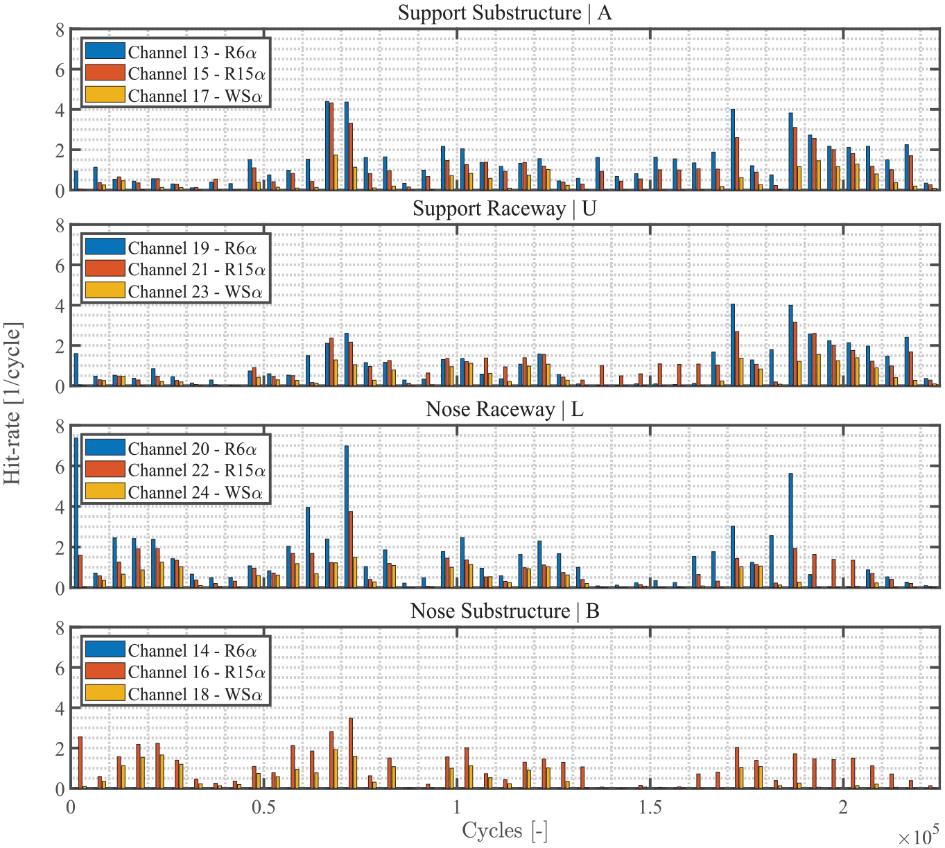
Ultrasonic activity in the top chamber separated in graphs per location: support substructure (top), support raceway (upper middle), nose raceway (lower middle) and nose substructure (bottom).
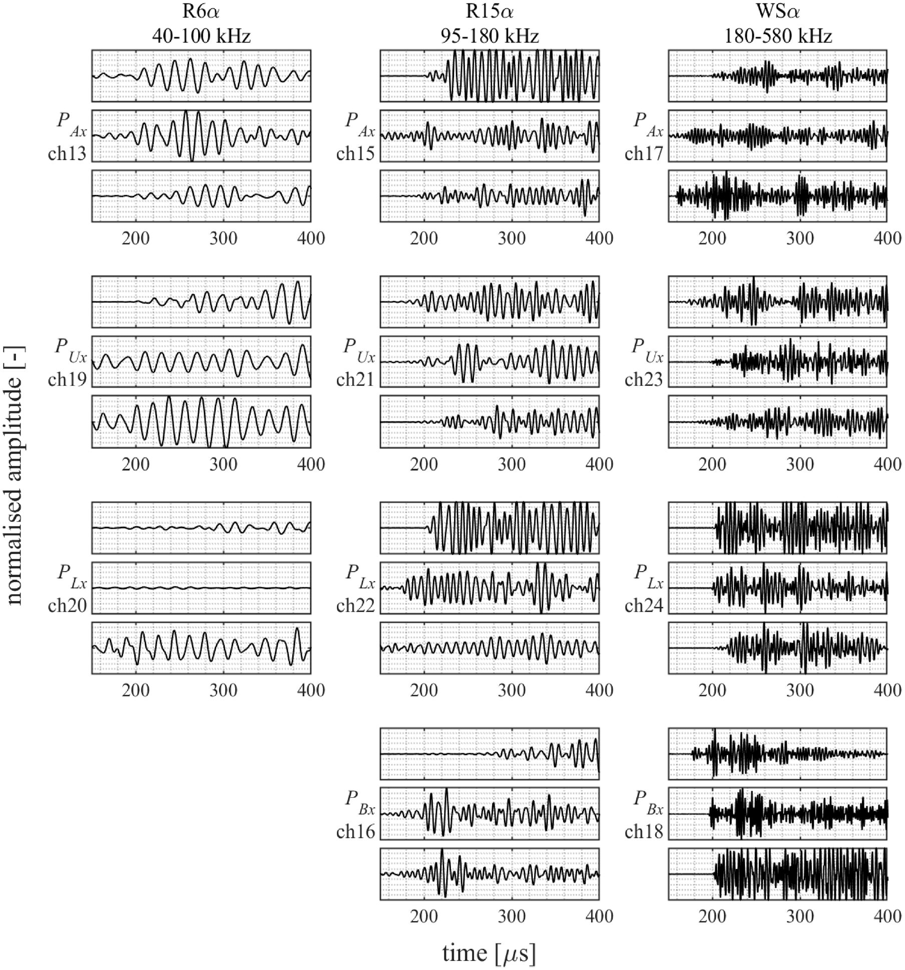
Overview of an arbitrary selection of waveforms recorded on the top chamber.
Considering Figure 5, it seems that from around 70,000 cycles the activity on the raceways increases, possibly related to some form of more significant degradation. A comparable trend can also be observed in the substructure channels. Later on, another significant rise in activity is observed at around 170,000 cycles.
These crude observations in the hit-rates are complemented by intrusive inspections. At 51,000 cycles, the first inspection suggested no significant damage and only slight contamination of the grease was present. For the second inspection at 138,000 cycles – after the first significant increase in hit-rate – wear particles were observed throughout the setup, and the raceways showed excessive wear at the contact area. These observations together with the detected ultrasonic activity suggest that the onset of this wear took place at around 70,000 cycles.
During the third inspection at 165,800 cycles, an increase in the surface roughness of the raceways was observed. Shortly after this observation, AE activity peaked with hit-rates reaching up to 5 detected signals per cycle. Just before the next inspection at 196,300 cycles, activity peaked yet again, with hit-rates again reaching up to 5 hits per cycle. During this inspection, light pitting was observed on the rollers, and the roughness had increased further for both rollers and raceways. For the fifth inspection, around 211,000 cycles, further development of the wear was reported. And the final inspection, at the end of the 225,000 cycles, reported no significant changes compared to the fifth inspection. Several pictures of the resulting degradation of the nose raceway at the end of the experiment are included in Figure 7.
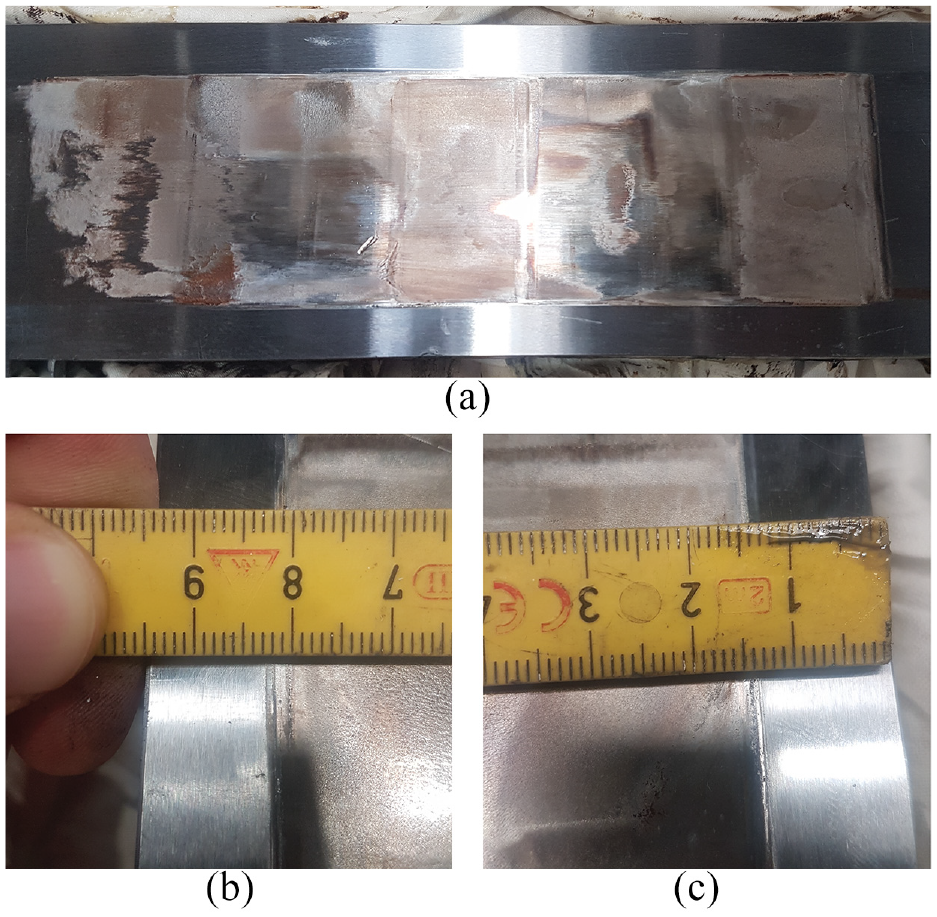
Pictures of post-experiment inspection of nose raceway, showing (a) overall wear pattern comprising increased surface roughness (discoloration), pitting and grooving, (b) close-up of grooving and surface deterioration at the lower edge in (a) and (c) close-up of grooving and surface deterioration at the upper edge in (a).
Overall, it can be concluded that the biggest changes in the observed damage during the inspections match the significance of ultrasonic activity that has been detected. Notable though is that the reported contamination does not seem to cause excessive AE activity.
To identify possible patterns in the ultrasonic activity, the clustering procedures described in the section ‘Methodology’ have been implemented in in-house code developed for MATLAB R2022a. For each of the measurement channels, the 100 largest clusters have been evaluated, and based on common trends among different channels, two structures of significant clusters have been identified. These structures of clusters are shown in Figures 8 and 10, and seem to be related to the significant increase in activity that is observed in Figure 5 at around 170,000 cycles and 190,000 cycles.
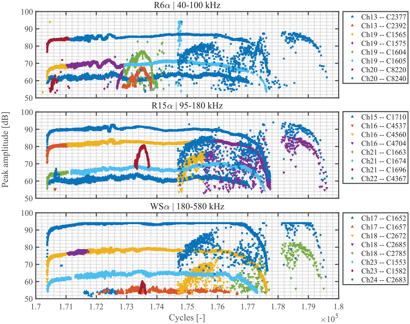
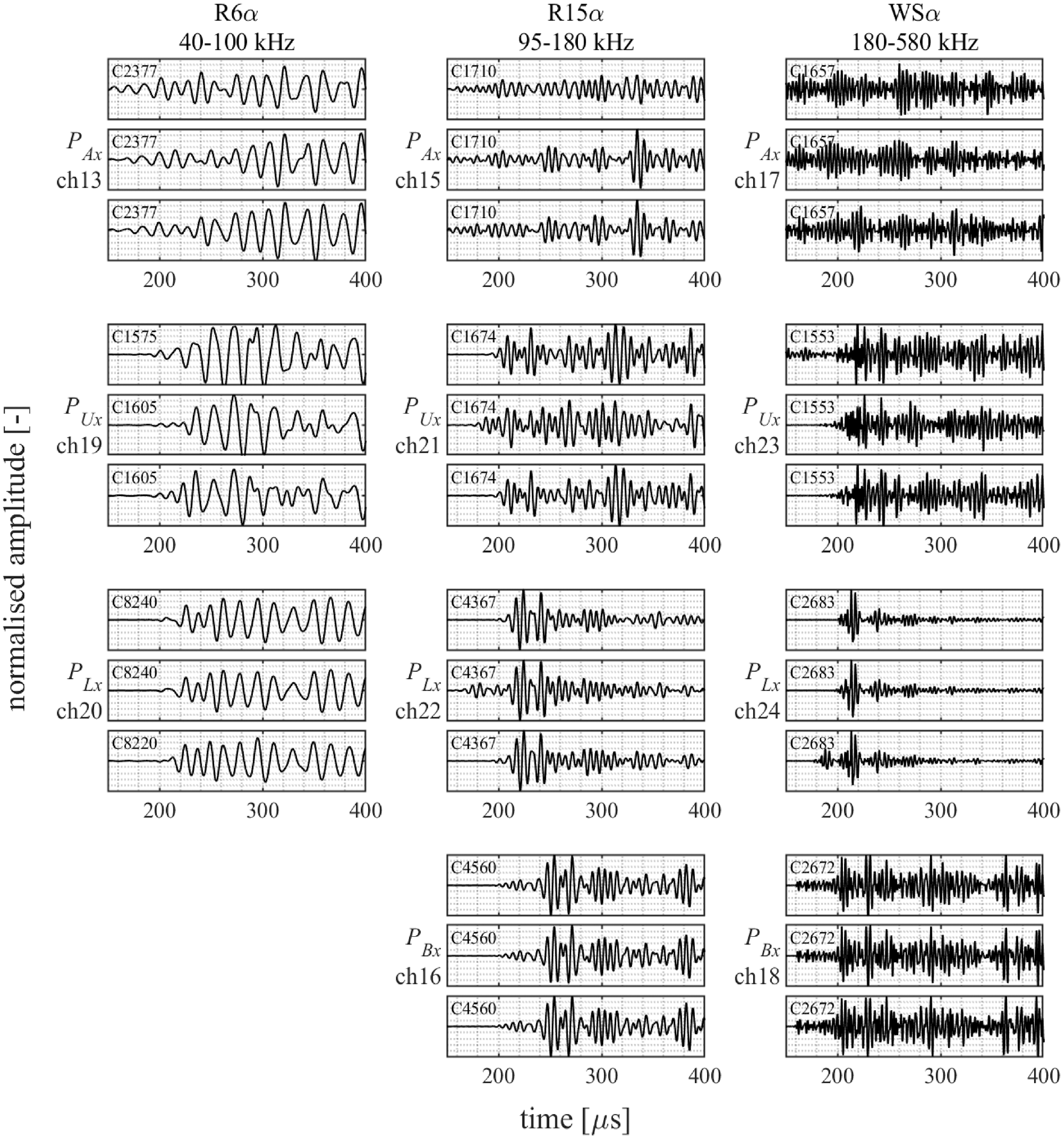
Primary structure of selected clusters from low- (top), mid- (middle) and high-frequency (bottom) measurement channels.
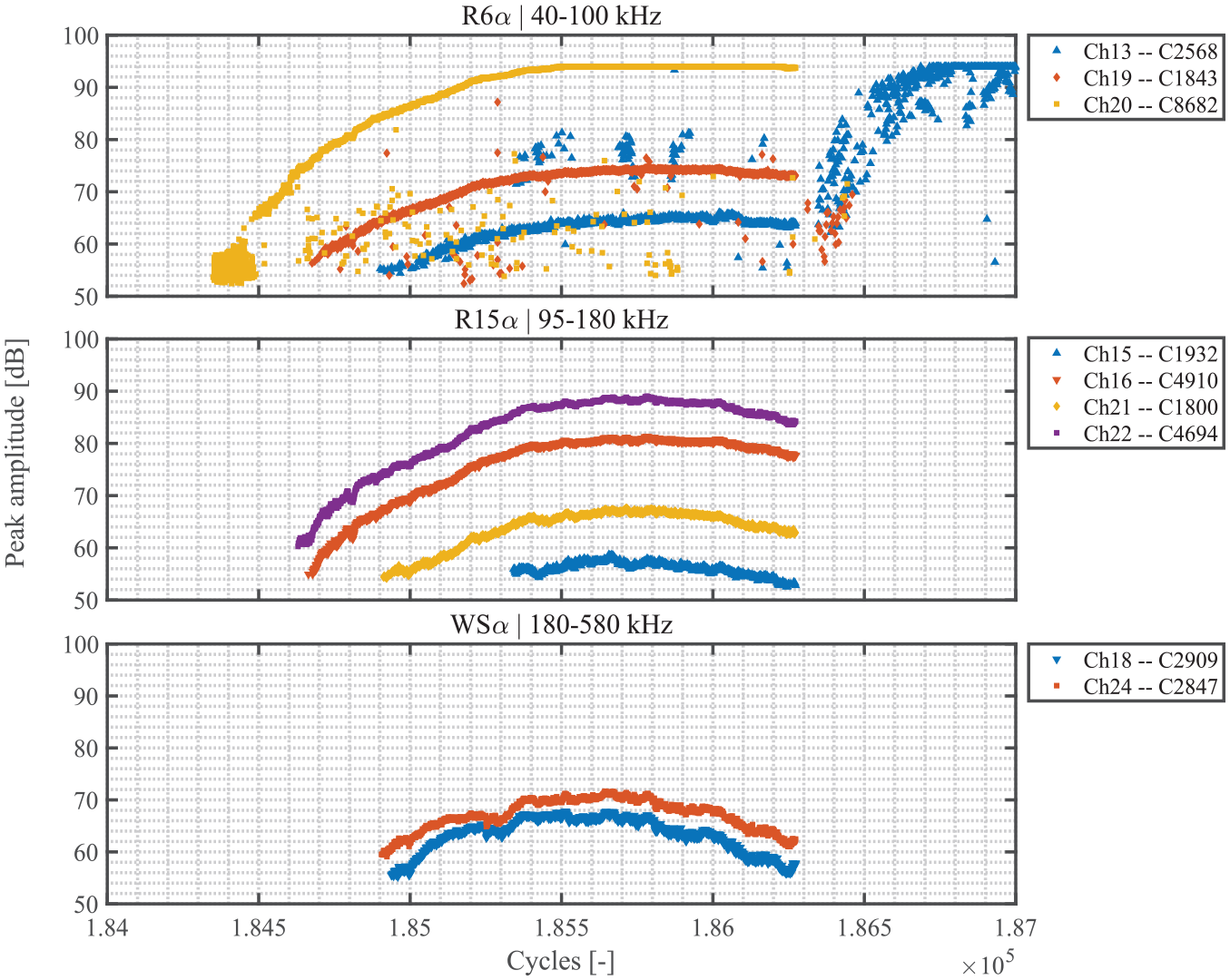
The largest structure of clusters is the one that was encountered between 170,000 cycles and 180,000 cycles, as shown in Figure 8. An arbitrary selection of three illustrative waveforms from each of the measurement channels comprising this structure of clusters is depicted in Figure 9. The structure is composed of about 77,000 AE hits that are detected by 11 of the 12 sensors present on that half of the setup. The average similarity of each waveform to its respective cluster is 0.93, highlighting the concept of consistent signal generation and propagation. The most noticeable averaged activity reaches up to 2 hits per cycle in the mid-frequency range. Comparing this to the hit-rates shown in Figure 5 suggests that the clusters in the structure make up about half of the activity for the hit-rate peak between 170,000 cycles and 180,000 cycles. The rest of the activity is likely to be attributed to less consistent degradation mechanisms, such as wear and contamination.
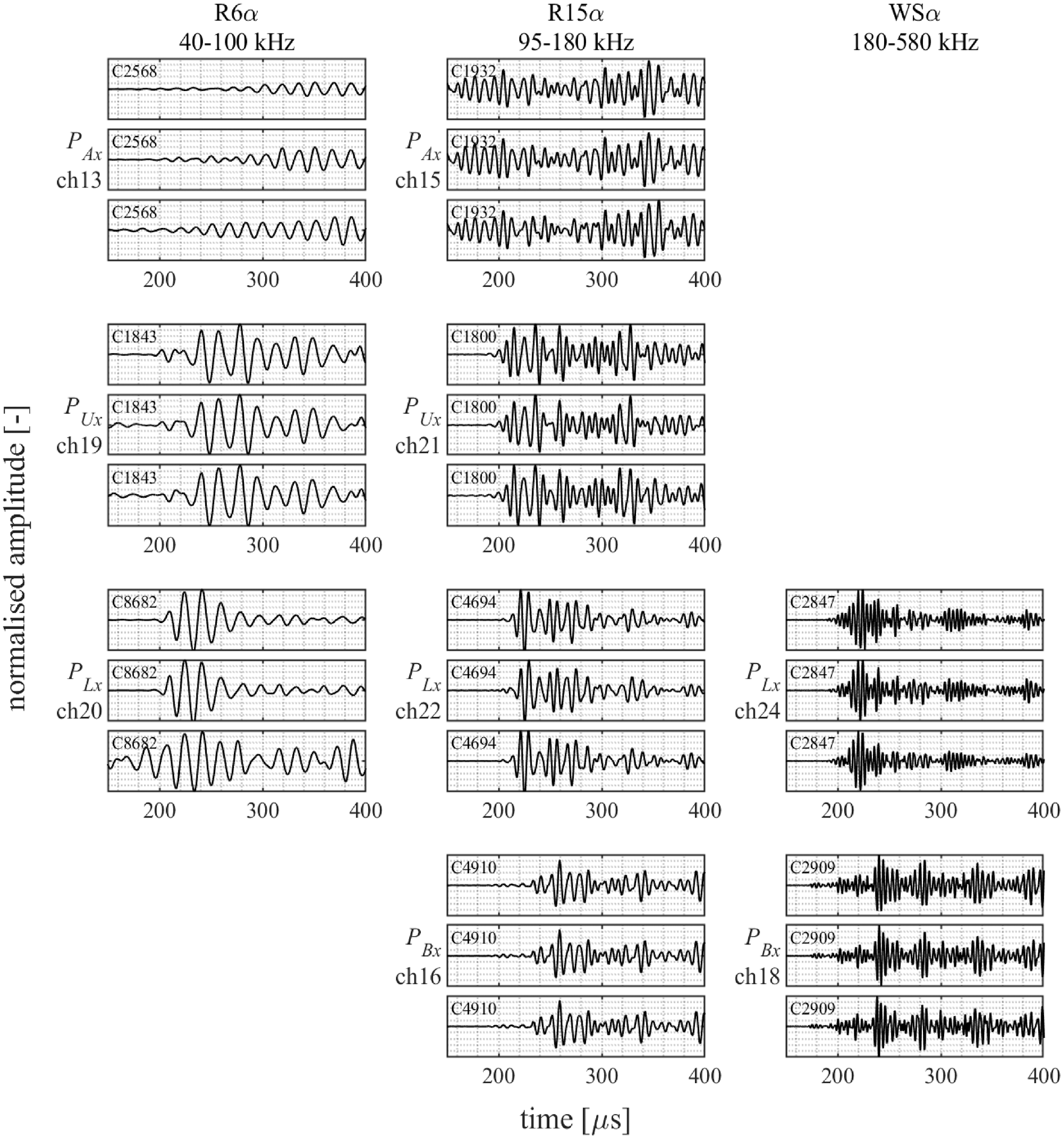
Overview of an arbitrary selection of waveforms associated with the primary structure of clusters.
For some of the measurement channels, the structure is split between multiple clusters. Notable examples – that are also elucidated in Figure 9– are the selected clusters for channels 19 and 20. In Figure 8, the amplitude trends of the individual hits composing these clusters clearly match the overarching trend; however, in Figure 9, the waveforms are shown to contain some minor differences – in particular near the onset – which have likely resulted in a close-miss for the clustering approach. Eventual fine-tuning of the dissimilarity threshold could alleviate this occurrence; however, for the purpose of this study, this is omitted.
In general, the primary structure of clusters seems to comprise two trends. There is a clear line of highly similar hits with amplitudes near equal to the neighbouring hits. This trend seems to be present for a duration of 7,500 cycles, and is detected and clustered for nearly all of the measurement channels. The second trend shows a more cloudy behaviour, with greater variance in the detected peak amplitudes, though waveforms remain highly similar. Overall, amplitudes for the second trend seem less pronounced, and therefore it is detected and clustered to a lesser extend in comparison to the first trend. The second trend is present for a duration of 5,000 cycles, with the onset just before 175,000 cycles.
Focussing on the highly consistent line-shaped trend, the source of the signals and thus the location of the degradation can be derived. The basis for this derivation is the systems of transformations described in Equations (1) through (12). Taking the mid-frequency graph as an example, the greatest amplitudes are detected on the nose raceway (channel 22, cluster 4367) at around 90 dB. On the opposing raceway (channel 21, clusters 1663 and 1674), an amplitude of about 65-70 dB is detected. The difference between these locations is a drop in amplitude of 20–25 dB, that matches the results obtained in earlier work on the relative drop in amplitude for a signal propagating from one raceway to another through a roller. 13 Similarly, the differences between the raceway and substructure channels are shown to be in the order of 5–10 dB. These numbers are slightly better than predicted in the earlier work for a single interface transmission; however, it must be noted those experiments assumed a line contact, whereas the interface between raceway and substructure is a surface.
Comparable differences in amplitudes can also be observed in the low- and high-frequency graphs in Figure 8; however, the roller transmission for the low frequencies seems a bit stronger, at about 20 dB amplitude loss. While the high frequencies show a slightly weaker transmission, at about 30 dB amplitude loss.
Regarding the cloud-like trend observed around 175,000 cycles, it must first be stated that these are the same clusters that comprise the line-shaped trend. This is most obvious when looking at the cluster for channel 22 (cluster 4367 in the middle graph of Figure 8), which contains both the line-shaped trend with the greatest amplitudes among the line-shaped trends, and the cloud-shaped trend with generally the greater amplitudes among the cloud-shaped trends. These being in the same cluster indicates that these seemingly separate trends share highly consistent waveforms, with the only significant difference between them being the consistency of the amplitude. The signals in the line-shaped trend show a minimal and gradual variation in the amplitudes, indicating that the emission mechanism consistently releases similar amounts of energy into the material with each hit. Contrasting to this is the cloud-shaped trend, where the variation in amplitude between the signals indicates a varying amount of energy released into the material for each hit.
Concluding, all of the identified clusters in the largest structure of clusters seem to indicate that degradation is developing in the nose raceway of the top chamber. This degradation is mostly of a highly consistent nature, which might indicate some form of crack propagation.
The secondary structure of clusters, shown in Figure 10, is encountered between 184,400 cycles and 186,400 cycles. An arbitrary selection of three illustrative waveforms from each of the measurement channels comprising this structure of clusters is depicted in Figure 11. The structure is composed of about 13,500 AE hits that are detected by 9 of the 12 sensors. The average similarity of each waveform to its respective cluster is 0.94. The most noticeable averaged activity reaches just upwards of 1 hit per cycle. Comparing this to the hit-rates shown in Figure 5, the clusters in the structure make up about a quarter of the activity during its duration of some 2000 cycles. As was the case with the other structure of clusters, residual activity is likely related to mechanisms emitting less consistent waves.
Secondary structure of selected clusters from low- (top), mid- (middle) and high-frequency (bottom) measurement channels.
Overview of an arbitrary selection of waveforms associated with the secondary structure of clusters.
The individual clusters, that have been selected to compose this structure, all show a clear trend of hits with a consistently increasing and subsequently decreasing amplitude. Using the reasoning introduced earlier regarding interfaces and transmission losses, it is expected that the secondary structure of clusters comprises signals that were generated in the nose raceway, as was the case with the primary structure of clusters. These observations, the similar trend in emission behaviour and the same source component, imply that the degradation responsible for both structures of clusters might be of similar character. Seemingly contradicting is the notion that the separate clustering of the individual hits in both structures of clusters is the result of dissimilarity between the clusters within the structures. However, progressive failure of the rolling elements alters transfer paths and transmission surfaces, and as such deviation of the long-term similarity is expected with increasing damage, while the short-term similarity is retained. Note that separation of larger clusters into several smaller ones may obfuscate the identification of particular types of degradation and is to be further investigated in the future research regarding long-term tracking of particular clusters.
Manual identification of structures in the obtained clusters, as performed prior, is a laborious process, that is also subject to misinterpretation. To circumvent these issues, common techniques for structuring multi-channel AE data, such as event-building, may be implemented. A basic implementation of this combined event and cluster-based filtering is presented in Figure 12. Therein, the global cumulative hit count is shown for all hits that meet the criteria of being associated with (i) a cluster containing at least 100 elements and (ii) an event that has been detected by all of the sensor types and on at least two of the measurement locations individually.
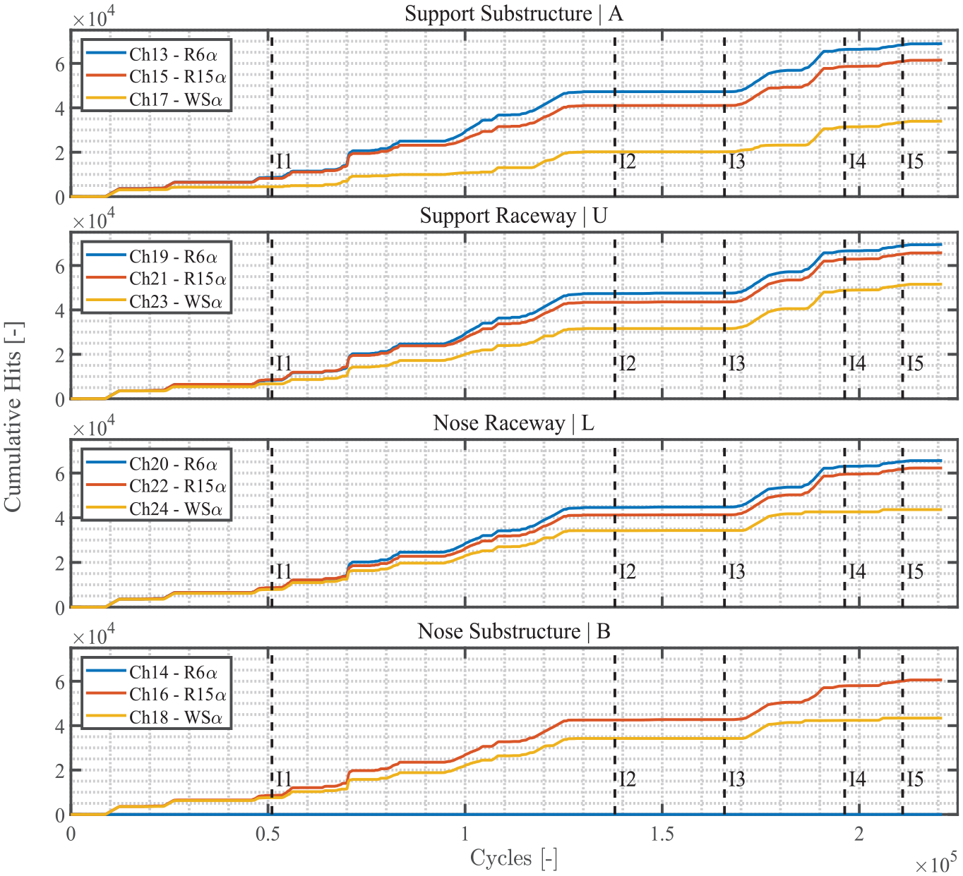
Cumulative hit count in the top chamber filtered for (i) the detectability of the event in both at least three frequency ranges and at least two measurement locations and (ii) the association with a cluster comprising at least 100 elements. The dashed vertical lines (I1–I5) indicate the five performed inspections.
Figure 12 shows four graphs, each representing the three sensor types on a particular measurement location. The visual similarity in the trends is obvious, indicating that most commonly the identified clusters are detectable on all measurement locations. Note that the prescribed association in the event-building procedure does partly impose this similarity in the trends; however, this is limited to a fraction of the measurement channels. The overall similarity in the trends indicates the feasibility of condition monitoring on the basis of propagated signals.
The trends in all four graphs of Figure 12 show the major rises in the cluster-event filtered cumulative hit count to be occurring between the first (I1) and second (I2) inspection, and between the third (I3) and fourth (I4) inspection. The monitoring results from both of periods comply with the observations of increased wear. Considering the structures of clusters shown in Figures 8 and 10, the two separately identifiable increases in hit count between I3 and I4 are associated with the structures presented in those respective figures. However, the continuation of the later of these increases till around 190,000 cycles indicates that a part of these clusters have gone unnoticed in the manual identification. The same limitation should be extended to the rise in hit count between I1 and I2, of which none of the underlying structures was identified in the manual evaluation. Therefore, this implementation demonstrates the effectiveness of combined clustering and event-building in isolating potentially significant AE activity.
The presented methodology in this article has been supplemented with a complete and extensive data sample covering the entire degradation process of the rolling elements. If fewer data are available, the reliability of the identification approach may be reduced. In future research, the minimum required data sample from which to reliably infer bearing condition is to be investigated. Furthermore, the reported experiments represented a moderately noisy environment. It is recognised that higher-noise environments might exist in practical situations subject to harsh working conditions and thus may require more elaborate noise countering measures. In future work, application of the proposed methodology on representative installations and possible associated challenges in the field will be investigated.
Conclusions
A methodology for identifying degradation in low-speed roller bearings based on similarity of AE source signals and a sequential clustering algorithm based on cross-correlation of recorded AE signals is proposed. The possibility of utilising propagated and transmitted signals instead of source signals is discussed and formulated analytically. To verify the methodology, a natural degradation test has been executed in a representative scale on a purpose-built linear bearing segment modelled after the support bearing of an FPSO turret. Over the course of 225,000 cycles, AEs have been recorded at four locations both on the rolling elements and on the supporting structure by sensor arrays comprising of three AE transducers, each sensitive to a particular part of the covered 40–580 kHz frequency range. The recorded signals have been filtered and clustered, to identify consistent trends and structures that may indicate developing degradation. Analysis of the clustered signals shows an increase in similar emissions around 70,000 cycles that is likely indicative of an increase in the degradation rate. This increased wear development is supported by visual inspections of the rolling elements. Additionally, around 175,000 cycles, two highly consistent structures of clusters have been observed to originate from the nose raceway, which may be indicative of the development of a localised defect in that raceway. These results suggests that (i) clustering based on cross-correlation may be used to identify consistency in AE source mechanisms, (ii) combined clustering and event-building provides an effective method for isolating significant AE activity, (iii) for sufficiently low speed, propagation and transmission of AE signals throughout the rolling elements, interfaces and substructure is governed by (quasi-)static attenuation, and (iv) relative differences between clusters identified for different sensor locations may be used to identify the component the source signal originates from.
Footnotes
Appendix
Acknowledgements
The authors are grateful to Bluewater Energy Services, Sofec and Huisman Equipment for their contribution in engineering and fabricating the test setup. Huisman Equipment is additionally acknowledged for their support during the execution of the tests.
Declaration of conflicting interests
The author(s) declared no potential conflicts of interest with respect to the research, authorship, and/or publication of this article.
Funding
The author(s) disclosed receipt of the following financial support for the research, authorship, and/or publication of this article: This work was supported by the HiTeAM Joint Industry Project partners; and Top consortium for Knowledge and Innovation Maritime (TKI Maritime) of the Netherlands Enterprise Agency (RVO).
Data availability
The data presented in this study are available upon request from the corresponding author.