
Abstract
Structural health monitoring aims for the identification of damage. In order to identify damage using model updating, vibration measurement data is recorded, damage-sensitive features are identified and a numerical model is updated to match the structural behavior observed. However, uncertainty exists in every model updating application in structural dynamics. As established approaches for uncertainty quantification and propagation are dependent on previous assumptions regarding the input data (e.g., modal parameters), in this work, an alternative model updating procedure is proposed, namely the sample-based deterministic model updating (SDMU) approach. The key idea is to decouple the uncertainty incorporation from the actual model updating procedure by combining a sample provision with a numerical optimization algorithm. Using this approach, the uncertainty is incorporated indirectly through the performance of multiple deterministic model updating procedures based on each discrete input sample. The type of sample provision, just as the optimization algorithm, is freely selectable. The performance and adaptability of the proposed SDMU approach are demonstrated using a simple analytical application example and a laboratory steel cantilever beam with the aim of damage identification. Results are compared to the results of a benchmark Bayesian model updating (BMU) method, namely the transitional Markov chain Monte Carlo method. Findings show that the BMU and SDMU outcomes directly reflect their input data, whereby the considered SDMU realizations show a clear and more distinct convergence behavior. This highlights the advantages of the SDMU approach: Adaptability to the problem at hand, independence from assumptions about the input data and correct reproduction of its characteristics.
Keywords
Introduction
In civil engineering, non-destructive damage identification methods are of vital importance when seeking to maintain the safety and integrity of the structures under consideration.1,2 Updating the numerical models is among the most notable vibration-based non-destructive damage identification methods. 3 Within a structural health monitoring framework, the basic assumption is that damage, defined as degradation of the mechanical properties, 4 causes detectable changes in the structural dynamic behavior. 5 Thus, in order to identify damage, vibration measurement data corresponding to at least two different states of the considered structure need to be recorded. Subsequently, damage-sensitive features are identified, and a numerical model is updated to match the structural behavior observed.
Typically, the problem is formulated inversely and can be treated as an optimization problem, as trial-and-error approaches are time-consuming and often not feasible for complex engineering structures.6,7 An objective function is used to compare the structural dynamic behavior of the numerical model to a target (i.e., damaged) state, and an optimization algorithm is used to find a model to match this target state by updating the design variables selected. Most often, this is achieved through stiffness or mass modifications. 8 Usually, in civil engineering applications, output-only measurement setups are installed, and excitation forces are rarely known. This is why measured time domain data are of little use for model updating approaches and the objective function generally comprises the difference between modal parameters or frequency response functions,9,10 identified from the measured data using signal processing and operational modal analysis techniques. 11
Simoen et al. 12 identify that many issues arise due to two major sources of uncertainty affecting the model updating process. One source of uncertainty is the numerical model used in the updating procedure. A numerical model is always an idealization of the structure under consideration, causing an inherent discrepancy between the model predictions and the corresponding characteristics identified from the measured data.9,13 Another source of uncertainty is the recording of measurement data. Due to the inevitable spatial sparsity and noisiness of sensor signals and possible imperfections in the measurement equipment, measured data are always a source of uncertainty, which can merely be minimized but never fully eliminated. 14 In addition to the uncertainty contained in the raw measurement data, further uncertainty is introduced during the subsequent signal processing and extraction of modal characteristics of the physical structure, 8 referred to as identification uncertainty. The identification uncertainty depends on the measurement uncertainty, which is partly passed on, and on the uncertainty regarding the choice and application of the operational modal analysis technique.
The addressed sources of polymorphic uncertainty, comprising aleatory and epistemic components, underline the limitations of purely deterministic model updating approaches as reviewed by Mottershead and Friswell. 5 Their output contains a single optimal design variable set with no information regarding the confidence in this solution or its sensitivity with respect to varying input or model parameters. To achieve a more informed and reliable prediction (i.e., damage identification), methods are essential that incorporate and propagate uncertainty. Ereiz et al. 13 give a comprehensive review of deterministic and stochastic finite element (FE) model updating methods for structural applications. Bi et al. 15 present a thorough overview and step-by-step methodology of stochastic model updating and uncertainty quantification, along with useful definitions. Established approaches for uncertainty quantification and propagation in model updating include the probabilistic Bayesian model updating (BMU) approach, 16 the Monte Carlo (MC) sampling-based approach 17 and non-probabilistic interval or fuzzy approaches. 18 Comparisons between the BMU and the sensitivity-based model updating approaches can be found in Patelli et al. 19 and Bi et al. 20 Govers et al. 21 provide a comparison between two stochastic, non-probabilistic model updating methods based on mean and covariance updating and based on interval updating. Zhang 22 provides a substantial survey of (recently) introduced extensions of the standard MC method, aiming to reduce the computational effort when utilizing more complex numerical models. Naturally, all model updating approaches have their individual advantages and disadvantages. However, a necessary requirement of all these approaches considering uncertainty is that previous assumptions about the input data have to be made when formulating the objective or likelihood or membership function or the variance reduction techniques applied within improved MC-based methods. This represents the motivation for the proposal of an alternative to the addressed model updating approaches.
The approach proposed and presented in this work is based on the combination of a sample provision with a numerical optimization algorithm. The key idea is changing the order of operations regarding the incorporation of uncertainty compared to traditional BMU methods. Instead of directly including the uncertainty within the objective (or likelihood) function formulation, the uncertainty is taken into account indirectly through the evaluation of multiple discrete input samples. Subsequently, multiple deterministic model updating procedures are performed based on each input sample, giving the proposed approach the name sample-based deterministic model updating (SDMU). Using this approach for the model updating of real (including laboratory) structures, input uncertainty in the form of identification uncertainty, including measurement uncertainty, is considered and propagated. The identification uncertainty is mostly aleatory or stochastic but can be minimized to a certain degree by considering longer measurement times. A constant discrepancy between the numerical model and the real structure is accounted for through a relative formulation of the objective function. Model form error caused by the choice of the numerical model is assumed to be zero, as a specific model is set in advance of the model updating application. Consequently, epistemic uncertainty in the form of parametric and model form uncertainty is not inherently incorporated within the SDMU approach but is partly accounted for due to the presented objective function formulation.
Decoupling the incorporation of uncertainty from the model updating procedure itself represents a fundamental difference with respect to BMU methods and a motivating factor and concurrent advantage of the SDMU approach. Regarding this aspect, the proposed SDMU approach shares a conceptual similarity with sampling-based approaches, whereby MC-based methods are typically used for uncertainty propagation in model updating.23–25 However, the key difference is that, using the SDMU approach, both the type of sample provision and the choice of the optimization algorithm are entirely flexible, making the approach fully adaptable to specialized problem formulations. The input samples can either be generated by applying any type of sampling method, including MC sampling or bootstrapping algorithms. Both of these sample generations necessarily involve prior assumptions regarding the distribution of each input parameter. However, as the general SDMU approach separates uncertainty treatment from the objective function formulation, the input samples can also comprise empirically obtained data points without any distributional assumptions. Consequently, the proposed approach is sample-based rather than sampling-based, making it more adaptable and applicable to a wider spectrum of applications. Regarding the choice of the optimization algorithm, any local, global, deterministic, metaheuristic or even multi-objective optimization algorithm can be used with respect to the problem at hand. This interchangeability even allows for the selection of an SDMU realization that is able to provide fully reproducible results. The adaptability of the SDMU approach is a great advantage and useful tool, since the well-known “no free lunch theorems for optimization” 26 clearly state that there can be no method that performs best for every kind of optimization problem.
As multiple evaluations of the objective function are time-consuming, especially when many input samples are present and larger FE models are to be solved, the use of a meta-model is integrated into the SDMU approach. As the set-up procedure is implemented as part of the underlying approach, the coupling to meta-models can be easily achieved.
The following highlights summarize the addressed benefits of the SDMU approach proposed.
Independence of previous assumptions about the input data if empirical data points are utilized due to the decoupling of the uncertainty incorporation from the model updating procedure.
Adaptability to the problem at hand due to the free selection of the type of sample provision and optimization algorithm that make up a specific SDMU realization.
Possibility to choose SDMU realizations that provide deterministic, fully reproducible results.
Effortless coupling to meta-models, as the set-up procedure of the meta-model is integrated into the SDMU approach.
In this work, two levels are addressed. The first level is to motivate and propose the general SDMU approach, considering uncertainties. The second level comprises the actual application of the proposed procedure. To achieve this, of course, a specific sample provision and a specific optimization algorithm need to be chosen. Using the analytical application example in section “Analytical example: two-degree-of-freedom system,” a variety of possible SDMU realizations is investigated. Random and quasi-random sampling methods are introduced, as well as a data point-based approach without the need for prior assumptions regarding the input parameter distribution. In addition, different deterministic and metaheuristic optimization algorithms are applied. Subsequently, one of the presented fully deterministic SDMU realizations is chosen for the application to the model updating of a laboratory steel cantilever beam with the aim of damage identification in section “Experimental validation: laboratory steel cantilever beam.”
In the course of each application, the results obtained using the different SDMU realizations are compared to the results of an established representative BMU method using the well-known transitional Markov chain Monte Carlo (TMCMC) sampling technique. Although the BMU and the proposed SDMU approach are not directly comparable in principle, both approaches were applied under equivalent conditions and identical assumptions regarding model parameters and design variable configuration. This ensures that the propagated input uncertainty is consistent, and a comparison of the results is meaningful.
Theory
Figure 1 gives a schematic overview of the different essential steps for model updating considering uncertainty using the SDMU and BMU approach. First of all, naturally, measurement data need to be recorded for the structure under investigation. Subsequently, the identification of specific features from the raw measurement data, including a quantification of the inherent uncertainties, is necessary for all model updating methods considered. In this work, modal properties
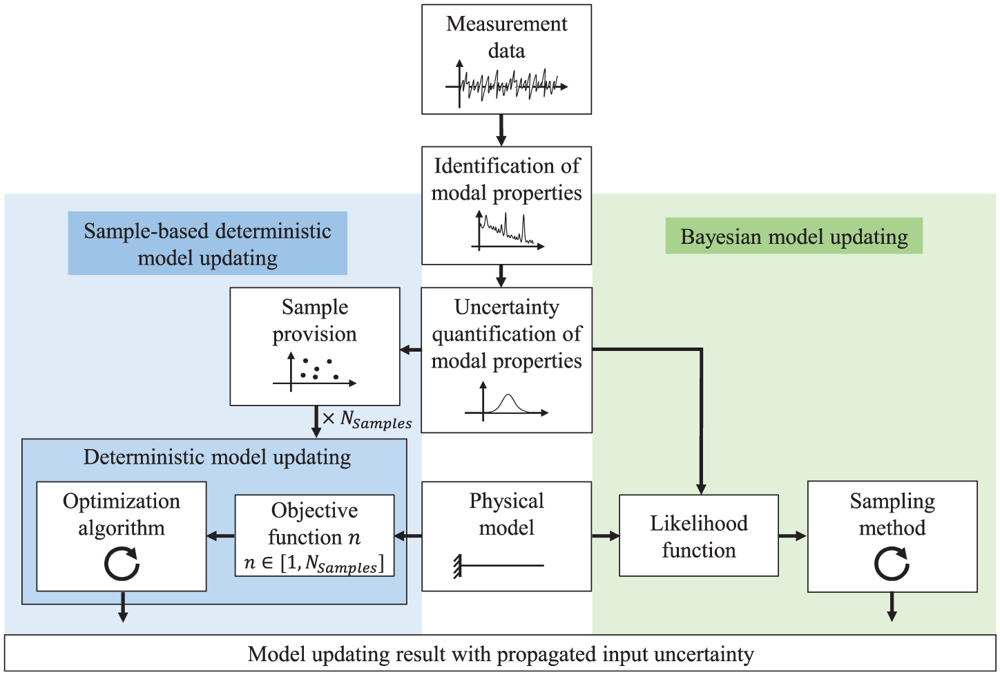
Schematic overview of the essential steps for model updating considering uncertainty using the SDMU or BMU approach.
As depicted in the flow chart in Figure 1, the main difference between the two model updating approaches SDMU (left, blue color) and BMU (right, green color) lies in the handling of the uncertain input and the formulation of the objective function. Whereas the objective function of BMU methods, also called the likelihood function, incorporates the uncertainty explicitly, the SDMU approach includes the uncertainty implicitly through the evaluation of multiple independent objective functions. In the following, the fundamentals of the two model updating procedures applied and compared in this work are outlined in detail. The descriptions focus on dealing with uncertain values in the objective or likelihood function formulation.
Every model updating method represents an optimization method, essentially designed to solve scalar, bounded and nonlinear optimization problems

where

where
Bayesian model updating
A possible way to explicitly incorporate quantified identification uncertainty into the model updating procedure is to use Bayesian inference based on Bayes’ theorem30,31
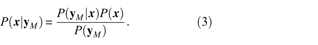
In this case, the posterior distribution
Several different advanced sampling methods can be used to incorporate the occurring uncertainties into the BMU procedure, as depicted in Figure 1. For this work, the well-established TMCMC algorithm developed by Beck and Au
32
and Ching and Chen
33
is considered as a sampling method. It utilizes transitional probability density functions
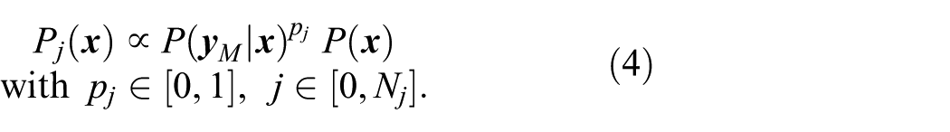
Here,
Objective function formulation
For each sample, the objective or likelihood function is evaluated. In this work, the formulation of the likelihood function is based on the assumption of a log-normal distribution with mean values
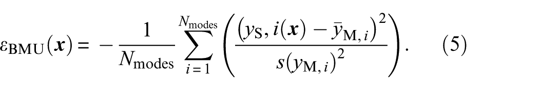
The subscript
Sample-based deterministic model updating
The motivation behind the SDMU approach is to reverse the order of operations regarding the incorporation of the identification uncertainty compared to traditional BMU methods. Specifically, the uncertainty is excluded from the objective function formulation. Consequently, instead of an explicit incorporation entailing assumptions about the input data, the uncertainty is taken into account implicitly within the SDMU approach. This is achieved by using multiple discrete input samples (in this work, modal parameters), which may either be generated using any kind of sampling method or bootstrapping algorithm—requiring assumptions about the input data—or may be directly available as empirical data points—requiring no assumptions about the input data. Subsequently, multiple separate deterministic model updating procedures are performed for each input sample using a numerical optimization algorithm. Similar to the choice regarding the sample provision, the choice of the optimization algorithm is arbitrary. This interchangeability of the type of sample provision and the choice of the optimization algorithm represents one of the key advantages associated with the SDMU approach because it makes the approach fully adaptable to the specific problem at hand. It also allows certain SDMU realizations to be selected in such a way that they deliver fully reproducible results. The SDMU approach and its fundamental difference compared to the BMU approach regarding the incorporation of uncertainty are depicted in Figure 1.
Objective function formulation
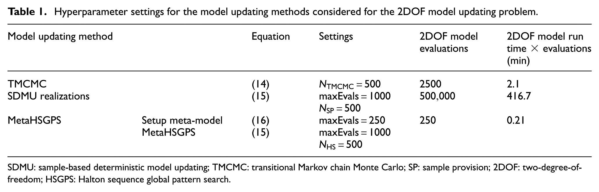
In this work, a number of
The input for the model updating procedure is now an
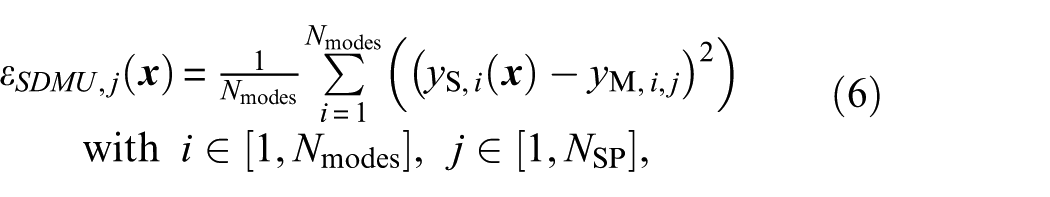
where the subscript
Sample-based deterministic meta-model updating (metaSDMU)
For high sample numbers and more complex numerical models, the SDMU approach will eventually become computationally very expensive (cf. Equation (6)). This challenge is well-known from (MC) sampling-based uncertainty propagation methods, where extensive research focuses variance reduction techniques and enhanced sampling strategies. 22 This is why, in this work, the use of a surrogate or meta-model is proposed to reduce computational effort. This approach is called sample-based deterministic meta-model updating, or metaSDMU.
The idea is to derive a meta-model using a single deterministic model updating procedure based on the mean of each uncertain value

This way, the potentially computationally expensive model evaluations required in every iteration step only have to be performed during one model updating procedure. Otherwise, the model updating with consideration of uncertainty is performed using the meta-model, which is computationally much more efficient.
For both application examples presented in this work, the natural neighbor interpolation is chosen, which represents a multi-dimensional linear interpolation approach for scattered data. 35 The reason for this choice is that this meta-model was found to be sufficient for the two particular model updating problems while being very simple. It reproduces the exact values of the training data and requires no tuning of hyperparameters. Furthermore, the natural neighbor approach can easily be scaled to higher-dimensional applications. A disadvantage of the natural neighbor interpolation is that, due to its linearity, salient points appear at the training data points, and curved surfaces can only be approximated adequately if sufficient training data is available. However, this requirement is met as the use of one representative deterministic model updating procedure generates a sampling pattern within the design variable space (i.e., the training data), which is dense in the area where the optimal solution(s) are expected. Of course, a variety of other choices for the meta-model are also possible and, naturally, the best choice depends on the problem at hand. More advanced meta-modeling methods, like the well-known Gaussian processes, for example, would have required choosing a kernel function, making the meta-model setup more complicated.
The relative ease, with which the SDMU approach proposed can be coupled to meta-models represents another benefit, facilitated by running the deterministic model update on the mean values of the uncertain quantities and using the evaluated points to populate the meta-model. In this work, a meta-model is only set up for the SDMU approach, as the set-up procedure is already part of the underlying model updating approach. To be fair, any BMU method could also be employed on a meta-model, and the number of model evaluations would be reduced to those necessary for its setup. However, the aim of this work is not to compare the number of model evaluations but to introduce the SDMU approach and to compare the results of representative SDMU realizations with the TMCMC method, representing a benchmark BMU (sampling) method often used in literature.
Analytical example: two-degree-of-freedom system
The two model updating approaches SDMU and BMU considered in this work are verified and compared using a simple two-degree-of-freedom (2DOF) system often used in literature.34,36 Such a minimal benchmark provides a transparent environment in which the fundamental characteristics of each method can be isolated, validated, and understood. This is an essential, necessary basis for subsequent applications to more realistic, higher-dimensional structures.
A sketch of the 2DOF system is shown in Figure 2. The aim of this model updating problem is to identify the correct spring stiffnesses
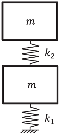
Sketch of the 2DOF system.
Design variables and objective function formulation
The linear spring stiffnesses

which parameterize the stiffness matrix
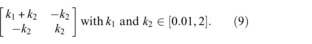
Both masses are set to
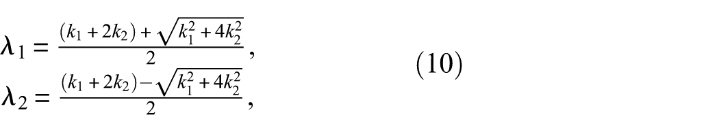
such that
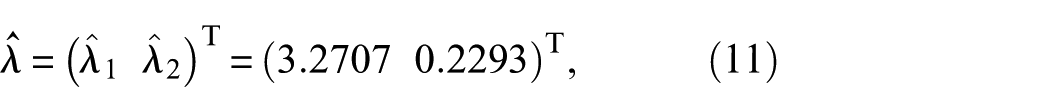
with the hat denoting correct values. The correct stiffness values within the given bounding vector, again denoted by a hat, are
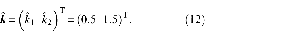
The “measured” (i.e., noisy) eigenvalues are randomly generated according to a Weibull distribution with the shape parameter selected to
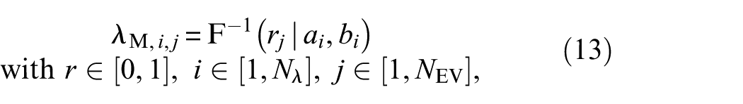
where the subscript

Illustration of 500 generated eigenvalue samples using a Gaussian and a Weibull distribution function, respectively, with highlighted corresponding mean values and standard deviations.
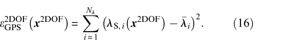
In the following, the objective functions for the different model updating approaches considered are given. The objective (or likelihood) function used within the BMU approach is defined as
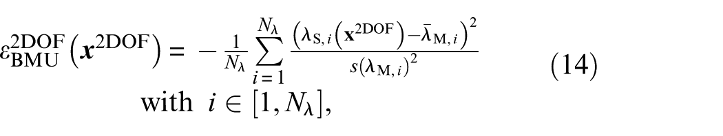
whereby
While the objective function of the BMU approach (cf. Equation (14)) incorporates the uncertainty explicitly by integrating the mean eigenvalues
Application
Using the 2DOF model updating problem, two possible sample provisions used within the SDMU approach are presented in detail. Firstly, a data point-based sample provision is investigated to demonstrate the possibility of the SDMU approach being completely independent of previous assumptions about the input data (advantage No. 1 in the section “Introduction”). Secondly, a variety of SDMU realizations employing random and quasi-random sampling methods are applied and compared using the 2DOF model updating problem to demonstrate the easily facilitated adaptability of the SDMU approach (advantage No. 2 in the section “Introduction”). The sampling methods are respectively combined with different deterministic and metaheuristic optimization algorithms. Furthermore, within this investigation, several SDMU realizations are introduced that provide fully deterministic results (advantage No. 3 in the section “Introduction”). In addition to the demonstration of different sample generations based on sampling methods, the use of a meta-model within the metaSDMU approach is presented (advantage No. 4 in the section “Introduction”). In all cases, the results of the SDMU realizations are compared to the results obtained using the TMCMC algorithm, chosen as a benchmark BMU sampling method.
Before the model updating scheme is employed, convergence studies were performed to find appropriate settings for the hyperparameters of the model updating methods presented. The findings regarding the hyperparameter settings, including the number of samples and the maximum number of objective function evaluations, are presented in detail in Appendix A.
Sample provision based on data points
Regarding damage-sensitive features identified from the measurement data, oftentimes no distinct distribution is available but rather few discrete values are on hand. This is why this subsection presents a practice-oriented case of application, where the SDMU approach is based on a few available data points and, thus, free of prior assumptions regarding the input data. For this task, five eigenvalues are randomly generated similar to Equation (13) from the Weibull distribution function introduced in section “Design variables and objective function formulation.” Subsequently, these five eigenvalues represent the available input samples, that is, possibly experimentally gained data points.
Regarding the BMU approach, the objective function formulation comprises the mean value and standard deviation of the input data (cf. Equations (5) and (14)). As the likelihood function formulated in Equation (14) is based on the assumption of a Gaussian distribution, these characteristic values
Regarding the SDMU approach, the
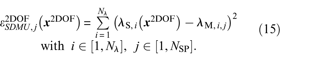
In Figure 4, the optimal eigenvalues and corresponding design variables obtained by both model updating methods TMCMC and DPGPS are shown. For the sake of visibility, only the first of the three runs using the TMCMC algorithm is illustrated here. In addition, the calculated new standard deviation
Comparison of the eigenvalues and corresponding design variables calculated by the TMCMC and DPGPS algorithms for the 2DOF model updating problem based on five data points, representing independent empirically obtained values. The results are shown with respect to the correct solution for each data point and its standard deviation. (a) Eigenvalue space. (b) Design variable space.
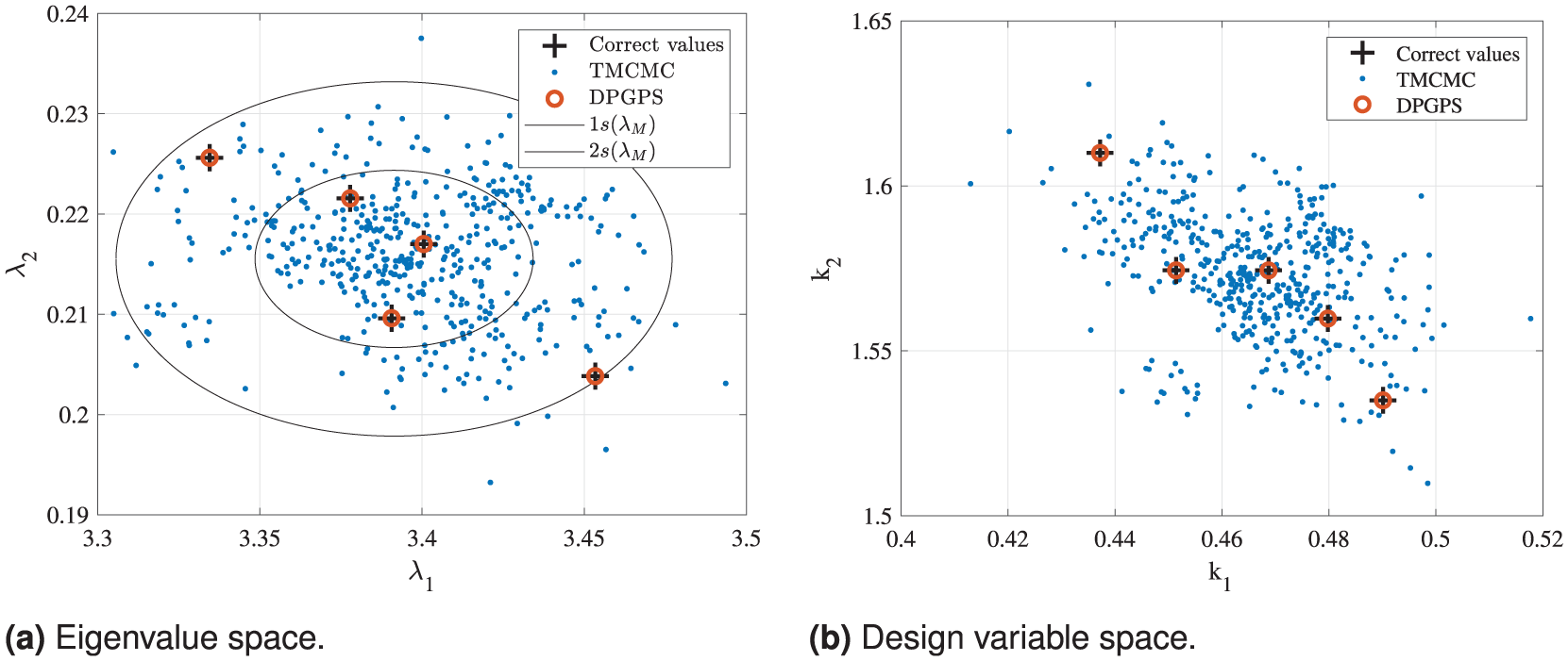
Comparison of the CDFs calculated by the TMCMC and DPGPS algorithms for the 2DOF model updating problem based on five data points, representing independent empirically obtained values. The results are shown separately for the two design variables in addition to the correct solution for each data point. The legend applies to both sub-figures. (a) Design variable
In Figure 4, it is clearly visible that the DPGPS algorithm is able to obtain the five exactly correct solutions regarding the eigenvalues and, thus, also the corresponding design variables. Looking at the CDFs obtained by the DPGPS algorithm in Figure 5, even the same occurrence probability is allocated to each solution. The reason for this distinct solution finding is that the input data simply are the five input eigenvalue samples without any further assumptions or adjustments. For each of these five input data points, a full model updating procedure is performed and a respective clear convergence towards the optimal correct eigenvalues and design variables is achieved. In contrast, the 500 eigenvalue samples and corresponding design variables of the last iteration of the TMCMC algorithm only mirror the approximated distribution of the input data (i.e., the input eigenvalue samples) correctly. However, the exact solutions are not distinctly found but, instead, are located within the solution point cloud or, more precise, within
All in all, these findings clearly underline that the results of the respective model updating methods directly reflect their input data. The DPGPS algorithm, representing the SDMU approach proposed, directly and correctly reproduces the data points given as input. In contrast, the TMCMC algorithm, representing a benchmark BMU method, reproduces the mean value and standard deviation of the input data points. These characteristic values are used as input in the likelihood function based on the assumption of Gaussian-distributed input data.
Sample generation based on a distribution function
To demonstrate the interchangeability and, thus, the adaptability of the SDMU approach (advantage No. 2 in the section “Introduction”), a variety of different random and quasi-random sampling methods and different deterministic and metaheuristic optimization algorithms are applied to the 2DOF model udpating problem. Namely, the random-based MC sampling method
38
and the two quasi-random sampling methods Sobol sequence
39
and Halton sequence (HS)
40
are respectively combined with the deterministic optimization algorithm GPS
37
and the two metaheuristic optimization algorithms genetic algorithm (GA)
41
and evolution strategy (ES).
42
The metaheuristic optimization algorithms are applied using their standard settings and the number of tracked globally best coordinates of the GPS algorithm is set to
The objective or likelihood function of the TMCMC algorithm (cf. Equation (14)) requires the calculation of the mean value and standard deviation from a number of
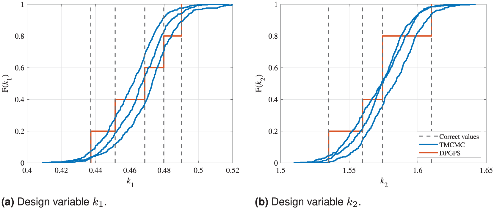
Using the respective SDMU realizations, a sample generation prior to the model updating procedure(s) itself is performed based on the input distribution function using different sampling methods. According to the findings in Appendix A, the number of samples for all sampling methods, including the TMCMC algorithm, is set to 500, and the maximum number of objective function evaluations is set to 1000 for all optimization algorithms. The utilized settings are also listed in Table 1, including a comparison of the 2DOF model run time, which is approximately 0.05 s, multiplied by the required number of model evaluations without accounting for parallelization.
Hyperparameter settings for the model updating methods considered for the 2DOF model updating problem.
SDMU: sample-based deterministic model updating; TMCMC: transitional Markov chain Monte Carlo; SP: sample provision; 2DOF: two-degree-of-freedom; HSGPS: Halton sequence global pattern search.
Figure 6 shows the resulting CDFs of the different SDMU and BMU methods applied to the 2DOF system. As the TMCMC algorithm, the MC sampling method and the metaheuristic optimization algorithms GA and ES are random-based, three runs are calculated per model updating method, including these methods to account for possibly varying convergence behavior. In addition, the correct results regarding the two design variables are indicated using a dashed black line.
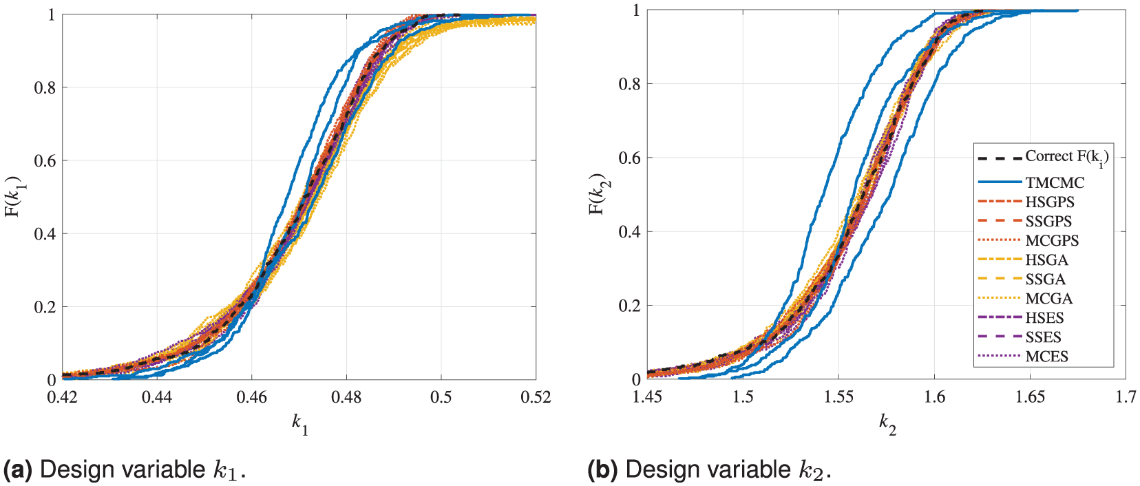
Comparison of the CDFs calculated by the TMCMC algorithm and the nine SDMU realizations for the 2DOF model updating problem based on a Gaussian distribution function and settings provided in Table 1. The results are shown separately for the two design variables in addition to the correct solution. The legend applies to both sub-figures. (a) Design variable
Generally, it can be observed that all applied model updating methods are able to obtain the correct solution regarding the two design variables
In summary, the results illustrate the flexibility of the proposed SDMU approach. Different combinations of sampling and optimization algorithms yield equivalent results, whereby the difference between applying varying SDMU combinations is lower than the scatter between the different TMCMC runs.
Sample-based deterministic meta-model updating (metaSDMU)
For more and more complex numerical models and high numbers of samples, the general SDMU approach will eventually become computationally very expensive (cf. Table 1). This is why, in this work, the use of a meta-model is proposed to reduce computational effort. For this investigation, the same sample generation based on the Weibull distribution function introduced in section “Design variables and objective function formulation” is utilized, and a specific SDMU realization is selected, composed of the quasi-random HS sampling method and the deterministic GPS optimization algorithm, subsequently called HSGPS.
The meta-model, in this case, needed for the metaHSGPS algorithm, is set up using a natural neighbor interpolation of the design variable samples
According to a detailed evaluation of the settings used for the meta-model setup in Appendix section “A.3. Number of samples for the sampling methods within the SDMU approach,” the number of tracked globally best coordinates is set to
Subsequently, for the model updating of the 2DOF problem using the metaHSGPS algorithm, the objective function formulated in Equation (15) is used. In this case, the simulation of each eigenvalue
In the case of the TMCMC algorithm, the number of 2DOF model evaluations depends on the number of iteration steps needed for the algorithm to converge. For this particular problem, five iterations are needed, resulting in
For this rather simple two-dimensional, single-objective analytical model updating example, the effort for the calculation of the meta-model is not really necessary from a computational performance standpoint. The computing time to solve the 2DOF system is very low, so both the TMCMC algorithm and all SDMU realizations are fully practicable. However, for more complicated problems like the solving of large FE models, the setup of a meta-model can save considerable computing effort.
Figure 7 shows a comparison of the CDFs resulting from the use of the three methods TMCMC, HSGPS, and metaHSGPS. Again, the correct results regarding the two design variables are indicated using a dashed black line.
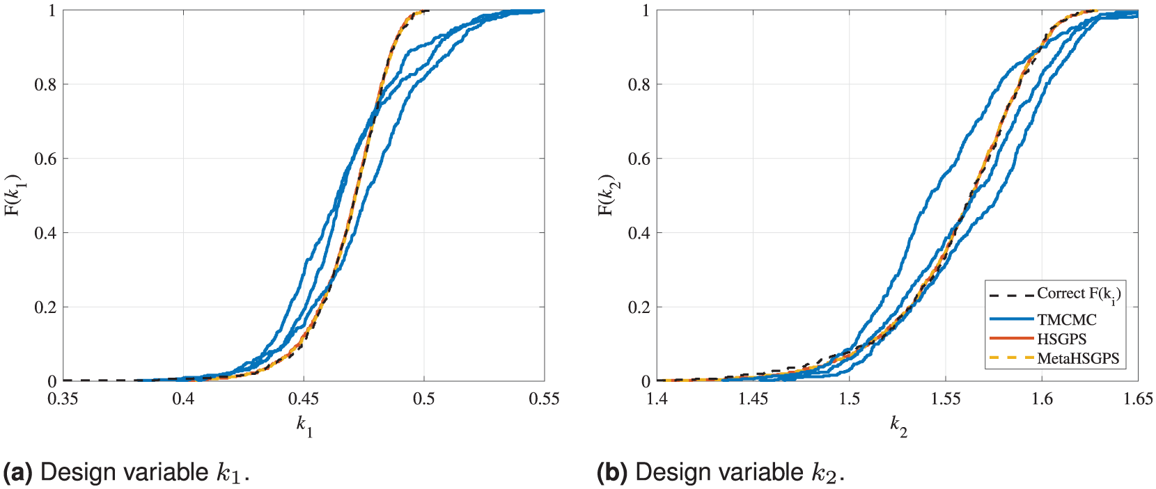
Comparison of the CDFs calculated by the TMCMC, HSGPS and metaHSGPS algorithms for the 2DOF model updating problem based on a Weibull distribution function and settings provided in Table 1. The results are shown separately for the two design variables in addition to the correct solution. The legend applies to both sub-figures. (a) Design variable
At first sight, all three model updating methods considered perform similarly on the 2DOF model updating problem with artificially introduced measurement noise, which shows that all three methods are well suited to quantify the (in this case simulated) uncertainty. However, the HSGPS and metaHSGPS algorithms are able to nearly exactly map the correct, skewed CDFs of the two design variables due to the Weibull-distributed input data. In contrast, the TMCMC algorithm shows some scatter between the different runs and a slightly different course regarding the CDFs. This underlines the different assumptions regarding the input data. As the input of the TMCMC algorithm is the calculated mean value and standard deviation of
In Figure 7, it is prominent that the results obtained by the HSGPS and metaHSGPS algorithms lie exactly on top of each other. On the one hand, this illustrates that the combination of a quasi-random sampling method and a deterministic global optimization algorithm provides fully deterministic results. On the other hand, the results demonstrate the easily facilitated and precise integration of meta-models. The use of the meta-model does not change the outcome of the model updating procedure in any way—except, of course, when random sampling would be applied.
In summary, in this subsection, the easily facilitated interchangeability of the SDMU approach proposed (advantage No. 2 in the section “Introduction”) was demonstrated by comparing a variety of different SDMU realizations in Figure 6. Furthermore, the possibility to utilize a fully deterministic implementation of the SDMU approach (advantage No. 3 in the section “Introduction”) was pointed out in Figure 6 and, especially, in Figure 7. Both figures also indicate that the selected SDMU realizations are able to obtain more precise results regarding the distribution of the input data compared to the benchmark BMU method using the TMCMC sampling technique. In addition, the results of all SDMU realizations show lower scatter than the results of different TMCMC runs using the same characteristic input values, that is, mean value and standard deviation of the input data. Lastly, the inherent and, thus, easily facilitated integration of meta-models within the SDMU approach (advantage No. 4 in the section “Introduction”) was illustrated in Figure 7, where the results show no variation between the selected SDMU and metaSDMU realization.
Experimental validation: laboratory steel cantilever beam
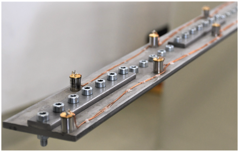
The steel cantilever beam considered is a modular setup of a central beam structure with nine screwed-on fishplates. The fishplates are used to implement a variable, reversible damage mechanism. A schematic overview and a photograph of the modular beam structure are shown in Figures 8 and 9.
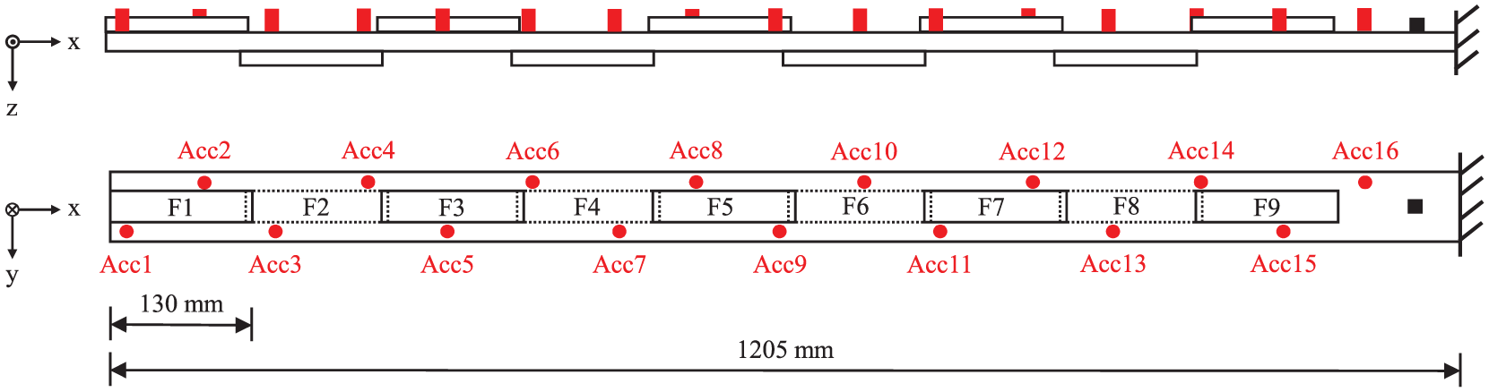
Schematic overview of the steel cantilever beam with nine screwed-on fishplates F1 to F9, including sensor positions (red points) and the position of excitation (black square).
Photograph of the steel cantilever beam.
This modular steel cantilever beam provides a realistic yet controllable structural configuration, allowing the introduction and quantification of well-defined damage scenarios while maintaining experimental repeatability. Such a setup not only increases the complexity beyond the simple 2DOF benchmark system, presented above, but also offers a platform for thorough method validation under conditions that closely mimic real engineering structures. The experimental setup, design of experiments and measurement system utilized are explained in detail in Wolniak et al. 43 The measurement data and the eigenfrequencies and mode shapes identified using BayOMA have been uploaded (separately) to a public data repository of the Leibniz University Hanover.44,45
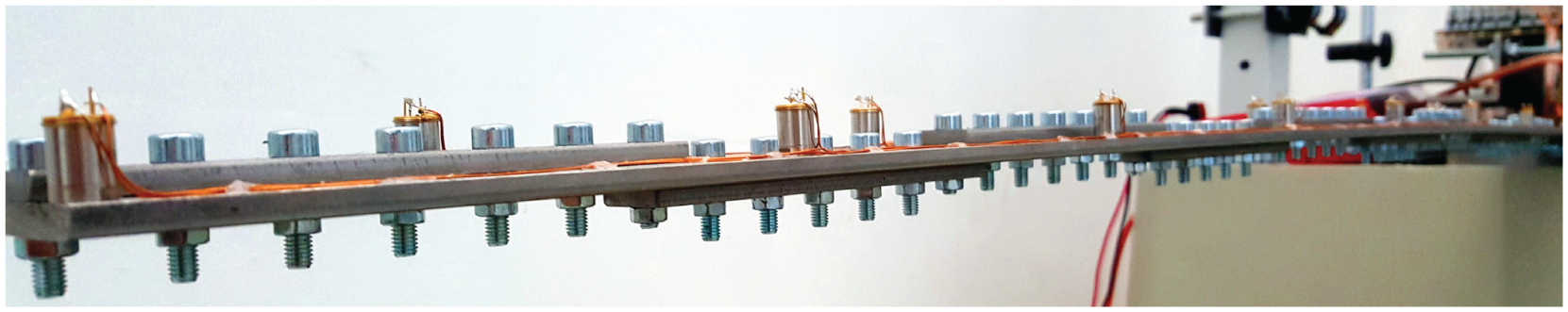
The central beam and the screw-on fishplates are fabricated from rectangular stainless-steel bar stock. As depicted in Figure 8 and visible in Figure 9, the fishplates are screwed on in alternating positions above and below the central beam structure with an overlap of 10 mm. The M5 screws utilized have a uniform separation of 20 mm, yielding a total of 60 screws to connect the fishplates to the center line of the central beam. Thus, each fishplate is held in place by seven screws, whereby the overlapping fishplates share one screw at each respective end. To ensure a repeatable fishplate connection stiffness, the screws are tightened with a consistent assembly torque of
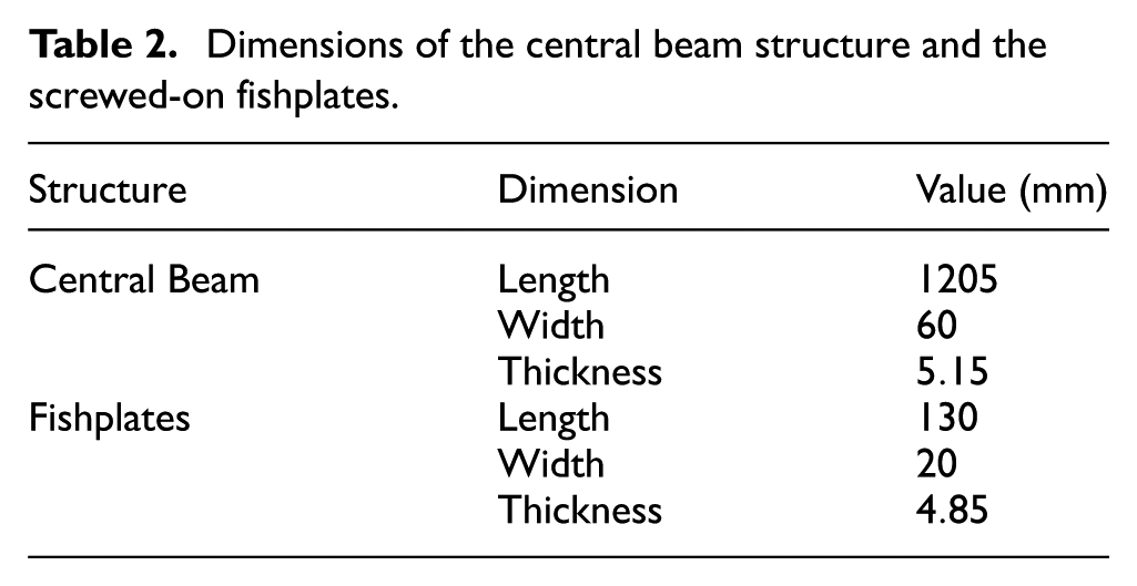
Dimensions of the central beam structure and the screwed-on fishplates.
Close-up of the tip of the laboratory steel cantilever beam.
The central beam with nine undamaged screw-on fishplates represents the reference state of the experiment. The reversible damage mechanism is activated by swapping the intact fishplates for damaged fishplate specimens. Due to the screw-on mechanism, damage can be activated and deactivated without causing permanent alterations to the structure or the fishplates. The damaged fishplate specimens were weakened by sawing cuts into them, which locally reduced their cross-section. In this work, only one damage scenario is considered in detail, namely the uniformly distributed damage. Results of the application of the model updating methods to the two other possible damage scenarios, namely the discrete and Gaussian distributed damage scenarios (cf. Wolniak et al. 43 ), are included in Appendix sections “B.2. Gaussian distributed damage scenario” and “B.3. Discrete damage scenario. ”Figure 11 shows a photograph of the damaged fishplate considered in detail in this work.
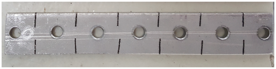
Photograph of the fishplate with the uniformly distributed damage.
The associated measurement series involves sequentially installing the damaged fishplate specimen onto all nine fishplate positions. Before the measurement of each damaged state is recorded, the reference state is restored, and a measurement of the intact state is conducted. Every measurement comprises 1
In summary, even though great attention was given to achieving the same conditions for all measurements, there were some influences that affected the measurements. As the experiment was conducted over several weeks, small changes in the environmental conditions occurred at the experimental site over this time period. The experiment was conducted in a laboratory environment subject to temperature changes and other ambient influences. Vibrations induced by other operating machinery or minor disturbances, such as people passing the experiment, were transmitted through the laboratory floor and affected the measurements. Additionally, several scientists were involved in the execution and recording of the measurements, resulting in slight differences in the screw-on mounting of the fishplates or the adjustment of the shaker excitation. The measurement setup, the setup of the recording measurement system and the method of extraction of the modal data remained identical throughout the whole experiment.
Figure 12 illustrates an example frequency spectrum for the laboratory steel cantilever beam in its reference state, subject to broadband white-noise excitation with highlighted frequency ranges utilized for the BayOMA. For the subsequent model updating procedure, only the first four eigenfrequencies relating to pure vertical bending mode shapes are used. These correspond to the first, second, third, and sixth frequency ranges marked in Figure 12. The measurement time used for the application of BayOMA is chosen to be TData = 30 s. This is a rather short time period considering the general assumption that the longer the measurement time, the less uncertain the results. 46 However, as the aim of this work is to show that the SDMU approach proposed is able to process uncertain input data, the short time period is chosen on purpose. To further explain this choice, a comparison of example model updating results using TData = 30 and TData = 600 s is included in section “Application.”
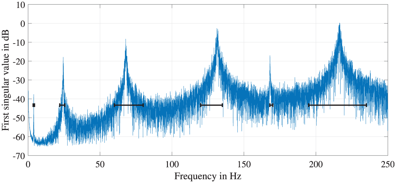
Frequency spectrum of the laboratory steel cantilever beam in the reference state subject to broadband white-noise excitation.
A beam model provides the reference model for the intact steel cantilever beam and is used as the basis for the subsequent FE model updating procedure. A detailed description of the FE model utilized in this work is given in Wolniak et al. 43 The simulations are conducted using the FE analysis software Abaqus.
Design variables and objective function formulation
As damage manifests itself as a change in stiffness, the general approach for most FE model updating procedures with the aim of damage identification is to alter the stiffness properties of the model at hand. 8 This approach is also applied in this work. The utilized parameterization of the design variables was already introduced and successfully employed in several preceding publications.43,47,48
As no prior knowledge of the defect location is assumed for the procedure proposed, the updating of the stiffness properties of all

The stiffness scaling factors

In the design variable vector
Here, the term
The particular associations of the design variables corresponding to the Gaussian damage distribution function are depicted in Figure 13 for the example design variable vector xBeam = (0.4m0.1m0.025) T. More detailed information regarding the damage distribution function can be found in Refs.43,47,48
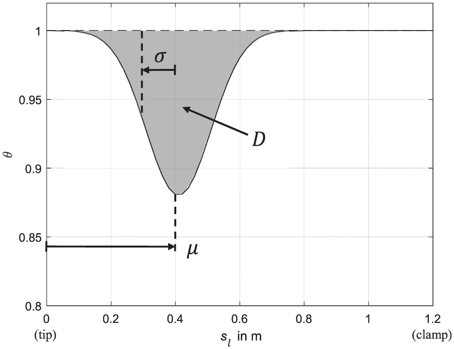
Affiliations of the three design variables demonstrated for the example design variable vector xBeam = (0.4 m 0.1 m 0.025)T for the Gaussian distributed damage distribution function.
In the following, the objective functions for the BMU approach, using the TMCMC sampling technique, and the SDMU approach, represented by the metaHSGPS algorithm, are specified. The basic HSGPS algorithm is not applied to the laboratory structure. As the FE model of the steel cantilever beam is utilized, the application of the HSGPS algorithm is not considered justifiable in terms of computing time. In addition, the previous application of these two specific SDMU and metaSDMU realizations in section “Sample generation based on a distribution function” served to demonstrate that their results stay exactly the same, even when a meta-model is applied.
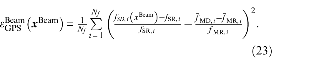
In Wolniak et al., 43 a relative formulation of the objective function is introduced. Using this formulation, a constant initial discrepancy between the simulation and measurement reference states can be suppressed numerically. In addition, the eigenfrequencies of the simulated and measured states are normalized by their reference states to ensure that each eigenfrequency is weighted equally in the objective function. This relative formulation is also employed in this work, and the formulation of the objective (or likelihood) function of the BMU approach based on Equation (5) is adapted accordingly
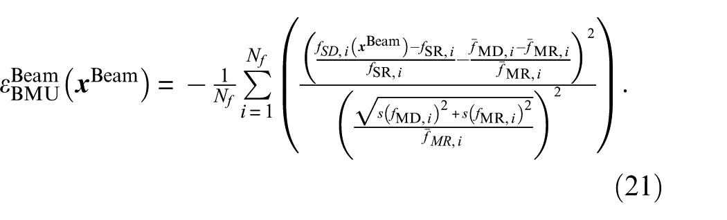
As a result, Equation (21) differs from the original objective function, which is based on a zero-mean Gaussian distribution function.
34
The eigenfrequencies
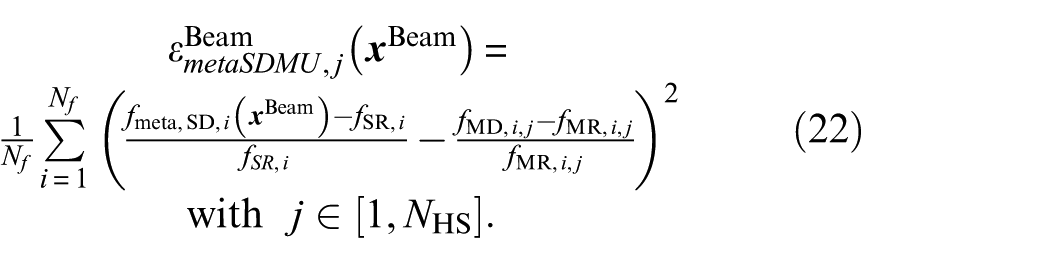
The meta-model used for the metaHSGPS algorithm is set up using the natural neighbor interpolation already employed within the analytical application example in section “Sample generation based on a distribution function.” Input and output are the design variable samples
In all objective function formulations, the design variable vector
Application
Prior to the application of the model updating methods considered, the effect of different eigenfrequencies identified using BayOMA based on different measurement times is demonstrated. Figure 14 shows a comparison of the CDFs of the TMCMC and metaHSGPS algorithms for the design variable
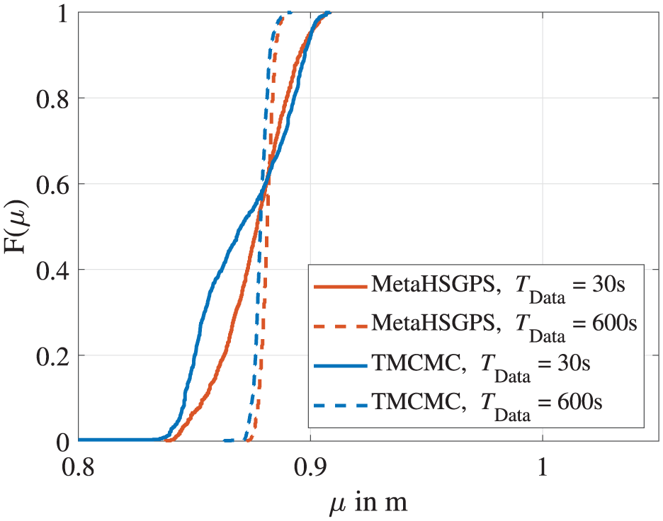
CDFs calculated by the TMCMC and metaHSGPS algorithms for the model updating of the laboratory steel cantilever beam with the damaged fishplate at position F8. The input data comprises eigenfrequencies identified using different measurement times
As expected, it can clearly be seen that the results based on the eigenfrequencies using TData = 600 s (dashed lines) exhibit more confidence than the results based on the eigenfrequencies using only 30 s of measurement time (solid lines). This visually emphasizes the general statement that longer measurement times entail less uncertainty in the modal properties identified using operational modal analysis techniques. 46 As the aim of this work is to demonstrate the handling of uncertain input data, the short measurement time of TData = 30 s is chosen deliberately for the application of the model updating methods considered.
Regarding the hyperparameter settings of the TMCMC and metaHSGPS algorithms, convergence studies are carried out to demonstrate that appropriate settings are utilized. These convergence studies are conducted, similar to the ones investigated for the analytical application example and can be found in Appendix section “B.1. Hyperparameter settings.” The found settings used for the subsequent comparison of the two model updating methods are listed in Table 3, including the necessary number of FE model evaluations needed by each algorithm to solve the model updating of the laboratory steel cantilever beam. In addition, a comparison of the FE model run time, which is approximately 30 s, multiplied by the required number of model evaluations, is included without accounting for parallelization.
Settings for the model updating methods considered for the model updating of the laboratory steel cantilever beam with the aim of damage identification.
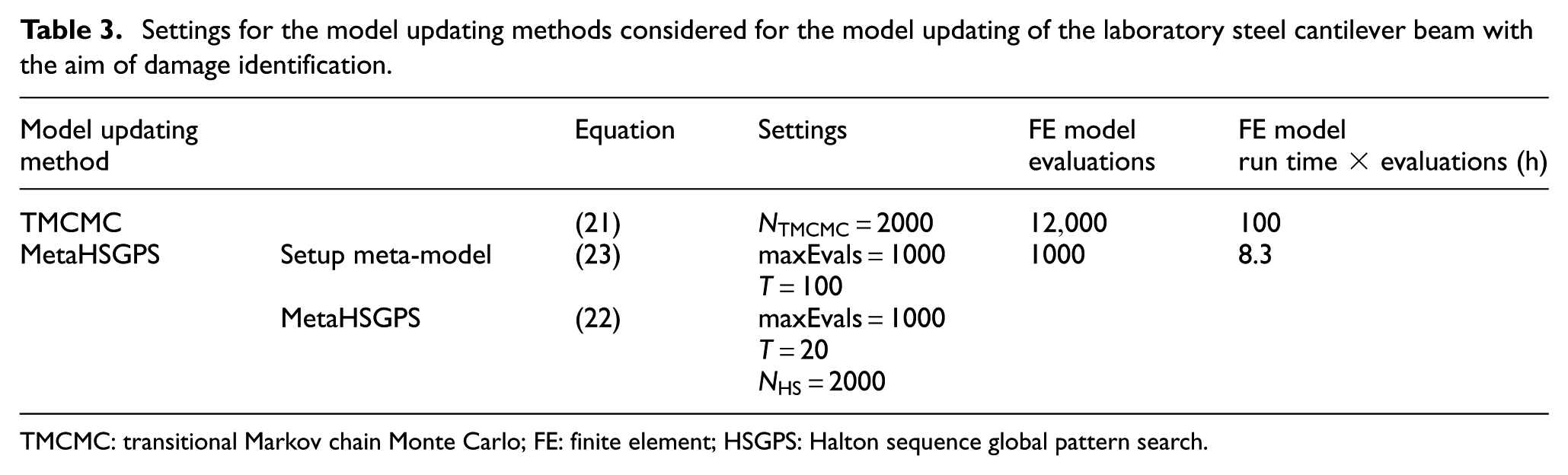
TMCMC: transitional Markov chain Monte Carlo; FE: finite element; HSGPS: Halton sequence global pattern search.
In the table, the number of FE model evaluations of the TMCMC algorithm is given as
In Figure 15, a comparison of the resulting CDFs of the TMCMC and metaHSGPS algorithms for all nine damaged fishplate positions is shown. The results are obtained using the settings listed in Table 3. A first overview of the results shows that the TMCMC and metaHSGPS algorithm generally provide similar results for the model updating of the steel cantilever beam with the aim of damage identification. However, it is noticeable that the results of the metaHSGPS algorithm show a clearer, more distinct convergence behavior.
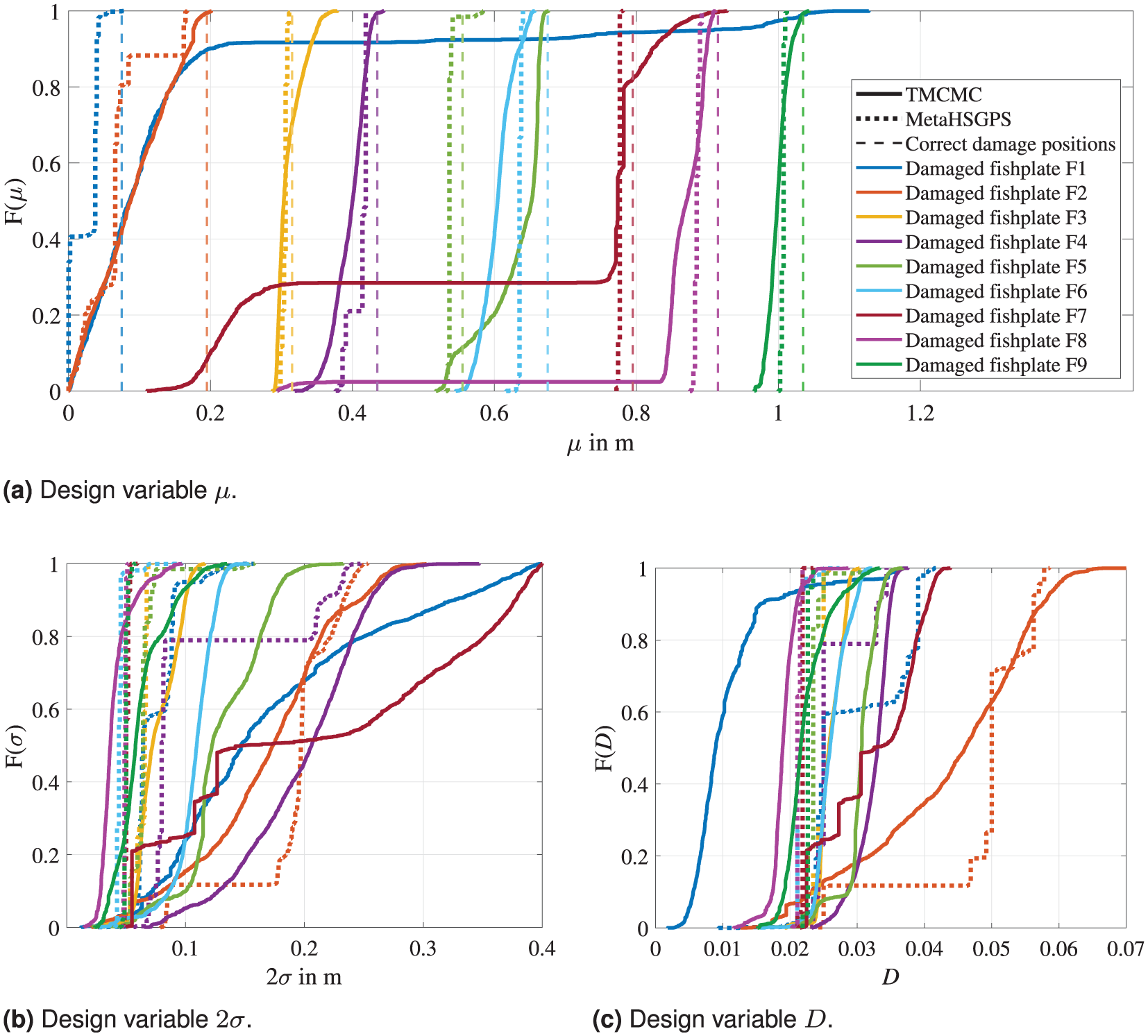
Comparison of the CDFs calculated by the TMCMC and metaHSGPS algorithms for the model updating of the laboratory steel cantilever beam using the fishplate with the uniformly distributed damage (cf. Figure 11). Results are shown separately for the three design variables, including all nine fishplate positions. The legend applies for all sub figures. (a) Design variable
The true values expected for the two design variables
Looking more closely at the localization results in Figure 14(a) (i.e., the results for design variable
To be fair, the TMCMC method may exhibit more variance in the results due to its inherent random basis (cf. Appendix section “A.1. Number of samples for the transitional Markov chain Monte Carlo algorithm”). If the TMCMC algorithm were to be run a few more times on the same model updating problem, the results might improve for some of the damaged fishplate positions, while some results might conversely deteriorate. As it is not the aim of this work to improve the scattering associated with the TMCMC method, but to present an alternative model updating procedure, the ability to choose an SDMU realization that provides deterministic, reproducible results is emphasized as a great advantage.
Conclusions and outlook
In this work, an alternative model updating procedure considering input uncertainty is introduced, which combines a sample provision with a numerical optimization algorithm. The general idea of the approach proposed is to exclude the uncertainty processing from the objective function formulation and, thus, from the actual model updating procedure. Instead, the uncertainty is incorporated implicitly by providing multiple discrete input samples and, subsequently, performing multiple deterministic model updating procedures based on each input sample. This way, the updating process becomes a repeatedly performed deterministic optimization problem, giving the proposed approach the name SDMU.
The main motivating factor for the proposal of the SDMU approach is its independence of previous assumptions about the input data (advantage No. 1 in the section “Introduction”). This is possible because the uncertainty incorporation is completely decoupled from the actual model updating procedure, which entails two key consequences: Firstly, the decoupled and resulting modular setup of the SDMU approach facilitates an arbitrary choice of the type of sample provision and optimization algorithm that make up a specific SDMU realization. This interchangeability makes the approach fully adaptable to the specific problem at hand (advantage No. 2 in the section “Introduction”), giving the user a lot of freedom for modifications and enhancements with regard to individual problem formulations. It also allows certain SDMU realizations to be selected in such a way that they deliver fully reproducible results (advantage No. 3 in the section “Introduction”). Secondly, any kind of stochastic input data can be propagated. The sample provision can either comprise the application of any type of sampling method—requiring assumptions about the input data—or may comprise simply taking experimentally gained data points as input samples—requiring no assumptions about the input data. Furthermore, a coupling to meta-models is easily facilitated, as the set-up procedure is inherently implemented within the SDMU approach (advantage No. 4 in the section “Introduction”).
These four main advantages of the SDMU approach are demonstrated in detail using a simple analytical 2DOF model updating problem and a laboratory steel cantilever beam, where the objective is structural damage identification. In all cases, the results of the selected and investigated SDMU realizations are compared to the results obtained using the TMCMC algorithm, chosen as a well-known and established benchmark BMU sampling method. Both applications confirm the validity of the SDMU approach proposed and demonstrate that the presented SDMU realizations show a clear and more distinct convergence behavior compared to the TMCMC algorithm. In addition, the findings clearly underline that the results of the respective BMU and SDMU methods directly reflect their input data. This, in turn, emphasizes the advantage of the SDMU approach to be independent of assumptions about the input data, but to be able to directly and, thus, correctly reproduce its characteristics.
As the computational cost for more complex numerical models becomes unfeasible without incorporating a meta-model in the SDMU approach, it should be noted that certain applications may require frequent retraining of the meta-model. For instance, environments with highly variable or unpredictable operating and environmental conditions can reduce the reliability of a meta-model.
An obvious and straightforward extension of the SDMU approach proposed is to extend the optimization to multi-objective. This way, in future studies, the uncertainty may be further reduced by incorporating additional information into the objective function formulation such as mode shape deviations.
Footnotes
Appendix
B. Experimental validation: laboratory steel cantilever beam
Declaration of conflicting interests
The authors declared no potential conflicts of interest with respect to the research, authorship, and/or publication of this article.
Funding
The authors disclosed receipt of the following financial support for the research, authorship, and/or publication of this article: We gratefully acknowledge the financial support of the Federal Ministry for Economic Affairs and Energy [research projects V|Pile—Influence of vibration parameters on the installation and the load-bearing behavior of monopiles, FKZ 03EE3022C, and MMRB-Repair-care—Multivariate damage monitoring of rotor blades: implementation and analysis of the effects of repair measures, FKZ 03EE2043C], which have made this work possible. In addition, we gratefully acknowledge the financial support of the German Research Foundation (Deutsche Forschungsgemeinschaft, DFG) [SFB-1463-434502799 and research project Effizienzsteiger-ung unscharfer Strukturanalysen von Windenergieanlagen im Zeitbereich (ENERGIZE), project number 436547100].