
Abstract
Corrosion under insulation (CUI) inspection is crucial for asset owners using insulated steel pipes susceptible to CUI, such as steam transport pipes. Current systems are effective for areas of corrosion above 0.01 m2 but are liable to miss small, deep localised corrosion below this size, which is the focus of the work presented. Defect sizing equations for a new encircling coil eddy current system have been developed from 2D simulation results. Tests of these equations on randomly sized defects in 2D simulations have shown an average error of 10%. In addition, 3D simulations confirmed that 2D results effectively translate to 3D, assuming a minimum circumferential extent. Initial lab tests of regular defects showed results comparable to simulations, but minor sensor placement errors can cause significant variations. This system’s potential to detect corrosion as short as 5 mm in the axial direction has been shown with a wall thickness error of 10%. However, this effectiveness is limited to specific corrosion and pipe morphologies; further study is required to expand these limits and to produce a system capable of detecting pitting corrosion in a wide range of applications.
Introduction
Background
Insulated steel pipes transport steam in various industries where process heat is used. Much of this insulated pipe is susceptible to corrosion under insulation (CUI), occurring when water penetrates the weatherproofing and condenses on the surface of the pipe. This moist environment causes corrosion to occur, as described in Wilds. 1
Conventional methods and limitations of existing approaches
In many facilities, the standard practice is to remove the insulation and visually inspect pipes to determine if corrosion is occurring. However, several non-destructive testing technologies, including X-ray, guided ultrasonic and eddy current systems, have been applied to this inspection problem in recent years. Each of these systems has advantages and disadvantages that are explored in Wilds, 1 Amer et al., 2 and Cao et al. 3 X-ray-based systems introduce the health and safety issues associated with a radioactive source. Still, they can produce good images of complex structures like valves and flanges that are not quickly inspected with other technologies. Ultrasonic inspection requires physical contact with the pipe, which requires breaking the weatherproofing. This issue can be reduced with a guided ultrasound system, which can inspect 50 m in optimal circumstances. However, any interruption in the pipe wall from joints, supports, bends and flanges requires additional holes in the weatherproofing. Available eddy current testing systems are pulse eddy current systems, which are highly portable and can accurately measure the remaining wall thickness if the corrosion appears over a large area. If the corrosion is highly localised, the magnetic footprint of these systems limits its ability to detect or accurately size corrosion. For example, the Eddyfi PECA-6Ch-MED tool has a minimum defect detection size between 120 and 49 mm, depending on defect depth, at 38 mm of lift-off. 4
The work presented in this paper is for an eddy current system that uses a continuous excitation signal, which will be referred to as a ‘continuous eddy current system’ to avoid confusion with pulsed eddy current systems commonly used in the CUI application space. The current system has been previously described in Bailey 5 and Bailey et al.6,7 This system shares the benefits of a pulsed eddy current system, requiring no break in the weatherproofing or special health and safety concerns. However, its spatial resolution is not limited by a magnetic footprint, as happens in the pulsed eddy current system. This means it can potentially detect highly localised corrosion that is not detectable with other systems. In previous work, the measurement method was developed, defect detection was achieved, and the effect of sensor alignment was explored.5–7
However, these previous works could not determine the extent of the corrosion, commonly reported as remaining wall thickness. This metric is essential to determine the remaining strength margin before a pipe rupture occurs. Previous work has not found a clear relationship between defect depth and a measurable magnetic field parameter. At best, a moderate correlation was found between peak radial field and defect volume, as shown in Figure 1. 6
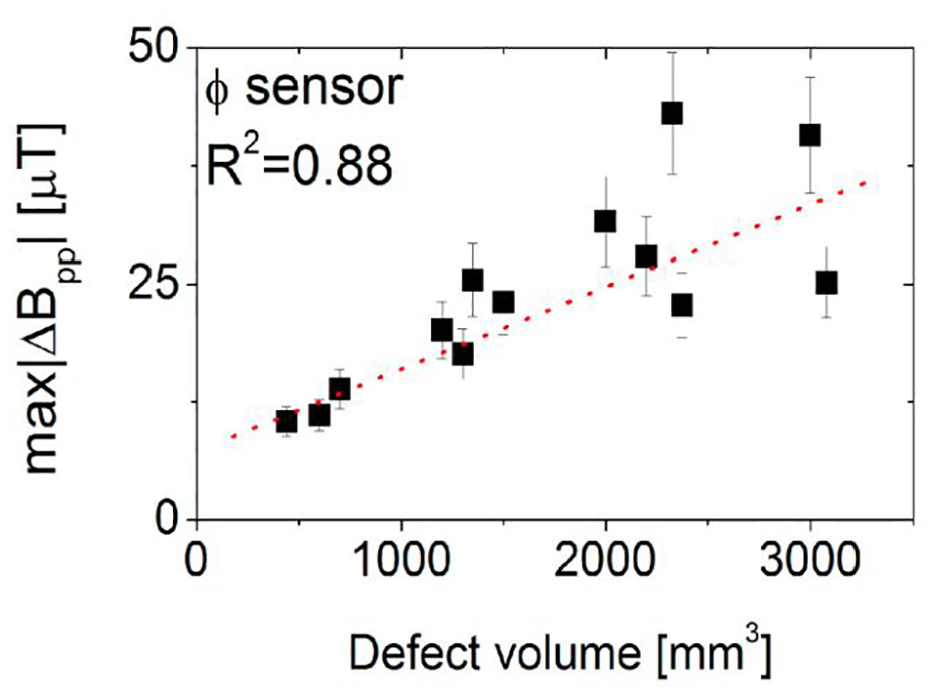
Relationship between volume loss and magnetic field distortion found in Bailey et al. 6 This indicates a moderate correlation but could not be used to accurately size defects.
A wide range of studies have explored the problem of sizing defects in steel with a continuous eddy current system, for example, Rifai et al., 8 Tsukada et al., 9 Yoshimura et al. 10 and Mohseni et al. 11 However, this sizing work has been done with defects in the order of millimetres and a coil-to-steel distance of no more than a few millimetres. This measurement geometry does not translate well to CUI defect inspection. Firstly, thick thermal insulation means the distance between the pipe surface and the measurement can typically range from 25 to 150 mm. Secondly, the shape of the defect is different; instead of thin cracks and pinholes being the concerning defect, defects with larger surfaces are the likely result of CUI. This can be observed in the many photographs of CUI, for example, in Javaherdashti. 12 The surface area covered by CUI can vary widely, from general area corrosion, which is several square metres in size, to localised pitting, with areas of 100 mm2 or smaller.
The use of a measurement system with an encircling coil and off-axis field measurement significantly changes the measurements, compared to typical eddy current systems where the coil axis is perpendicular to the surface of the test object, as used in Rifai et al., 8 Tsukada et al., 9 Yoshimura et al. 10 and Mohseni et al. 11 This means that sizing methods and systems developed for standard eddy current systems will not translate well to this novel measurement system, and new sizing methods need to be developed and verified.
Proposed method and contributions
This paper now explores the effect of defect size on the shape of the magnetic field in order to develop methods to determine the remaining wall thickness from magnetic field measurements. It initially models a simplified 2D system, showing how the depth of corrosion can be determined by measuring the radial magnetic field. This can be used to determine the critical remaining wall thickness for a known pipe thickness. These results will be confirmed in 3D simulations and selected experimental measurements.
The main contribution presented in this paper is the reporting of the effect of defect size on the measured magnetic field for an encircling coil eddy current testing system used on pipelines, as well as the proposal of defect sizing methods. This encircling coil eddy current system is proposed as an alternative to the pulsed eddy current system typically used in the inspection of pipelines through thick thermal insulation that has been discussed in many papers, such as Amer et al., 2 Cao et al. 3 and Eltai et al. 13 The potential advantage this system has over pulsed systems is the ability to detect and size small defects in pipes with thick thermal insulation. Pulsed eddy currents have a metric, referred to as their footprint, with defects below this size either undersized or potentially undetected. This is discussed in Xu et al., 14 which shows a reduction in probe footprint from 120 to 100 mm. The encircling eddy current system presented here does not have this footprint constraint, giving it the potential to detect and size much smaller defects.
An attempt has been made to size defects with this system in our previous work. 5 These results showed that no single parameter drives the amplitude of the magnetic field distortion, meaning that a method to determine the remaining wall loss, and thus, the remaining strength of the pipe, had not been achieved. 5 This paper aims to identify how different parameters affect the magnetic field and how the peak radial field and other metrics can be used to determine the remaining wall thickness.
Methodology
Two-dimensional simulation
To investigate the effect of defect size on the magnetic field measured by an encircling eddy current tool, a simplified axis-symmetric 2D simulation was developed in Opera™. 15 The simulation layout is illustrated in Figure 2. The simulation is axis-symmetric around the rotational axis of the pipe. This results in two simplifications. Firstly, no magnetic field is generated in the tangential direction as the eddy current is uniform in the circumferential direction. Secondly, the defect is uniform around the entire circumference of the pipe, which is not the typical shape of corrosion but reduces the parameters that affect the magnetic field, enabling effective simulation of the effect of the remaining defect parameters. The impact of a defect circumferential edge can then be assessed separately in a 3D simulation and will be demonstrated later in the paper.
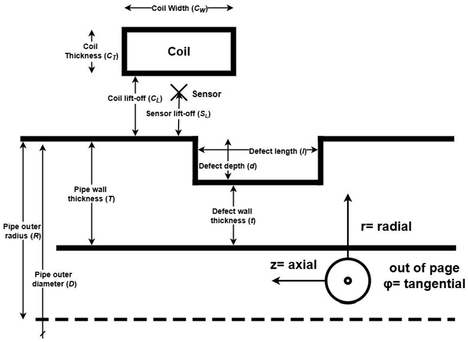
The layout of axis-symmetric 2D simulation of defective steel pipe with encircling excitation coil with coil travelling from right to left. Not to scale. Defect Depth will be referred to as (d), Defect axial length as (l), remaining wall thickness as (t) and pipe thickness (T).
When the pipe is uniform and the sensor is placed on the symmetry line, the eddy current on either side of it is also symmetrical. This results in the radial field contributions from currents on either side cancelling each other, resulting in zero radial field. This means when there is any asymmetry in the eddy current, caused by a change in geometry or steel properties, the radial components no longer cancel at the sensor location, and a radial field is observed. For the purposes of the simulation, the steel properties will be assumed to be uniform as these changes are small compared to the effect of corrosion.
When corrosion occurs, the steel is converted to a corrosion product comprising a mix of iron oxides and cavities, which can be considered a composite material composed of iron oxides and air. The steel has a relatively high electrical conductivity, compared to the corrosion product, and so for modelling purposes, corrosion is treated as non-conductive without introducing any significant errors. The reduction in permeability when steel is converted to corrosion is significant but poorly defined as the specific composition influences the value. The permeability of composite materials is discussed in Ollendorff 16 and Trompetter et al., 17 where an equation is presented to calculate the permeability of the material. Assuming that approximately spherical, high-permeability magnetic particles make up 10% to 50% of the composite, the composite’s effective permeability can be estimated to range between 1.5 and 4. A permeability in this range will affect the magnetic fields at low frequencies. However, to focus this work on the effect of the loss of the underlying steel, the corrosion product will be modelled with a permeability of 1, and the inclusion of the permeability variations due to the corrosion product will be left for future work. This simplification will result in cleaner, more distinct peaks in the presented results, as the potential variations in the magnetic field caused by the corrosion product have been removed. The significance of this simplification is highly dependent on the nature of the corrosion product that would be present in the real world. For cases where corrosion product is mostly non-magnetic oxides, or corrosion has flaked off or been washed away, this simplification would have little effect on the results. For the unlikely case of densely packed magnetite as the corrosion product, the results from this paper would need to be reconsidered.
This means an area of corrosion can be considered a section of pipe with a thinner wall surrounded by transition areas where the wall reduces from the original wall thickness to a remaining wall thickness. If the location of each of these transition zones of wall thickness reduction, called edges, can be identified, then the extent of the corrosion area can be determined. Similarly, if the change in wall thickness at each edge can be determined, the remaining wall thickness in the corroded area can be determined.
To investigate how to identify these corrosion edges and determine their depth, a range of simulations have been completed with increasing complexity. This allows an edge detection system to be developed and assessed for accuracy.
Parametric study: effect of corrosion depth
The initial simulation has been further simplified to focus on just one edge of the defect with Figure 3 showing how the defect representation has been simplified from Figure 2. There are two ways to represent an edge, shown in Figure 3; (i) a simple single-step and (ii) the more representative chamfered edges.
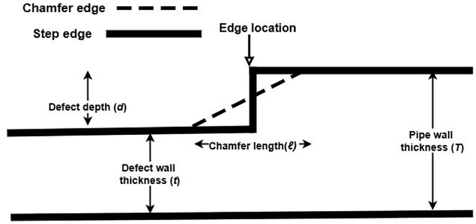
Different potential approximations of corrosion edge as used in simulations of pipe corrosion.
The first set of simulations uses a single-step edge. Dimensions are chosen consistent with our previous work and common pipe geometries. The original pipe wall thickness is T = 10 mm, and the defect depth is adjusted from d = 0.5–9 mm. A 50 mm wide, 5 mm thick coil is used with 50 mm coil lift-off and 40 mm sensor lift-off. The excitation field is generated by a 10 Hz 180 A current in the coil. For each simulation, the coil and sensor are moved 500 mm on either side of the single-step edge. Figure 4 shows the magnitude of the resulting radial magnetic field from these simulations. For defect depths <6 mm, the radial magnetic field consistently exhibits two distinct peaks, with the larger peak appearing on the side of the defect edge corresponding to the intact wall region. As the defect depth increases beyond 6 mm, this two-peak pattern transitions into a single dominant peak.
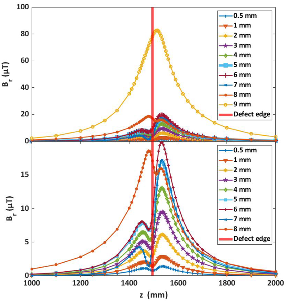
Effect of defect edge depth (d) on the radial magnetic field Br as a function of axial position z, for a pipe with an initial wall thickness of 10 mm. The top plot includes the dataset for d = 9 mm. In the bottom plot, this dataset is excluded to improve visibility of the remaining curves.
The relationship between the defect depth and size of the peak magnetic field is plotted in Figure 5. With the addition of 20, 40 and 10 Hz cases with a 15 mm pipe wall, this shows a linear relationship for the peak radial field with edge depth up to a frequency-dependent threshold. We define the linear slope as m = Br0/d. In addition, the change in threshold with pipe wall thickness shows that the value that determines this threshold is the defect wall thickness (t), not the defect depth (d). A defect wall thickness of 4 mm represents the turning point in both 10 Hz cases.
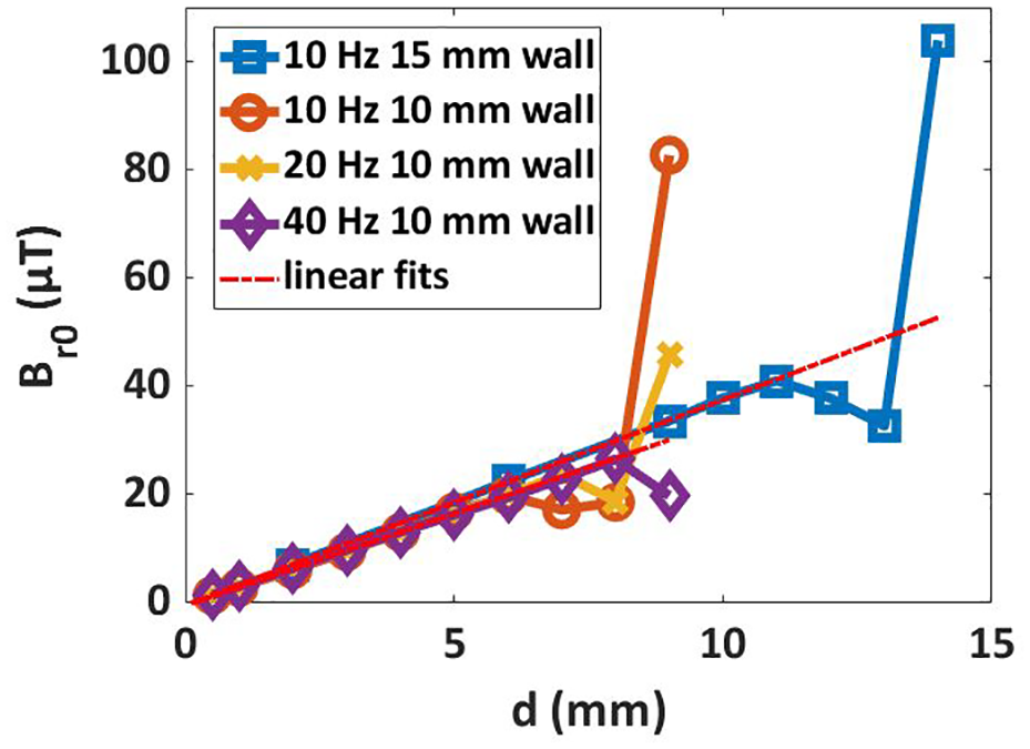
Peak Br (Br0) with defect depth for a range of excitation current frequencies at 10 mm wall thickness and one example of 15 mm wall thickness. Linear fits show that the extent of the linear zone with defect depth increases with increasing frequency and increasing wall thickness.
The turning point dependence on the frequency and defect wall thickness suggests that the defect wall thickness-to-skin-depth-ratio (δ r = (t/δ)) is the likely determining factor of the turning point. To confirm this, Figure 5 was replotted as a peak radial field against the ratio δ r in Figure 6, with δ calculated using values of 600 for the relative permeability from the Opera database 15 and a steel conductivity of 5,882,000 S/m. 18 This shows, as hypothesised, that a turning point occurs when δ r ≈ 1.5.
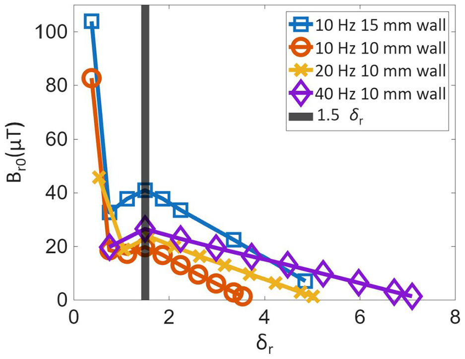
Effect of the remaining thickness-to-skin-depth ratio on the radial magnetic field for a range of frequencies and 10 and 15 mm wall thickness pipes.
This threshold, which will be represented by δ 0 , can be defined as the δ r that results in the maximum Br for values of δ r > 1. To understand why a threshold is reached at 1.5 δ, we must consider how the δ affects the eddy current density with depth and the effect of the inside wall boundary of the pipe. When the defect wall thickness is much greater than the skin depth, the eddy currents can be distributed with the standard 1/e decay. However, this distribution assumes that there is no inside wall boundary. This assumption becomes less valid as the wall thickness approaches δ.
Figure 6 does not have enough data points to resolve the transition from linear to non-linear dependence. To produce higher-resolution data of this transition, a frequency sweep of the excitation current from 0.1 to 10 Hz was simulated with defect depths of d = 2, 3 and 4 mm and T = 10 mm. The results are plotted in Figure 7, showing a smooth transition from linear to non-linear with δ0 shifting by 0.1 per millimetre of additional defect depth. In addition, this greater resolution shows δ0 ≅ 1.7.
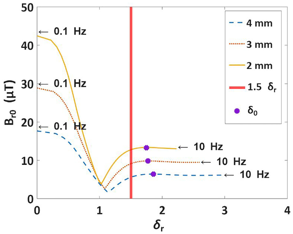
Simulation results with a frequency sweep from 0.1 to 10 Hz, with defect depths from 2 to 4 mm showing peak radial field versus remaining wall thickness in units of skin depths, at each frequency.
The result of the simulations in this section is that there are two potential methods to determine the defect depth when the defect wall thickness t > 1.7 δ. One measures the peak radial field (Br0) at a fixed frequency, and the other measures the frequency of the peak radial field. If the peak radial field (Br0) is measured, then the slope (m) from the linear fits found in Figure 5 can be used to determine the defect depth (d) using Equation (1).
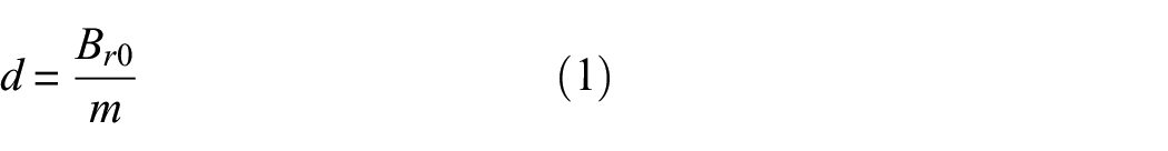
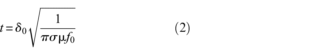
Alternatively, the defect wall thickness (t) can be determined using Equation (2). A frequency sweep is used to find the value (f0) in Equation (2), the frequency that produces max Br when δ r > 1. Figure 7 gives a value of 1.7 for δ 0 . σ is the steel’s conductivity, and µ is the steel’s permeability.
Determining the defect depth with Br0 measurement produces a more accurate depth measurement, but it needs an accurate magnetic measurement of a small defect signal that could be affected by a range of unaccounted-for effects, such as the sensor’s sensitivity value. Determining the defect depth with f0 measurement will be unaffected by these magnitude changes, which could make for a more robust measurement. However, as δ0 changes at a rate of 0.1 per mm of d, as seen in Figure 7, this will result in a systematic error that, if not addressed, will introduce an approximate error of 0.4 mm/mm for the defect depth. This was determined by substituting Δδ0 = 0.1 into Equation (2) with µ and σ values used in the simulations and the peak frequency found in Figure 7. This results in a maximum error of 2 mm for a 10 mm pipe wall thickness.
Two methods have been introduced that are independently capable of determining the edge depth, one using measurement of Br0, which will be labelled the peak radial field method, and the other using measurement of f0, which will be labelled the peak frequency method. Each method has different advantages and drawbacks.
The main advantage of the peak radial field measurement is its linear relationship, which means that the accuracy achieved in the peak radial field measurement is directly translated into accuracy in the depth measurement. However, magnetic fields drop rapidly with increasing distance between sensor and pipe. This causes the signal-to-noise ratio to drop for systems where the sensor is placed a long way from the pipe, for example, testing a pipe with 100 mm thermal insulation. Countermeasures to increase the signal-to-noise would introduce disadvantages such as requiring more time to scan or requiring larger drive currents in the source coil.
The peak frequency method is a comparative method, so it requires precision in the magnetic field measurements but not accuracy. The disadvantage is the high expected error in the defect depth, with up to 2 mm expected in a 10 mm pipe wall thickness.
In an ideal implementation, both peak frequency and field measurements would be used on the same tool, with further investigations to determine how these can be combined for the most accurate result.
Parametric study: effect of corrosion boundary shape
Having achieved a good defect depth equation, with the limitations laid out in the previous section, the effects of changing the stepped edge to a chamfer edge were now considered. Figure 3 shows a more realistic approximation of corrosion in a real pipe, as a gradual change in wall thickness from nominal to defect wall thickness would be expected.
An extra parameter is needed to define a chamfered edge. In addition to the defect depth (d), a chamfer axial length (ℓ) is needed to define the edge fully. Simulations were completed at various defect depths and chamfer axial lengths, with the results shown in Figure 8.
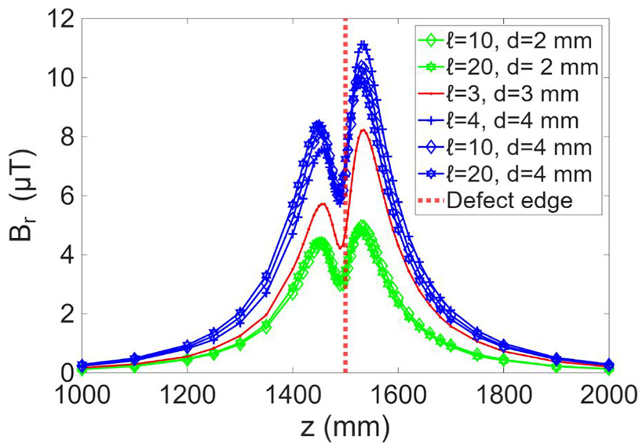
Effect of changing chamfer axial length (ℓ) and defect depth (d) on the radial magnetic field.
These results showed that the predominant factor was the depth of the defect, with increasing chamfer axial length only producing a slight peak value reduction and broadening of the peak. Specifically, Figure 8 shows a change of 1.2 µT for a chamfer axial length change from 4 to 20 mm (with d = 4). When using the peak radial field calculation from the previous section, this results in a depth error of 0.5 mm. This shows that approximating the chamfered edge as a single step is a valid approximation with minimal loss in accuracy.
The alternative method to determine edge depth uses the peak frequency. To test the effect of a chamfered edge on peak frequency, a simulation of a 4 mm deep defect with a 4 mm long chamfer was compared with a 4 mm deep stepped edge, as shown in Figure 9.
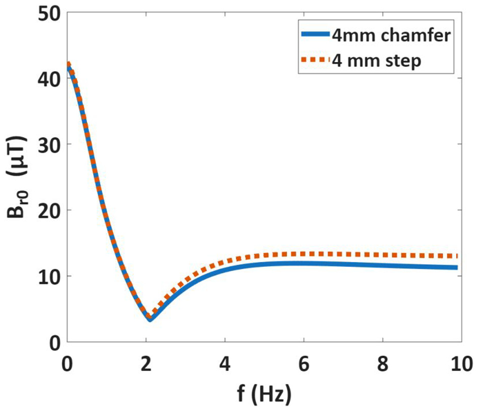
Comparison of peak radial field Br0 with excitation frequency for a single-step edge and a chamfered edge.
In Figure 9, it can be seen that the presence of a chamfered edge only leads to a shift of 0.4 Hz in the peak frequency. This would result in a 4% depth error for a 5 mm defect depth. This means that the shape of the edge has a minimal effect on the peak frequency method of determining defect depth, and that both edge depth calculation methods can be approximated as stepped edges for the purposes of simulation. For the remainder of the paper, a stepped edge will be used to approximate defect edges.
Parametric study: effect of corrosion axial extent
Until this point, the simulation has focused on the effect of a single edge. However, a defect in a 2D space needs two edges to create an area with a thinner wall compared to the surrounding wall thickness. The defect can be defined with two parameters, the defect depth (d) and defect axial length (l), as shown in Figure 2.
A set of defects has been simulated with a range of defect axial length values from 5 to 1000 mm and a fixed d = 4 mm, with the results shown in Figure 10. The results from the simulation show that, above a defect axial length threshold of 200 mm, the magnetic field produced by a defect edge is not affected by the other edge that makes up the defect. This 200 mm threshold has been determined by data in Figure 10 by observing the peaks located at the z = 35 mm location where they are stacked on top of each other. The 1000, 400 and 200 mm peaks all appear to lie on top of each other, with the first significant change observed for the 100 mm long defect. Conversely, for defect axial lengths below this threshold, the location of the second edge affects the magnitude of the peaks.
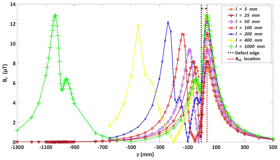
Radial magnetic field over 4 mm deep defect with varying defect axial length, l, simulated and calculated results with 10 Hz excitation. The defect edges are at z = 0, and z = −l.
The simulations have shown that two values can easily be extracted from the measured radial magnetic field: the peak magnetic field (Br0) and the spacing between the peaks (ΔzB). These two values can then be used to calculate the defect axial length (l) and the defect depth (d).
To calculate defect axial length, we introduce a new variable εz, which is the z distance between defect edge and the peak radial field that it produces. This value is shown in Figure 10, where it can be observed that all peaks from the fixed defect edge location at z = 0 mm are 35 mm from the defect edge. This empirically determined value can be used with ΔzB in Equation (3) to calculate defect axial length (l).

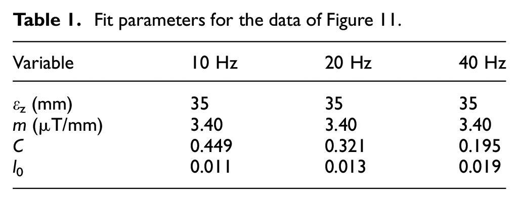
The defect depth calculation is split into two cases depending on whether ΔzB larger or smaller than a threshold, in this case 270 mm. From Figure 10, this transition value can be empirically determined to be approximately l = 200 mm. Adding the 2εz gives a ΔzB threshold of 270 mm. For the case ΔzB > 270 mm. Equation (1) can be used to determine defect depth (d) with the empirically determined slope (m) values reported in Table 1.
Fit parameters for the data of Figure 11.
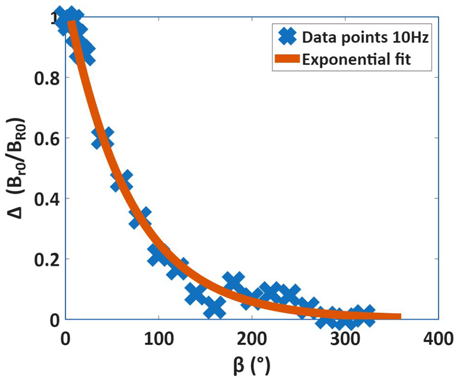
For the case ΔzB < 270 mm, we require a different method. We observe from the simulation results in Figure 10 that as the edges of the defect get closer together, the peak radial field generated for a given defect depth is reduced. The fractional loss in amplitude Δ
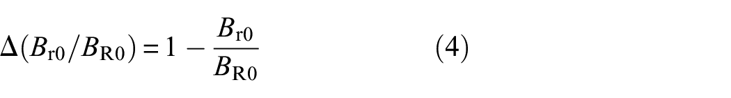
where
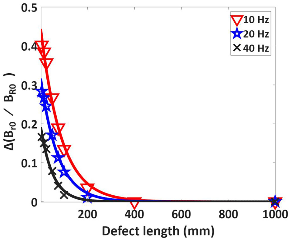
Defect axial length effect on the change of peak radial magnetic field for the results of Figure 10.
For each frequency, we can fit an exponential curve represented by Equation (5) to calculate the fractional loss Δ

Combining Equations (1), (3), (4), and (5) and the Br value from the simulations, we can calculate defect depth (d) for any defect size as:
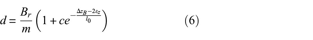
This equation has been derived using results for a ‘typical’ defect of depth d = 4 mm in a T = 10 mm total wall thickness pipe. In the next section, we test whether this method is robust against changes in defect dimensions.
Summary of accuracy assessment
To test the effectiveness of the defect sizing using Equations (1) and (6), a set of randomly sized 2D defects was simulated using the model as shown in Figure 2. The parameters used are broadly the same as in the previous simulations. A 50 mm wide, 5 mm thick coil is used with 50 mm coil lift-off and 40 mm sensor lift-off. The excitation field is generated by a 10 Hz 180 A current in the coil. For the steel, a relative permeability value of 600, and a conductivity of 5,882,000 S/m was used. With the values for d, l and T generated by a random number within a min–max envelope, the values simulated are recorded in the first three columns of Table 2. A minimum remaining wall thickness of 4 mm was used to ensure the response was in the linear region, as shown in Figure 5. With the 10 Hz excitation, this means t > 4 mm. The resulting Br0 and ΔzB values were extracted from the simulation outputs, and the values of d and l were calculated. A summary of these results is shown in Table 2. Good results were achieved with the error in d as a percentage of T <10% for all except one. This outlier has a pipe thickness that is significantly larger than the value used in the simulations that developed these equations, suggesting that a more detailed analysis should account for increasing pipe thickness for a fixed frequency.
Defect sizing testing results.
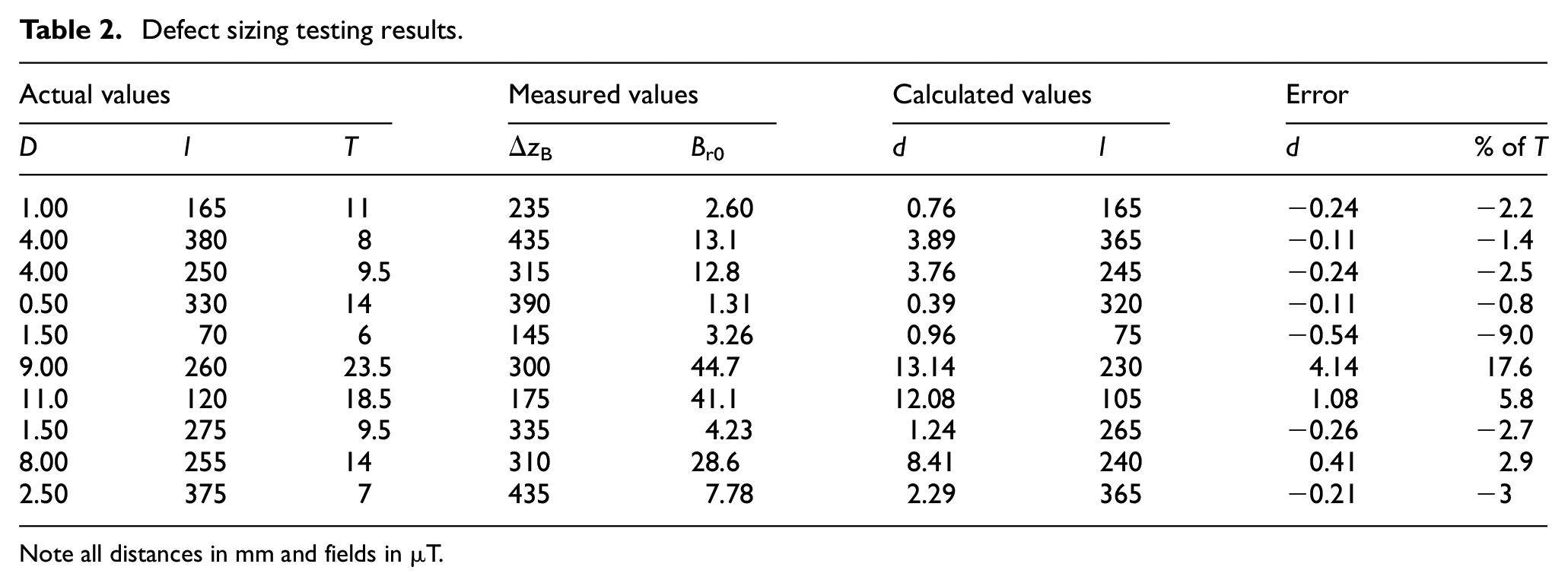
Note all distances in mm and fields in µT.
Plotting the error in calculated defect depth as a percentage of pipe thickness from Table 2, with respect to pipe thickness in Figure 12, shows that a larger error is produced when the pipe wall thickness deviates too much from the 10 mm thickness on which the equation was developed. In practice, the equations used would be tailored to the geometry of the pipes under test.
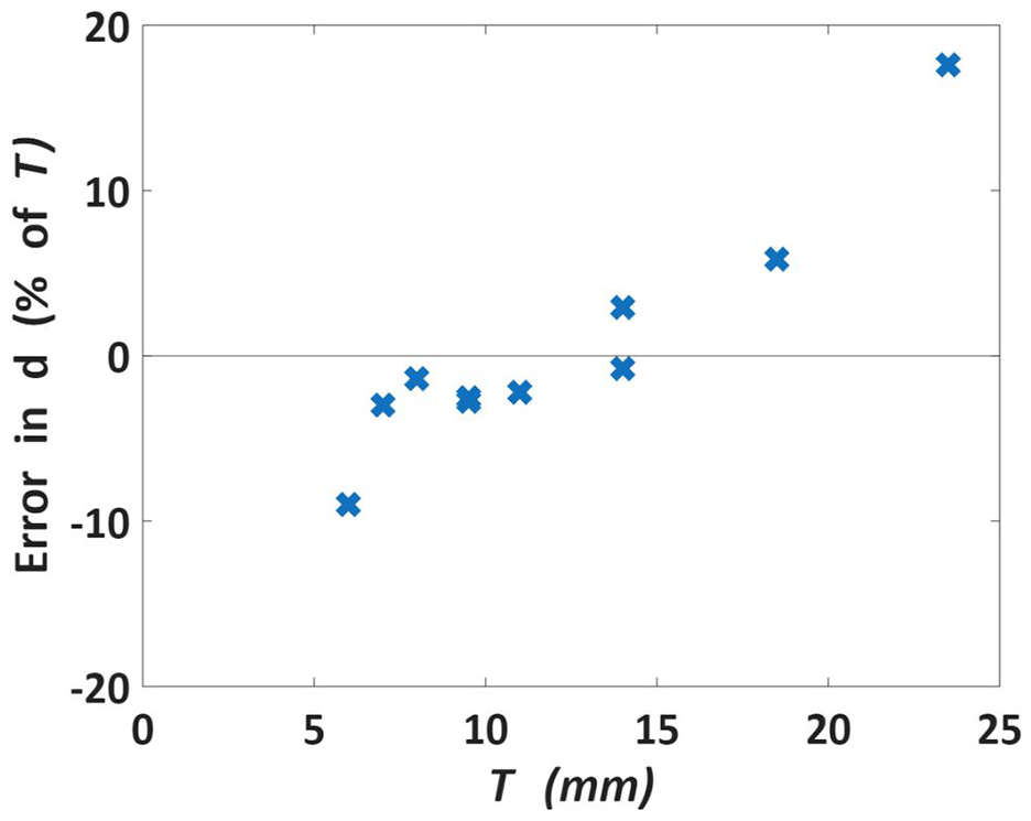
Remaining error in defect depth calculation with respect to the pipe wall thickness.
Three-dimensional simulations
Up to this point, the simulations have only considered a rotationally uniform pipe, which means that all the defects simulated have two edges, which are referred to as z edges. However, in real applications, defects are likely not to extend around the whole circumference of the pipe, meaning an additional two edges are introduced, referred to as φ edges. A deep exploration and extension of the sizing equations to three dimensions are beyond the scope of this paper. However, an initial analysis of how the 2D results compare to the 3D results is presented in this section.
One of the previous 2D simulations has been repeated in 3D to ensure consistency and to validate the 2D simulations used up to this point. This was completed for one pipe model with a 4 mm deep, 200 mm long defect. The 3D simulation was completed for five z positions starting from one edge of the defect, where a peak in the field is produced. The 2D and 3D simulation results are compared in Figure 13 and show good agreement with an average radial magnetic field error of 1.4%. This confirms the consistency between the 2D and 3D simulations in this paper.
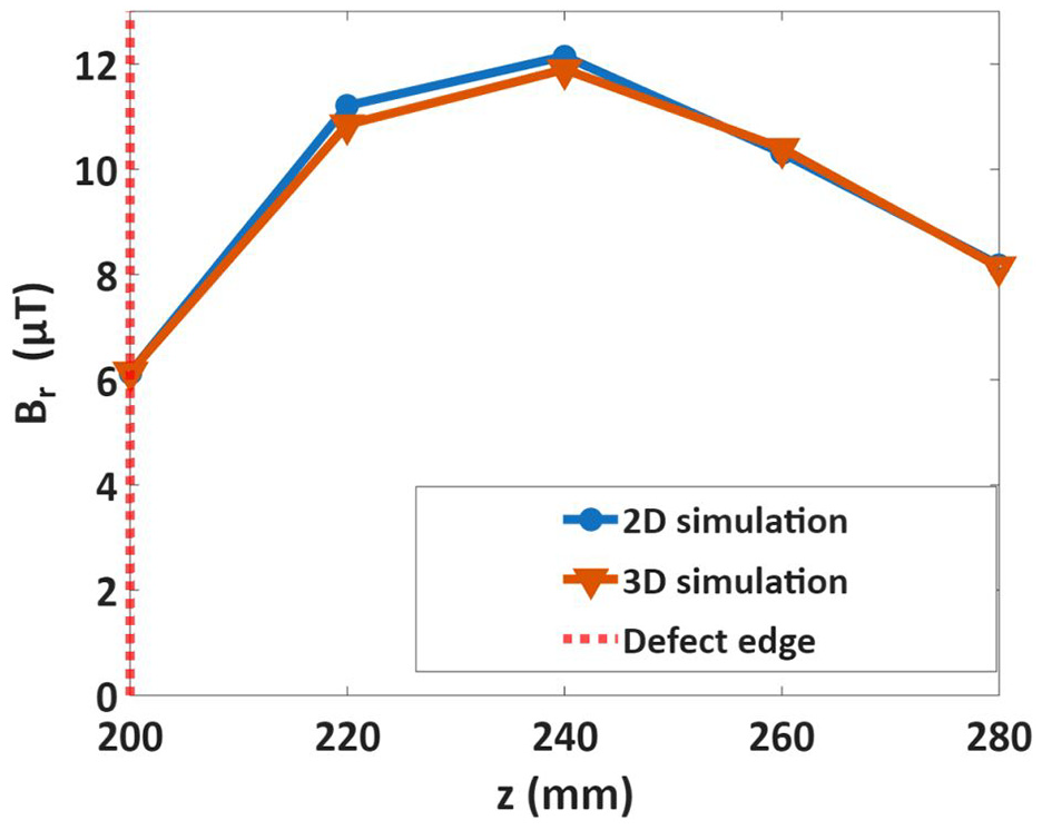
Comparison of 2D and 3D simulations of a pipe with a 4 mm deep defect 200 mm long that extends the whole circumference of the pipe.
Parametric study: effect of corrosion circumferential extent
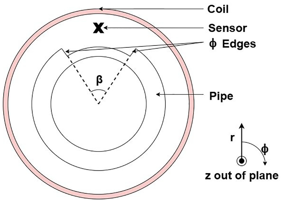
The φ edges are defined by the angle β shown in Figure 14. To simulate a sweep of β values, an assumption is made that the z position of the peak radial field would be static with the offset εz = 35 mm, as reported in Table 1. This assumption was made because changing the axial length of the defect (l) had no effect on εz.
β Angle defines the location of the defect φ edges.
Using this assumption, a 4 mm deep, 400 mm long defect was simulated with the coil and sensor located 35 mm outside the z edge, the location of the peak radial field in the 2D simulations. The β angle for the defect edges was then swept from 350° to 1°. As seen in Figure 11, the fractional loss of the nominal field has been calculated and plotted in Figure 15.
Effect of φ edge angle on Br 35 mm from z edge.
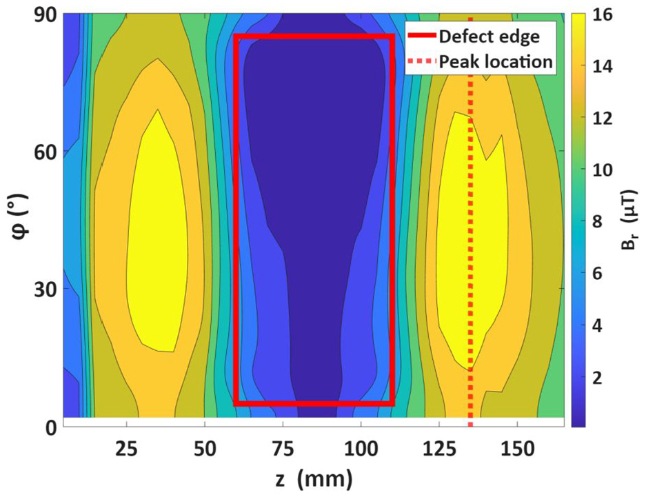
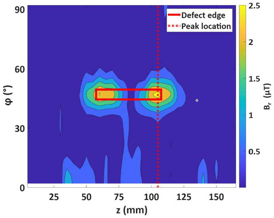
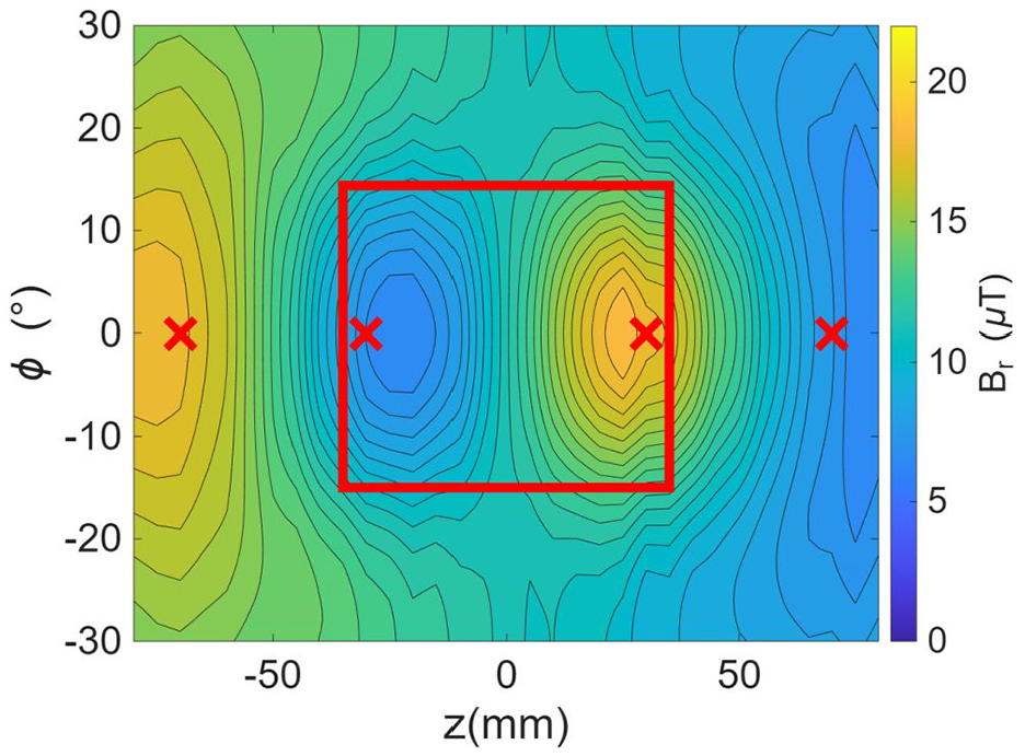
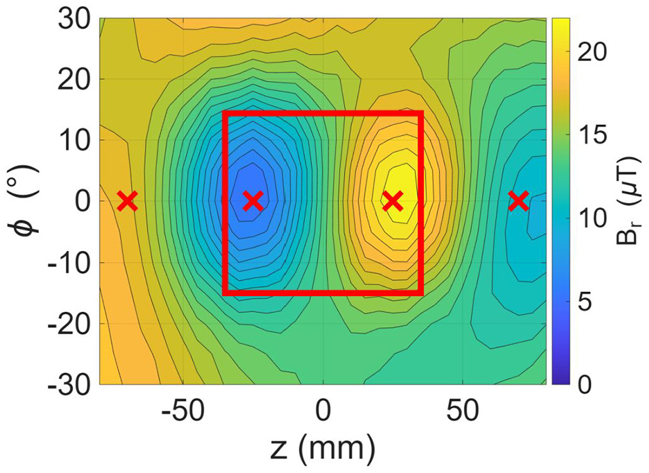
The φ edge spacing appears to produce an exponential decay in the peak radial field, much like the z edge spacing. However, a full simulation of defects that are 50 mm long with β angles of 80° and 5° reveals that the assumption of static peak location with a εz = 35 mm does not hold for all β angles. For the 80° case shown in Figure 16, there is a slight shift in peak location to a εz = 25 mm. For the 5° case, shown in Figure 17, there is a large shift in the peak shift with εz = –5 mm.
Contour map of radial magnetic field over a 4 mm deep, 50 mm by 80° defect.
Contour map of radial magnetic field over a 4 mm deep, 50 mm by 5° defect, showing the peak location shifted to inside the z edges.
We theorise that the cause of this shift in peak location is due to finite values of β producing eddy currents that do not strictly flow in the circumferential direction, which is illustrated in Figure 18. Instead, at each corner of the defect, the eddy current will bend around the end and redistribute itself evenly along the φ edge of the defect. For the small β case, this effectively produces a circulating current at the z edges of the defect. This circulating current will produce a radial field inside the z edge of the defect, as seen in the simulation results in Figure 17. In the large β case, the corners where the eddy current is bent are spaced further apart, so it is expected that the radial field produced by non-circumferential eddy current will make only minor changes from the infinite β case.
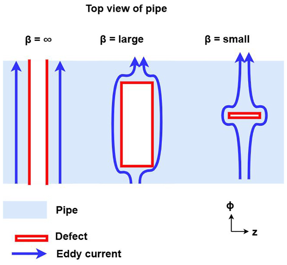
Effect of β angle on eddy current flow in pipe.
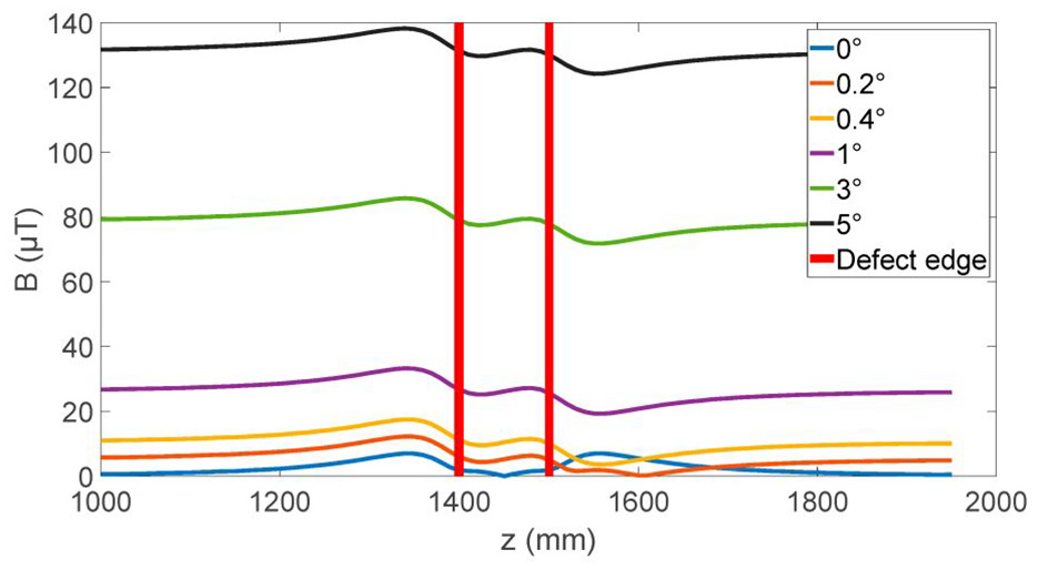
Given the shifting peak location that appears to be dependent on β, the question that will guide further exploration is: at approximately what value of β do the peaks transition from outside the defect, approximating an infinite β response, to inside the defect edges, resulting in the small β response? To answer this, a set of 3D simulations for a range of β values was completed, with the resulting Br values plotted in Figure 19. The magnetic field has been normalised to a peak of 1 for each β to eliminate magnitude change, allowing for good visualisation of the peak value location. The plots in Figure 19 show that the transition occurs at approximately β = 20° where the peak inside the edge is approximately equal in amplitude to the peak outside the edge. However, this is a relatively slow transition, with inside peaks appearing in the 40° case, and the outside peaks remain present in the 10° case.
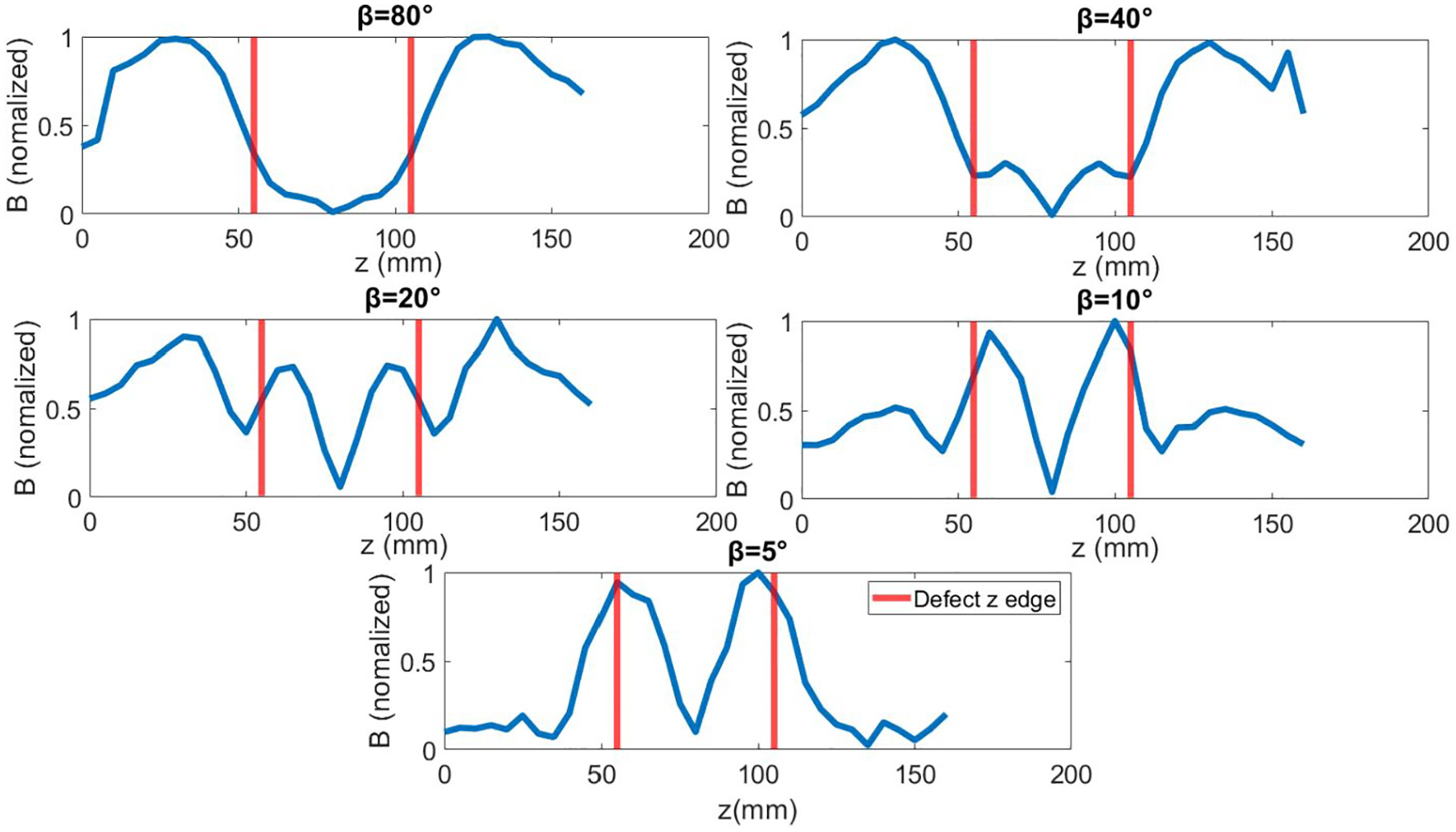
Peak radial magnetic field location shifts from outside of edge to inside of edge with a decreased φ edge β angle. Magnetic fields have been normalised to 1 for each case.
The underlying mechanism for this transition and how to size defects that have crossed this threshold is outside the scope of the work presented here. However, we can say that for defects such as those where the peaks occur outside the z edges, for example, a defect with a β angle larger than 20°, the sizing equations developed should still be effective because up to this threshold, the peak pattern follows that of the 2D simulations. Extending our defect sizing models to be valid for smaller defects would require an expanded set of simulations to determine the peak radial field behaviour with defect depth, defect axial length and the β angle.
Experimental validation
A lab testing setup, as shown in Figure 20, was built to determine the accuracy of the simulations and to identify the additional limitations of this defect detection system. It consists of a rotation stage that rotates the pipe under inspection and a linear stage that moves the coil and magnetic sensor down the axial length of the pipe. This mechanical setup allows the whole surface of the pipe to be inspected (Figure 20).
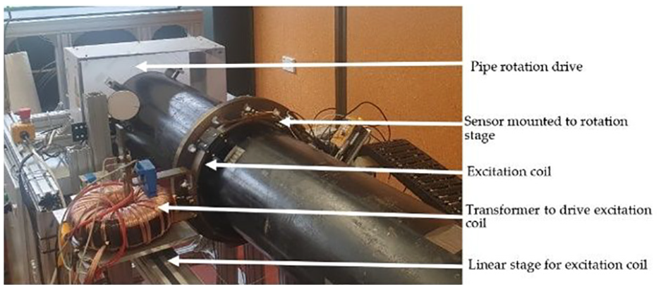
Lab setup for testing corrosion detection of steel pipes with an encircling excitation coil.
The magnetic field measurement is completed with a tunnelling magneto resistance (TMR) sensor produced by MultiDimension Technology, part number TMR2001 with a sensitivity of 0.08 mV/V/µT 19 resulting in a sensitivity of 0.4 mV/µT when powered by 5 volts. The TMR output signal is fed into a Stanford Research Systems SR830 lock-in amplifier 20 that uses the excitation signal as the reference. This setup achieves a background noise level of 0.022 µT.
The excitation current to the coil is sourced from a Hewlett-Packard 33120A signal generator, 21 which drives a high-power audio amplifier. The amplifier is an off-the-shelf bass amplifier from Zeroflex, model number NZ2000D, providing 2 kW @ 1 ohm. 22 This amplifier, in turn, drives a hand-wound toroidal transformer with a 60 × 60 mm core and 100 turns on the primary, with a single copper loop acting as the secondary winding. This setup allows for high currents with relatively low power. A current of 300 A has been used for the experiments presented here.
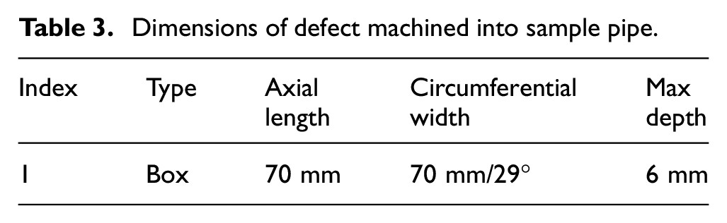
The defect simulated previously in this paper had a uniform depth to reduce the parameter space. However, defects in this shape are more complex and expensive to machine. In the experimental setup, a box defect was machined into the pipe, as shown in Figure 21. A total of eight different defects were machined in a 3 m, 10-inch steel pipe for testing. While all the defects were measured and simulated, we will focus on one for brevity, with its dimensions summarised in Table 3.
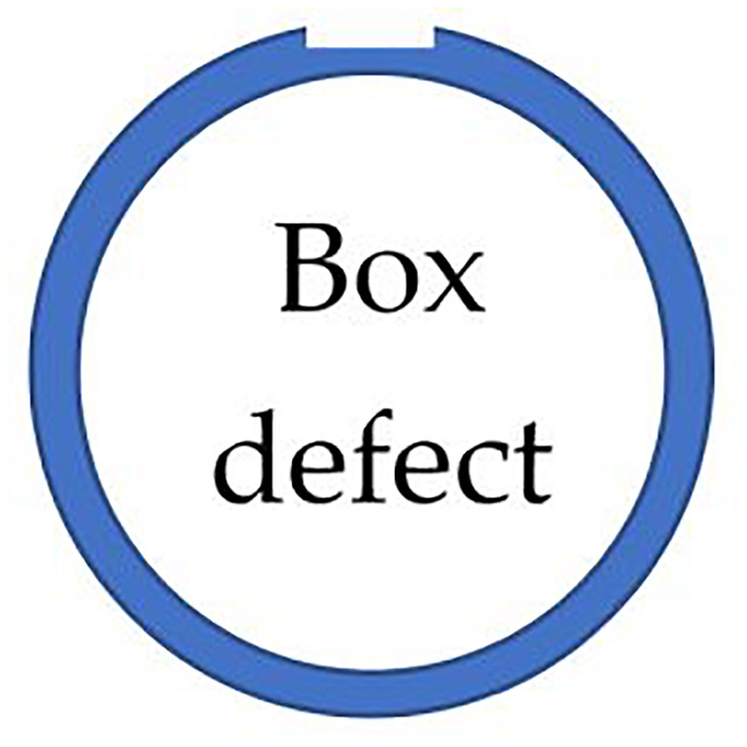
Shape of defects machined into sample pipe.
Dimensions of defect machined into sample pipe.
A 3D simulation of each machined defect was completed using the same process as in the 3D simulations section. The simulation parameters are summarised in Table 4. These parameters differ from previous values to match the experiment setup more accurately.
Simulation parameters for the simulation of lab testing.
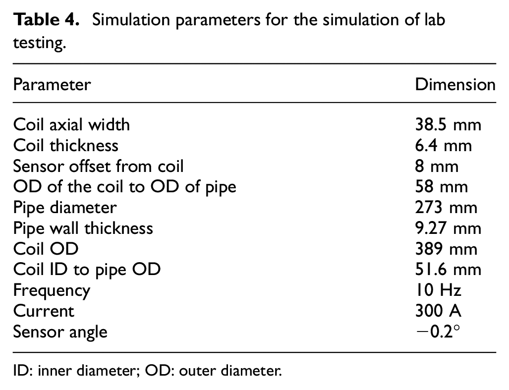
ID: inner diameter; OD: outer diameter.
A new parameter has been introduced called sensor angle, which is a measure of the misalignment of the sensor from being perfectly aligned with the radial direction. It is known from previous work in Bailey et al. 7 that this system is susceptible to this misalignment. The main result is that sub-degree changes in alignment will produce a large offset field and change the shape of the magnetic field from having two peaks to a local maximum and a local minimum, summarised in Figure 22 from Bailey et al. 7 This result allows an estimate of the sensor angle to be made by measuring the average background field in a defect-free location, then adjusting the sensor angle in the simulation to match a defect-free pipe to get the same field. In this case, this occurred with a sensor angle of −0.2°.
Effect of sensor angle on radial magnetic field when moved over a 100 mm corrosion defect. 7
It should also be noted that defect 1 has an angle β = 29°. Referring to the simulation of the effect of β angle in Figure 19, 29° is in the range where the peaks are shifting from inside the z edge to outside the z edge. This means a set of four peaks are expected. However, with a sensor rotation, this will instead be two local minima and two local maxima.
The results of simulating defect 1 are shown in Figure 23, showing a clear local maximum and minimum inside the defect edges and a second pair of local maximum and minimum approximately 40 mm outside the defect edges.
The simulated radial magnetic field over defect 1 with the sensor rotated 0.2°.
The experimental setup was then used to measure the magnetic field over the sample pipe. The measured radial magnetic field over defect 1 is plotted in Figure 24. When comparing Figure 24 to Figure 23, the most significant divergence is the distortion of the peak that appears at z = −75 mm in the simulation. However, the clear presence of the other maxima and the two local minima in the same locations gives confidence in the effectiveness of the simulations and their results.
Measured radial magnetic field over defect 1 with a red box showing the outline of the defect and red markers showing the expected peak locations to match the simulation.
The maximum circumferential width of the experimental defects was 29°. This means the 2D depth sizing algorithms cannot be tested for determining the depth of this experimental result, as from the 3D simulation, it was discovered that defects with a circumferential width larger than 80° are needed to use the 2D defect sizing algorithms without modification. What we have shown is that we can accurately simulate the generated magnetic field in the presence of defects using the full 3D geometry. To size defects when β < 80° will require developing an algorithm to accurately determine the β angle and then correct for the change in magnitude of the radial field.
Discussion
This study has used simulations to investigate the use of an encircling excitation coil eddy current system to identify and size CUI. This has been achieved with the caveats that the defect must be large in the circumferential direction and the sensor must be accurately aligned. With these limitations, defect depth can be determined with accuracy better than 1 mm until the remaining wall thickness reaches a threshold of between 4 and 2 mm, depending on the excitation frequency. The methods developed in this paper have been based around a nominal 10 mm thick pipe wall with deviation from this nominal wall thickness introducing increasing error in defect sizing. However, this error appears to be systematic in nature with roughly linear change in error with changing wall thickness. This relationship could be used in future work to provide pipe thickness error correction.
The 2D simulations showed that the effect on the radial magnetic field is dominated by the defect edge depth. In the case of a large defect axial length, there is a sufficient distance between the edges so that the corresponding edge does not have to be accounted for when predicting the radial field, and a simple linear relationship is found between the peak radial field and edge depth. This allows for accurate defect size identification for large defects. However, when the defect size is below a threshold value, an additional set of correction factors has been identified that can be used to correct for the effect that nearby edges have on the peak radial field, enabling correct defect sizing for these smaller defects. These simulated results show that a defect depth error of <1 mm can be achieved.
The 3D simulations have shown that the spacing between the φ edges affects the peak radial field location. A large β angle results in peaks outside the z edge. This means the defect sizing equations developed with the 2D simulations remain effective. Below a β angle threshold, the peaks shift to inside the z edge and magnitudes change, requiring new sizing equations to be developed for this case. Initial laboratory experiments of this encircling coil geometry have matched the simulation results when the effect of sensor rotation has been factored in. This shows that simulation results are valid and can be used to develop defect-sizing equations. The laboratory results highlight the sensitivity to sensor angle and the need to control this parameter accurately to achieve accurate defect sizing with this approach. Addressing this sensitivity to sensor alignment could be approached in a number of ways in future work: (i) A mechanical design could be implemented that allows for fine adjustment of the sensor angle via a set screw allowing correction of the assembly error. (ii) Additional measurements. If the total field was actually measured with a three-axis sensor, then these misalignments could be accounted for. (iii) Sensor design – a sensor with a tunable sensitivity axis could be used to allow precise electrical control of the sensitivity axis. The initial development of this type of sensor can be seen in Mahendra. 23
Conclusions
The encircling eddy current system presented here has been shown to be a viable alternative method for detecting CUI, expanding the range of methods available for CUI inspection. The high spatial sensitivity of the system has been demonstrated with defects as short as 5 mm, showing a measurable response, which is a significant improvement over the main inspection alternative of a pulsed eddy current system.
Within the limits of the work presented in this paper, as discussed in the previous section, defects as short as 5 mm and depth sensitivity of <1 mm can be detected and sized with reasonable accuracy. Two sizing methods that use either magnitude or frequency response have been explored, giving potential for various measurement approaches as this system is further developed.
To continue the development of this eddy current testing method, an investigation is needed into how defects with small circumferential extent affect the magnetic field. This will enable the development of defect sizing algorithms, removing a major limitation of the sizing algorithm developed in this paper. Then, factors that determine transition thresholds in the response need to be determined to allow the design of a system that addresses a specific range of potential defect effects. With these additions, this could be a powerful defect detection and sizing system.
Footnotes
Appendix
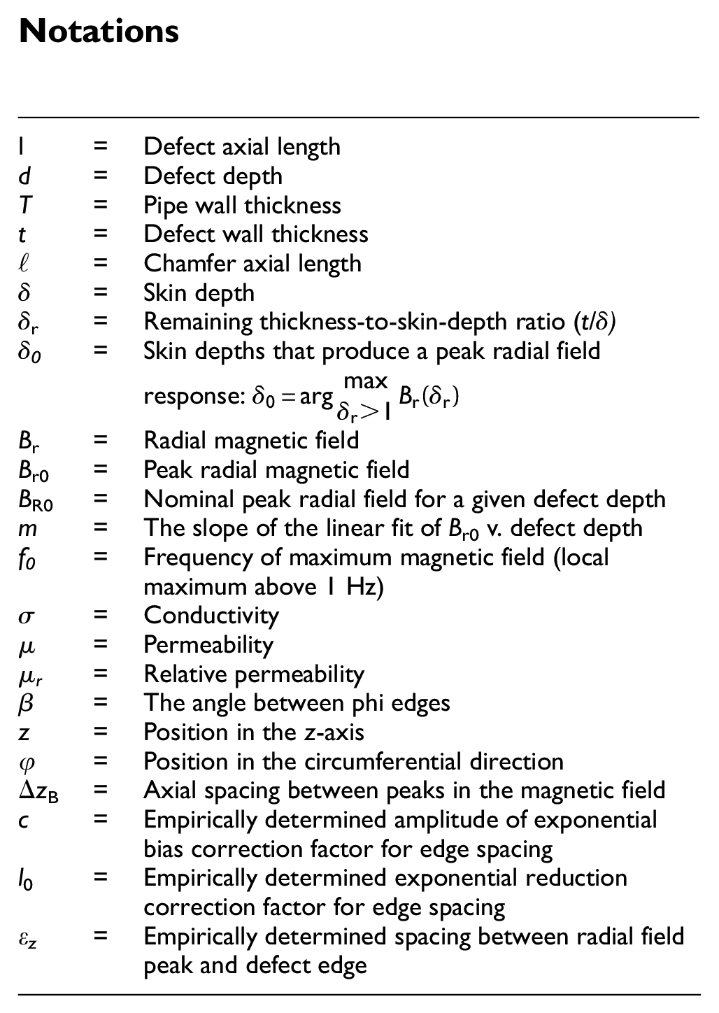
| l | = | Defect axial length |
| d | = | Defect depth |
| T | = | Pipe wall thickness |
| t | = | Defect wall thickness |
| ℓ | = | Chamfer axial length |
| δ | = | Skin depth |
| δ r | = | Remaining thickness-to-skin-depth ratio (t/δ) |
| δ0 | = | Skin depths that produce a peak radial field response: |
| B r | = | Radial magnetic field |
| B r0 | = | Peak radial magnetic field |
| B R0 | = | Nominal peak radial field for a given defect depth |
| m | = | The slope of the linear fit of Br0 v. defect depth |
| f0 | = | Frequency of maximum magnetic field (local maximum above 1 Hz) |
| σ | = | Conductivity |
| µ | = | Permeability |
| µr | = | Relative permeability |
| β | = | The angle between phi edges |
| z | = | Position in the z-axis |
| φ | = | Position in the circumferential direction |
| ΔzB | = | Axial spacing between peaks in the magnetic field |
| c | = | Empirically determined amplitude of exponential bias correction factor for edge spacing |
| l 0 | = | Empirically determined exponential reduction correction factor for edge spacing |
| εz | = | Empirically determined spacing between radial field peak and defect edge |
Declaration of conflicting interests
The author(s) declared no potential conflicts of interest with respect to the research, authorship, and/or publication of this article.
Funding
The author disclosed receipt of the following financial support for the research, authorship, and/or publication of this article: This work was supported by the New Zealand Ministry of Business, Innovation and Employment under the Endeavour grant RTVU1811.