Sage Journals: Discover world-class research

Abstract

Prognostics and health management (PHM) is becoming increasingly important as engineering structures and systems grow more complex. Many of these systems lack accurate physical models to describe their degradation, especially in unpredictable scenarios. To meet safety regulations, robust prognostic models are needed to transform sensor data into reliable predictions about a system’s remaining useful life (RUL). This study presents the adaptive hidden semi-Markov model (AHSMM), a novel probabilistic approach that enhances RUL prediction accuracy, uncertainty quantification (UQ), and reliability assessment compared to a long short-term memory (LSTM) model. A key contribution is an in-house experimental campaign involving glass fiber-reinforced polymer specimens subjected to fatigue loading and multiple impact events at different locations and time intervals. Unlike traditional models that rely on data from similar damage histories, the AHSMM is trained exclusively on unimpacted specimens and tested on multiply impacted ones, showcasing its adaptability to previously unseen conditions. The study also introduces a new prognostic performance measure tailored to AHSMM and develops a conditional reliability analysis for both AHSMM and LSTM predictions. Results demonstrate that AHSMM consistently outperforms LSTM across all evaluation metrics. It achieves a 24% lower RMSE over the full lifetime and superior UQ, with an average coverage of 0.79 compared to 0.17 for LSTM. Conditional reliability analysis further shows that AHSMM provides more accurate and stable reliability estimates as data accumulates. By capturing the degradation process and adapting to evolving conditions, AHSMM strengthens prognostic robustness. This study highlights the need for robust PHM models that can handle real-world uncertainties and contribute to advancements in the aerospace, automotive, and defense industries.

Keywords

PHM prognostics adaptive HSMM LSTM robustness impact damage composites

Introduction

Prognostics and health management (PHM) play a crucial role in ensuring operational safety, improving the reliability and availability of engineering assets, and reducing maintenance costs. A critical parameter in achieving these objectives is the prediction of remaining useful life (RUL), which is an output of the prognostics models.¹ Prognostics models are typically classified into three main types: physics-based, data-driven, and hybrid models.^2,3

Physics-based models describe the underlying degradation process using mathematical equations.⁴ However, these models often face limitations, as they tend to assume specific operational conditions and are typically applicable only to simple systems or components. In practice, most engineering systems and structures are much more complex, and physical models may not be available.⁵

Data-driven models, on the other hand, use historical degradation data from similar systems to make predictions.⁶ Supervised data-driven models, such as deep learning (DL) models, including long short-term memory (LSTM) networks and convolutional neural networks, have demonstrated high accuracy in various applications. However, these models are highly sensitive to the quality and quantity of training data, as well as to operational variability, unexpected phenomena, and environmental uncertainties common in real-world scenarios. Such challenges can lead to poor generalization and unreliable predictions.^7–9

In contrast, unsupervised data-driven models, such as stochastic models and Bayesian filters, offer a promising alternative for robust prognostics, particularly when labeled failure data are scarce or unavailable.^10,11 Additionally, stochastic models and Bayesian filters inherently provide uncertainty quantification (UQ), whereas UQ must be introduced separately in DL models through various mechanisms.¹² The probabilistic nature of stochastic models and Bayesian filters allows for RUL predictions with associated confidence levels.

Hybrid models seek to combine the strengths of both physics-based and data-driven approaches, aiming to improve prediction performance while reducing computational complexity. However, the practical implementation of these models remains challenging, limiting their widespread adoption.¹³

Due to the limitations of physics-based models, especially for complex systems, PHM has increasingly shifted its focus to data-driven approaches. In structural health monitoring (SHM), for example, data are typically collected using nondestructive testing techniques or networks of permanently attached sensors that gather real-time information about the degradation process.^14,15 However, the degradation of a structural component is heavily influenced by operational conditions such as environmental factors and load variations. Since it is impossible to account for all potential conditions during training, it becomes crucial to develop robust prognostics models that can maintain their performance even under unforeseen operational or environmental conditions.¹⁶

In industries such as aerospace, automotive, and defense, composite materials are widely used due to their desirable specific strength and stiffness, but they also present unique challenges for prognostics. These materials are not only vulnerable to impact damage, which can significantly reduce their load-bearing capacity, but their behavior is also complex and difficult to model, with no readily available physics-based models. Though considerable research has focused on diagnostic techniques to identify damage mechanisms,^17,18 fewer studies have directly addressed RUL prediction, particularly under realistic operational conditions. Most existing literature focuses on residual strength or damage progression estimation,^19–23 leaving a gap in RUL prediction research, which is critical for effective maintenance planning and mission operations.

Several studies have explored data-driven prognostics for composites under controlled conditions, where training and testing data are similar. For example, nonhomogeneous hidden semi-Markov models (NHHSMMs) have been used successfully to predict the RUL of composite structures based on acoustic emission (AE)²⁴ and Digital image correlation (DIC)²⁵ data from Carbon-fiber reinforced polymer (CFRP) open-hole coupons. Similarly, Gaussian process regression (GPR) has been employed for RUL prediction using health indicators (HI) derived from AE and Lamb waves, yielding reliable results under fixed operational conditions.^26,27

While these studies provide valuable insights, their applicability in real-world scenarios, where operational conditions often vary, is limited. A few studies have attempted to predict RUL under variable conditions. For instance, a physics-based Particle Filter model was used to estimate the RUL of composites subjected to impact tests, based on electromechanical behavior.¹⁹ However, this model is limited to monitoring electrical resistance in CFRP materials and does not account for fatigue loading, a key factor in load-bearing applications. Other research efforts have introduced Bayesian frameworks that correlate stiffness degradation with RUL,^28,29 but these models focus mainly on fatigue life estimation rather than addressing variable operational conditions. In the study by Cheng et al.,³⁰ a progressive damage model for residual strength and fatigue life of impacted glass fiber-reinforced polymer (GFRP) composite laminates after different loading conditions was developed. It was observed that the impacts had a greater effect on the fatigue strength of the composites when under compressive loads and that the loading sequence significantly affects damage evolution. Similarly, in the study by Zhao et al.,³¹ a model to predict the fatigue strength after impact of composite coupons was used. The model showed an average error of approximately 15%. The model parameters were fitted from the experimental data, and the only monitoring performed was the size of the impact damage via C-scan. These studies did not rely on experimental parameters, and no SHM systems were employed, making it less appealing for more complex systems where failure data may be unavailable. On the other hand, in the study by Zarouchas et al.,³² in situ high-speed impacts were performed on CFRP open hole coupons during tensile fatigue loading, and AE and DIC were used to monitor the behavior. Even though the two monitoring systems efficiently monitored the degradation process, no predictions of the fatigue life or strength were performed.

In recent years, there have been efforts to enhance the robustness of data-driven prognostics models under varying operational conditions and unexpected events. For example, a study examined RUL prediction of single stiffened composite panels using AE-based HIs, comparing the performance of GPR and Bayesian neural networks. Both models exhibited similar results, with GPR showing faster training times.³³ The same study also explored the use of strain-based HIs and GPR for predicting RUL,³⁴ while a similarity learning hidden semi-Markov model (HSMM) was employed to improve performance.³⁵ A further study was made by attempting to upscale their methodology in multistiffened composite panels using GPR and LSTM.³⁶ Their performance was only average, and it was noted that regression models are reliant on the input data. Another study introduced an adaptive NHHSMM, trained on open-hole composite specimens subjected to fatigue loading and tested on specimens that experienced an impact during fatigue loading.³⁷ These studies highlight the importance of prognostic models capable of modeling the degradation process rather than regressing on the SHM data.

The need for robust prognostics in composite materials is particularly urgent for two reasons. First, composites are vulnerable to impact damage, which can severely compromise their load-bearing capacity. Second, composites are susceptible to impact fatigue, which occurs when multiple impacts further degrade their structural integrity. While impact fatigue has been extensively reviewed,³⁸ it is often studied separately from fatigue loading, even though these two types of fatigue typically occur together, exacerbating the operational challenges of composite structures. The combined effect of these factors is further amplified when operational conditions vary, underscoring the importance of accurately estimating their impact on RUL.

This article presents a methodology for robust prognostic modeling of composite structures, focusing on model performance under complex and unpredictable scenarios. The adaptive HSMM (AHSMM) is proposed, incorporating an adaptation mechanism similar to that in the study by Eleftheroglou et al.³⁷ Unlike prior studies that considered only single-impact events, this work introduces an experimental campaign involving multiple impacts applied at different locations during fatigue loading. This setup better reflects operational conditions in defense and aerospace applications, where systems are exposed to repeated and varied impact events.

To capture these events, SHM sensors are employed. From the sensor data, statistical features are extracted to derive a degradation signal, which is then used as input to the AHSMM for predicting the RUL of multiply impacted composite coupons. The complete framework is illustrated in Figure 1.

Figure 1.

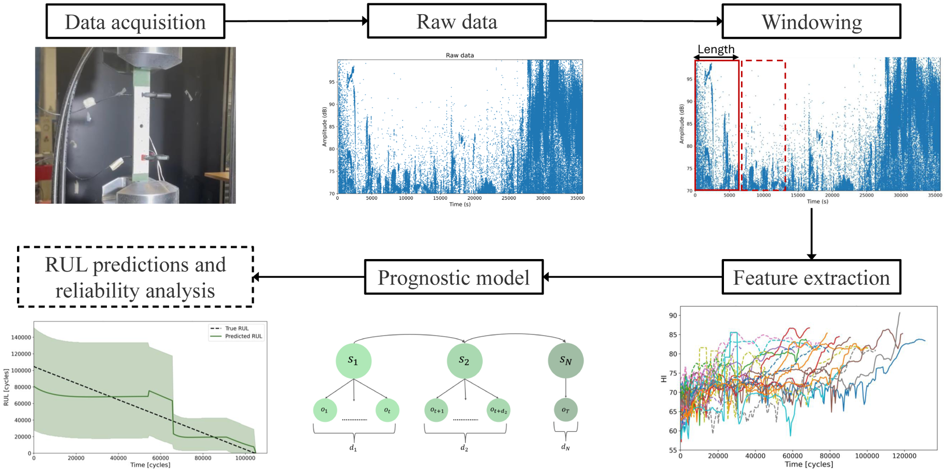
Prognostic framework using SHM data and AHSMM for RUL prediction of multiimpacted composite structures. SHM: structural health monitoring; RUL: remaining useful life; AHSMM: adaptive hidden semi-Markov model.

The data division strategy trains the model on unimpacted specimens and evaluates it on multiply impacted ones. This approach is crucial for assessing the model’s ability to adapt to previously unseen damage conditions.

Accordingly, this study makes three key contributions:

A new prognostic performance measure tailored to the AHSMM model.

A new case study for prognostics through an experimental campaign with multiple impacts in different locations in GFRP composite structures.

A conditional reliability analysis for direct evaluation of RUL prediction uncertainty from both AHSMM and LSTM models.

The remainder of the article is structured as follows: “Methodologies” section presents the basic principles of the methodologies employed for the RUL estimations and conditional reliability, and “Case study: unexpected impact events” section describes the case study that is used to evaluate the methodologies. “Results and discussion” section is split into two sections, presenting the main results of the article and a discussion about the need for robust prognostics. Finally, the conclusions are presented in “Conclusions” section.

Methodologies

This section outlines the methodology used to develop the AHSMM model and the LSTM model, which is used as a comparison point for the RUL and conditional reliability estimations. The AHSMM is an adaptive extension of the well-established hidden semi-Markov model (HSMM),³⁹ while the adaptive extension of the model is based on the methodology used in the study by Eleftheroglou et al.³⁷ The LSTM is based on the architecture presented in the study by Asif et al.⁴⁰

Adaptive hidden semi-Markov model

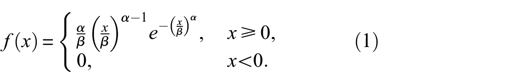
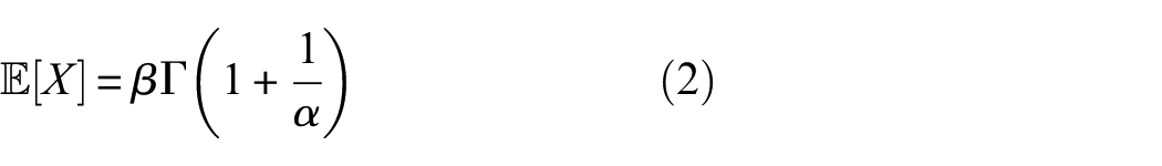
The HSMM is an extension of the hidden Markov model (HMM)⁴¹ with the inclusion of a variable sojourn time for each damage state. For each damage state, a number of observations are emitted depending on the sojourn time of the given damage state. For this study, the sojourn time of each damage state is given by a Weibull distribution. The parameters of the HSMM are described below:

N: number of damage states. The set of damage states is denoted as $S = {S_{1}, S_{2}, \dots, S_{N}}$ . Each damage state represents a level of degradation.

M: number of distinct observation symbols. The observation process is modeled with a Gaussian distribution, therefore, the space consists of all the real numbers.

λ: transition rate function.It describes the degradation process that follows a rate function, denoted by λ. For this study, the λ function corresponds to the Weibull distribution, which is commonly used in reliability theory.

To train the HSMM, the Expectation–Maximization algorithm is used. Details of this procedure can be found in the study by Shun-Zheng et al.⁴² However, some assumptions are made to use this model for prognostics.

Initial state: the model starts in the first damage state. Therefore, the engineering system is assumed to always start as good as new.

Transitions: only left-to-right transitions are allowed. This means that the model can only transit to a neighboring state or stay in the current state. Therefore, it is assumed that the engineering system does not recover health and that it has to go through all the states before reaching failure.

Final state: the final state of the HSMM is observable, and it represents failure. In the final state, only one observation value is emitted.

Finally, Figure 2 presents a representation of the HSMM incorporating the assumptions made for prognostics.

Figure 2.

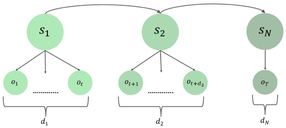
HSMM representation. HSMM: hidden semi-Markov model.

As previously mentioned, the model AHSMM is an adaptive extension of the HSMM. The overall adaptation process is illustrated as a flowchart in Figure 3. During the testing phase, the adaptation is triggered once a transition from damage state $S_{i}$ to damage state $S_{i + 1}$ occurs. The sojourn time of the damage state $S_{i}$ is then $T_{i}$ and is compared to the expected value from the Weibull distribution for that damage state, $E_{i}$ . The Weibull distribution is defined in Equation (1), in which $α$ is the shape parameter and $β$ is the scale parameter. The expected value is defined in Equation (2).

f (x) = {\begin{matrix} \frac{α}{β} {(\frac{x}{β})}^{α - 1} e^{- {(\frac{x}{β})}^{α}}, & x \geq 0, \\ 0, & x < 0 . \end{matrix}

(1)

E [X] = β Γ (1 + \frac{1}{α})

(2)

Figure 3.

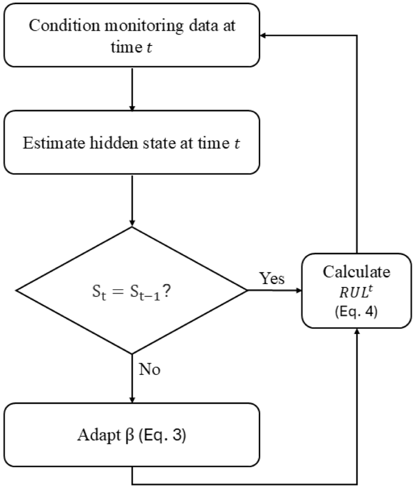
Flowchart of the adaptation process.

A ratio between $T_{i}$ and $E_{i}$ of the current state, $S_{i}$ , is calculated and used as a resampling factor ( $R_{f}$ ) for the sojourn time of the next damage state, $S_{i + 1}$ . To resample the sojourn time of $S_{i + 1}$ , the scale parameter is adapted since it can shift the Weibull distribution to have shorter and longer sojourn times. The adapted scale parameter for the state $S_{i + 1}$ is denoted as $β_{i + 1}^{*}$ and is defined in Equation (3). Thus, the Weibull distribution for $S_{i + 1}$ is defined by the parameters ( $α_{i + 1}, β_{i + 1}^{*}$ ) since the shape parameter $α$ is not adapted and remains the same as the one calculated during training.

β_{i + 1}^{*} = \frac{E_{i + 1} R_{f}}{Γ (1 + \frac{1}{α_{i + 1}})}

(3)

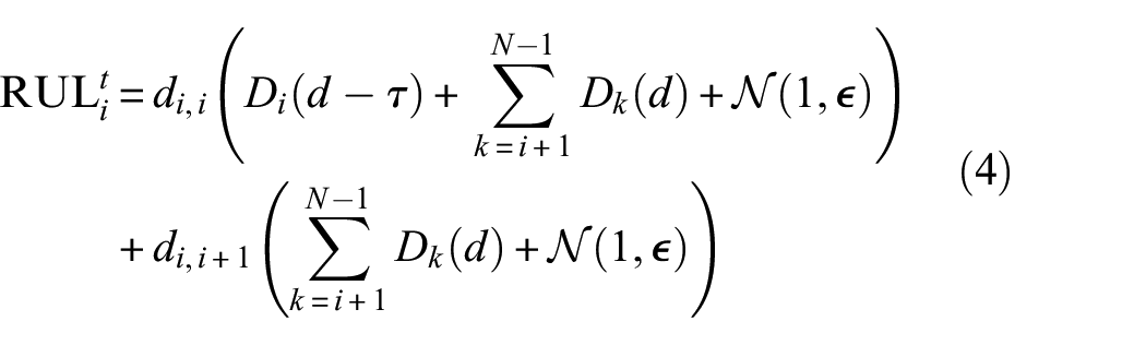
For RUL prediction, a time-dependent prognostic measure is used, following the framework in the study by.^39,43 This formulation provides a probability distribution for the RUL that evolves with time spent in the current damage state.

The variables in Equations (4)–(6) are defined as follows:

$D_{i} (d)$ : The probability density function (pdf) of the sojourn time in damage state $i$ , evaluated at time $d$ .

τ: Time already spent in the current state i; thus, $D_{i} (d - τ)$ accounts for elapsed time, making the estimate time-dependent.

$d_{i, i + 1} = P (d \leq τ ∣ S_{t} = i)$ : Probability of transitioning to the next damage state $i + 1$ within time $d$ .

$d_{i, i} = 1 - d_{i, i + 1}$ : Probability of remaining in the current state beyond time $d$ .

$N (1, ϵ)$ : Gaussian noise term accounting for uncertainty in predictions.

The resulting RUL expression gives a probability distribution per time step, and 95% confidence intervals are computed using the cumulative distribution function (CDF). Since the AHSMM is a stochastic model, the uncertainty reflected in the pdf corresponds to the aleatoric uncertainty with the added uncertainty propagation that comes from the prognostic measure. Aleatoric uncertainty refers to the inherent variability or randomness in a system or process that cannot be reduced, even with more information or data:

\begin{matrix} {RUL}_{i}^{t} = d_{i, i} (D_{i} (d - τ) + \sum_{k = i + 1}^{N - 1} D_{k} (d) + N (1, ϵ)) \\ + d_{i, i + 1} (\sum_{k = i + 1}^{N - 1} D_{k} (d) + N (1, ϵ)) \end{matrix}

(4)

d_{i, i + 1} = P (d \leq τ | S_{t} = i)

(5)

d_{i, i} = 1 - d_{i, i + 1}

(6)

Conditional reliability is defined as the probability that the system remains operational at a future time $t$ , given that the lifetime $L$ exceeds $t$ ( $L > t$ ), that $t$ is beyond the current time $t_{p}$ , that the system has not yet reached its end of life ( $L > t_{p}$ ), and is conditioned on the observed test data $y_{1 : t_{p}}$ and the prognostic model $M$ . Mathematically, conditional reliability is expressed by the CDF of RUL, as shown in Equation (7):

\begin{matrix} R (t + t_{p} | y_{1 : t_{p}}, M) = 1 - P (RU L^{t_{p}} \leq t | y_{1 : t_{p}}, M) \end{matrix}

(7)

Long short-term memory

The LSTM has been widely used in prognostics, given its high accuracy in predicting RUL, since it can learn temporal features in time-series data. The LSTM is a supervised model, and it maps the HI values to the labels (regression), which are RUL values in the prognostics case.

Figure 4 presents the architecture used for this article. The architecture only uses two LSTM layers, given the low amount of data available to train, and that only one feature is available. The model’s hyperparameters are shown in Table 1 and are chosen based on a random search using Keras Tuner. The input for the LSTM consists of windows of 10 samples. This choice is driven by the need for the LSTM to receive inputs of consistent length and to be utilized in an online manner, necessitating the data to be windowed; therefore, the dense layer needs to have 10 units.

Figure 4.

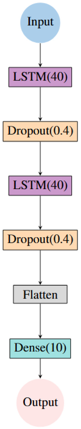
LSTM architecture for prognostics. LSTM: long short-term memory.

Table 1.

LSTM hyperparameters.

Hyperparameter	Value
Number of hidden units	40
Dropout probability	0.4
Learning rate	0.001
Batch size	64
Optimizer	Adam
Loss function	MSE

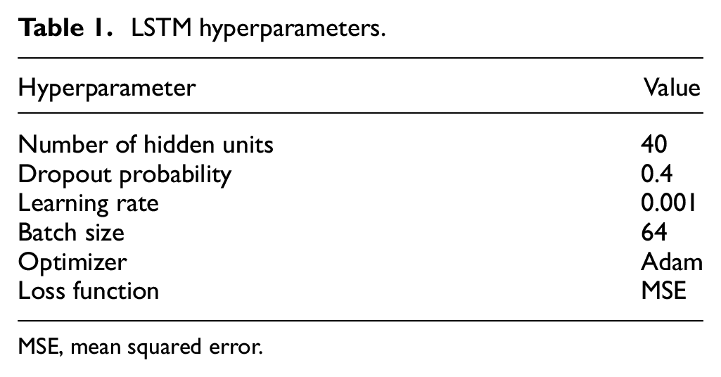
MSE, mean squared error.

To account for uncertainty, the Monte Carlo (MC) dropout technique is utilized, which accounts for epistemic uncertainty.⁴⁴ Epistemic uncertainty is the uncertainty that arises from a lack of knowledge or information about a system or process, and can potentially be reduced with more data or better understanding. For this study, the number of forward passes to account for uncertainty equals 100 since it is the standard number in the literature. Similar to AHSMM, the conditional reliability for the LSTM is calculated in the same way as shown in Equation (7). It is worth noting that the pdf of RUL for the LSTM is defined as a Gaussian distribution determined from the samples taken with the MC dropout technique.

Case study: unexpected impact events

The proposed model is evaluated in a case study involving (multiple) impacts during constant amplitude tensile fatigue tests. An experimental campaign is conducted on GFRP specimens subjected to both fatigue loading and multiple impacts. The case study focuses on creating unexpected events that can occur during operation and evaluates the capabilities of the model to handle short-term unexpected events similar to the study by Eleftheroglou et al.³⁷

Specimen specifications and experiment definition

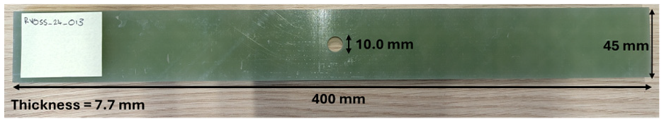
GFRP coupons were manufactured from SL90–T0/EGL, with a nominal length of 400 mm and a width of 45 mm. An eight-ply quasi-isotropic layup of $[0 / + 45 / 90 / - 45]_{S}$ was used, leading to a nominal thickness of 7.7 mm (Figure 5). A 10 mm hole was drilled at the center of the coupons using a diamond drill bit to minimize damage. Quasi-static tensile tests were performed to determine the tensile failure load, which averaged 69 kN, using a 1.5 mm/min loading rate. This value guided the selection of the load level during the subsequent tensile fatigue tests.

Figure 5.

GFRP coupon depiction and dimensions. GFRP: glass fiber-reinforced polymer.

The fatigue tests comprised constant amplitude tension-tension fatigue where the load was fixed at 50% of the average tensile failure load, the load ratio at 0.1, and the frequency at 4 Hz. The tests were run in an MTS hydraulic machine with a 250 kN load capacity. The fatigue was interrupted every 500 cycles, for 2 s, allowing pictures to be taken at the maximum load to inspect damage progression and failure during postprocessing visually. Additionally, the entirety of the fatigue loading is monitored using Vallen VS900-M AE sensors, paired with a four-channel AMSY-6 acquisition system and an external pre-amplifier of 34 dB. To reduce the external noise and hits not associated with degradation, a 50-dB threshold was set.

Two types of tests were conducted: fatigue testing (until failure) of unimpacted specimens, and fatigue testing with in situ impacts at various time intervals, while the specimens were loaded with the mean value of the fatigue loading. Impacts were performed via an in-house gas gun, which is shown in Figure 6. As shown in Figure 7, the hemispherical aluminum projectile is attached to a plastic cylinder that matches the barrel’s radius. The length of the projectile (including the aluminum tip) was 35 mm, and the diameter was 25 mm. The total weight of the projectile is approximately 16 g. The purpose of this shape and design is to reduce spinning effects inside the barrel and ensure a precise impact location. The impact pressure ranged from 1.2 to 1.5 bar. To protect the AE sensors, they were removed during the impact and re-attached before restarting the fatigue.

Figure 6.

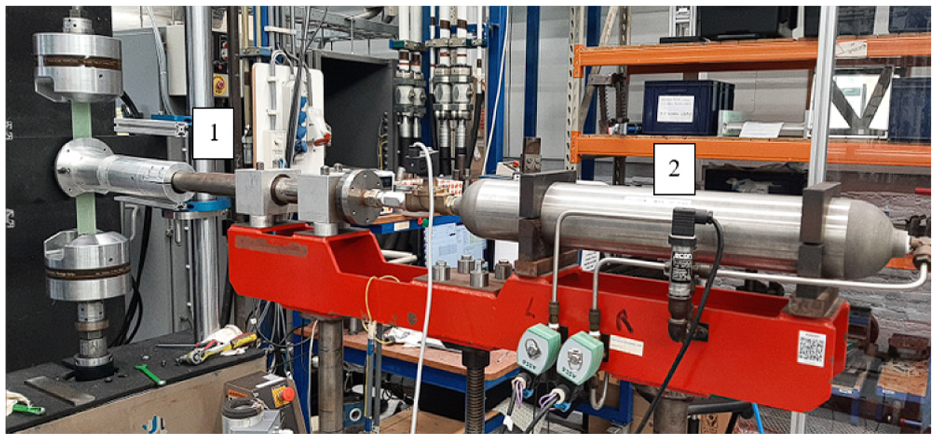
Impact gas gun setup.

Figure 7.

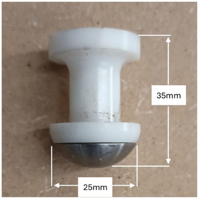
Projectile.

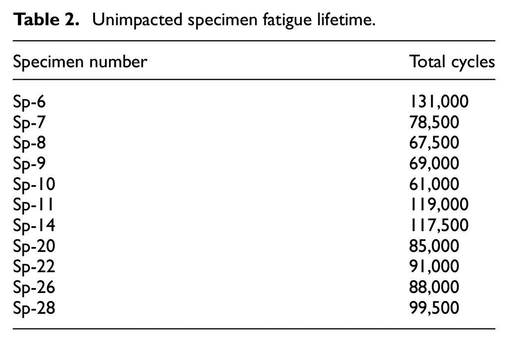
The goal of the impact(s) is to simulate unexpected events during fatigue testing, which can commonly occur during the operation of a structure. These events affect structural integrity and the degradation process, resulting in changes in the fatigue life. Additionally, the impacts present a challenge that is used to evaluate the robustness of the models and their ability to adapt their predictions to the altered degradation process. The fatigue life of unimpacted specimens is provided in Table 2, while Table 3 specifies the impact conditions and reports the lifetimes for impacted specimens. Failure time is derived during postprocessing; thus, lifetimes are reported as the time the picture is captured. The total collapse was the result of the specimens snapping in two, while from visual inspection, failure is considered at the time separation initiates, which is accompanied by a significant stiffness drop observed from the load-displacement data.

Table 2.

Unimpacted specimen fatigue lifetime.

Specimen number	Total cycles
Sp-6	131,000
Sp-7	78,500
Sp-8	67,500
Sp-9	69,000
Sp-10	61,000
Sp-11	119,000
Sp-14	117,500
Sp-20	85,000
Sp-22	91,000
Sp-26	88,000
Sp-28	99,500

Table 3.

Impacted specimen information and lifetime.

Specimen number	Impact pressure (bar) × number	Time of impact (cycles)	Total cycles
Sp-12	1.2 × 1	20k	75,500
Sp-15	1.2 × 2	20k, 40k	101,000
Sp-16	1.2 × 2	20k × 2	75,000
Sp-17	1.5 × 2	5k, 10k	61,500
Sp-18	1.5 × 2	10k × 2	90,000
Sp-19	1.5 × 3	5k, 10k, 15k	23,500
Sp-21	1.5 × 2 and 1.0 × 1	5k, 10k, 15k (1 bar)	32,500
Sp-23	1.5 × 3	5k × 3	23,000
Sp-24	1.5 × 1	5k	104,500
Sp-25	1.5 × 3	5k, 10k (5 cm below hole), 15k	48,500
Sp-27	1.5 × 3	5k, 10k, 15k (all 5 cm below hole)	79,500

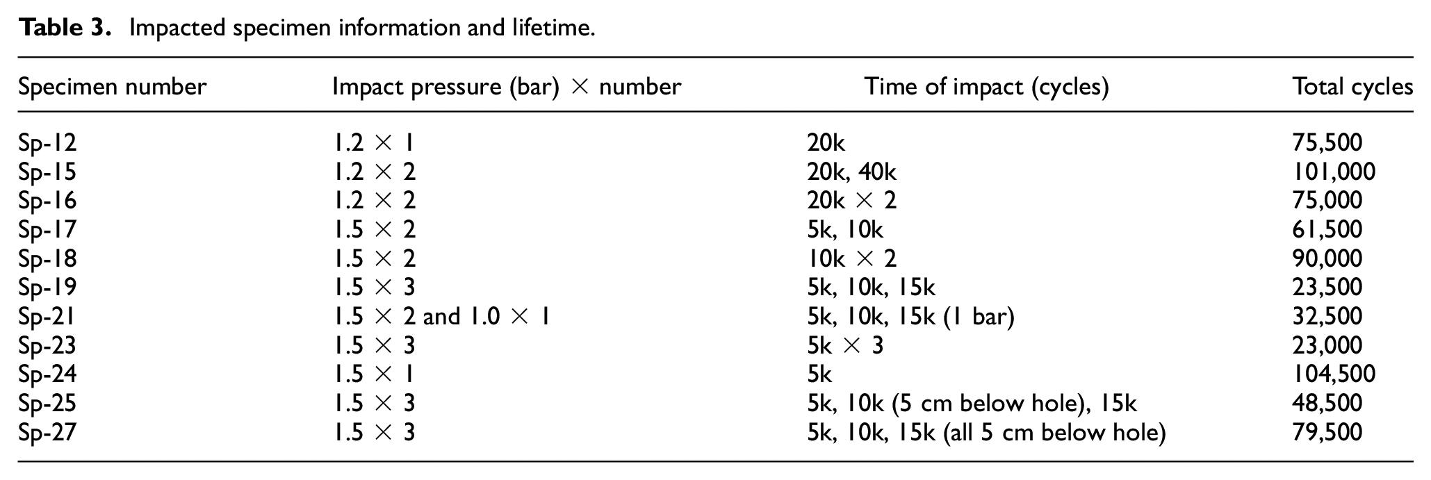
Impacts were performed at the location of the hole unless specified otherwise. In Table 3, simultaneous impacts are denoted with “×” (e.g., “10k × 2” indicates two consecutive impacts at cycle 10,000), whereas sequential impacts are separated by commas (e.g., “5k, 10k, 15k” represent impacts occurring at 5000, 10,000, and 15,000 cycles, respectively). The total cycles column reflects the lifetime of each specimen under the specified conditions.

As observed in Tables 2 and 3, impact damage does not necessarily reduce fatigue life; in some cases, impacted specimens outlast unimpacted ones. This outcome may result from stress redistribution around the drilled hole in the quasi-isotropic layup. Additionally, impact-induced delaminations or fiber breakage could modify local stress fields, potentially reducing stress concentrations.

Data preprocessing and feature extraction:

The AE data collected during the tests were used to extract informative features for the RUL estimation. 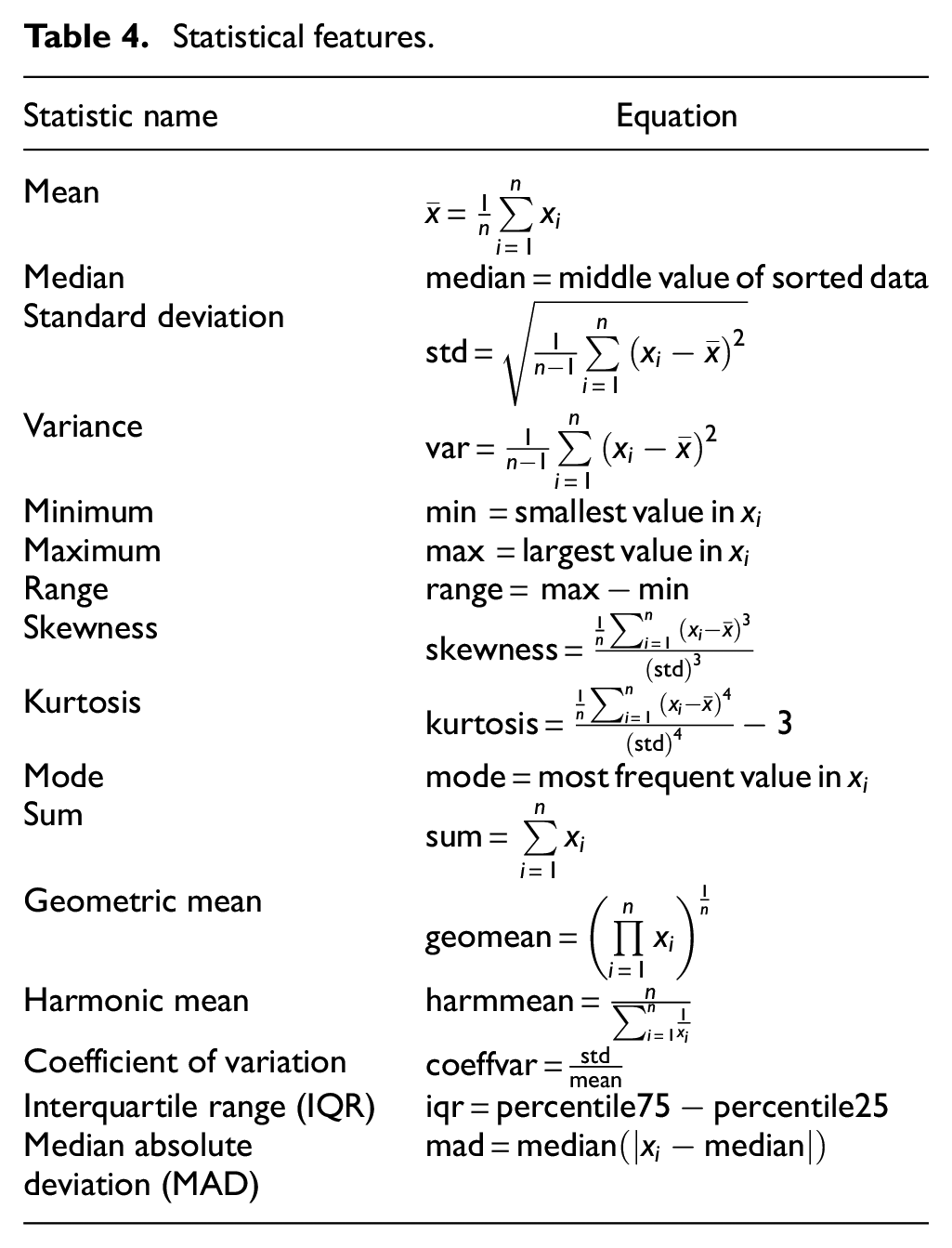In the first step the low-level AE features, including amplitude, duration, rise time, energy, counts, and so on, are windowed using a nonoverlapping 500-cycle window since it has been demonstrated that cumulative features are not always representative of the degradation and suffer from poor prognosability (dependent on running time).²⁵ The window size was chosen arbitrarily based on the cycles that the photos were taken. In the second step, since the low-level features are not sensitive enough to degradation, statistical features were calculated for each window in both the time and frequency domains in an attempt to identify degradation-sensitive features.^45,46 The mathematical formulation of these statistical features is demonstrated in Table 4, where $x_{i}$ is a data point in each window with a size of $n$ samples. Transformation to the frequency domain was done via the fast Fourier transform.

Table 4.

Statistical features.

Statistic name	Equation
Mean	$\bar{x} = \frac{1}{n} \sum_{i = 1}^{n} x_{i}$
Median	$median = middle value of sorted data$
Standard deviation	$std = \sqrt{\frac{1}{n - 1} \sum_{i = 1}^{n} {(x_{i} - \bar{x})}^{2}}$
Variance	$var = \frac{1}{n - 1} \sum_{i = 1}^{n} {(x_{i} - \bar{x})}^{2}$
Minimum	$min = smallest value in x_{i}$
Maximum	$max = largest value in x_{i}$
Range	$range = max - min$
Skewness	$skewness = \frac{\frac{1}{n} \sum_{i = 1}^{n} {(x_{i} - \bar{x})}^{3}}{{(std)}^{3}}$
Kurtosis	$kurtosis = \frac{\frac{1}{n} \sum_{i = 1}^{n} {(x_{i} - \bar{x})}^{4}}{{(std)}^{4}} - 3$
Mode	$mode = most frequent value in x_{i}$
Sum	$sum = \sum_{i = 1}^{n} x_{i}$
Geometric mean	$geomean = {(Π_{i = 1}^{n} x_{i})}^{\frac{1}{n}}$
Harmonic mean	$harmmean = \frac{n}{\sum_{i = 1}^{n} \frac{1}{x_{i}}}$
Coefficient of variation	$coeffvar = \frac{std}{mean}$
Interquartile range (IQR)	$iqr = percentile 75 - percentile 25$
Median absolute deviation (MAD)	$mad = median (\| x_{i} - median \|)$

Apart from the statistical features in the time and frequency domains, principal component analysis (PCA) is performed in both domains, including all primary (low-level AE features recorded by the AE system) and secondary features (statistical features extracted in the previous step). The PCA model, similar to the study by Loukopoulos et al.,⁴⁷ is created using only a healthy subset of the data, which consists of the time of the first impact or 10,000 cycles if no impact is performed (chosen arbitrarily), and then the entire dataset is transformed into the principal component space. The cumulative squared reconstruction residual (Q) and Hotelling’s T² are calculated and, to improve prognosability, the natural logarithm is applied.

The suitability of the extracted features was evaluated using the sum of Spearman rank monotonicity (Equation (8)), prognosability (Equation (9)), and trendability (Equation (10)).⁴⁸

Mo = \frac{1}{M} \sum_{j = 1}^{M} | corr (rank (x_{j}), rank (t_{j})) |

(8)

\Pr = \exp (- \frac{{std}_{j} (x_{j} (N_{j}))}{{mean}_{j} | x_{j} (1) - x_{j} (N_{j}) |}), j = 1, \dots, M

(9)

Tr = \min_{j, k} | \frac{cov (x_{j}, x_{k})}{σ_{x_{j}} σ_{x_{k}}} |, j, k = 1, 2, \dots, M

(10)

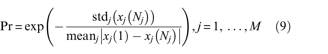
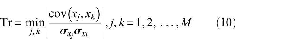
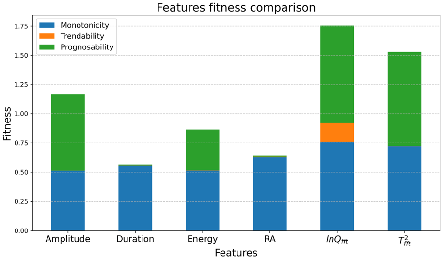
As demonstrated in Figure 8, the raw features (amplitude, duration, frequency, and rise-time/amplitude) consistently exhibit poor performance across all evaluation metrics. Among the extracted features, $lnQ$ calculated in the frequency domain ( $\ln Q_{fft}$ ) demonstrates superior performance according to the aforementioned metrics. Notably, $\ln Q_{fft}$ exhibits high monotonicity and prognosability, though it shows extremely low trendability.

Figure 8.

Comparison of raw and top two best features based on monotonicity, trendability, and prognosability metrics.

It is also worth highlighting that when compared to prognostic feature optimization studies,^34,46,49 the prognostic feature shows only average performance in the combined metrics. Purposefully, further investigation is not performed to demonstrate that the proposed prognostic model is capable of providing good results even with average prognostic features, and optimization of the degradation feature is outside the scope of the article.

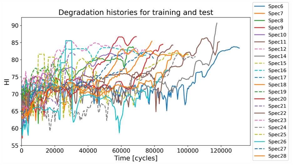
The behavior of $\ln Q_{fft}$ for the different specimens is shown in Figure 9. This feature will be used as the input to train the prognostic models and predict the RUL. The data are split into training and testing sets, with the training data consisting solely of specimens without impact, and the testing data including only specimens with impact. This approach allows for evaluating the proposed methodology on unseen events during training and demonstrates its robustness in adapting to such events during operation.

Figure 9.

Degradation histories of train and test set using feature $\ln Q_{fft}$ .

In addition, Figure 10 shows the degradation histories of selected test specimens, along with the corresponding times of impact. Impact times are indicated with circles, and a larger circle denotes that two impacts occurred within the same cycle. For better visual clarity, only four representative degradation histories are shown. It can be observed that the impact event does not necessarily alter the behavior of the degradation feature, providing a clear indication of damage initiation.

Figure 10.

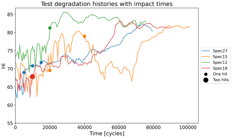
Test degradation histories with marked times of impacts.

Results and discussion

The proposed AHSMM was trained exclusively on data from specimens that were not subjected to in situ impacts. As a result, unexpected impact events were excluded from the training process and only introduced during testing. The same training strategy was applied to the LSTM model, which is used here for performance comparison. A Q-Q plot of the RUL predictions from both models is shown in Figure 11. The plot reveals that both models exhibit reduced accuracy during the early life cycles. However, as the specimens approach end-of-life, the AHSMM aligns more closely with the ideal distribution than the LSTM, highlighting the benefits of its adaptiveness. Given this performance distinction, only the RUL predictions from the AHSMM are presented in the following analysis for clarity.

Figure 11.

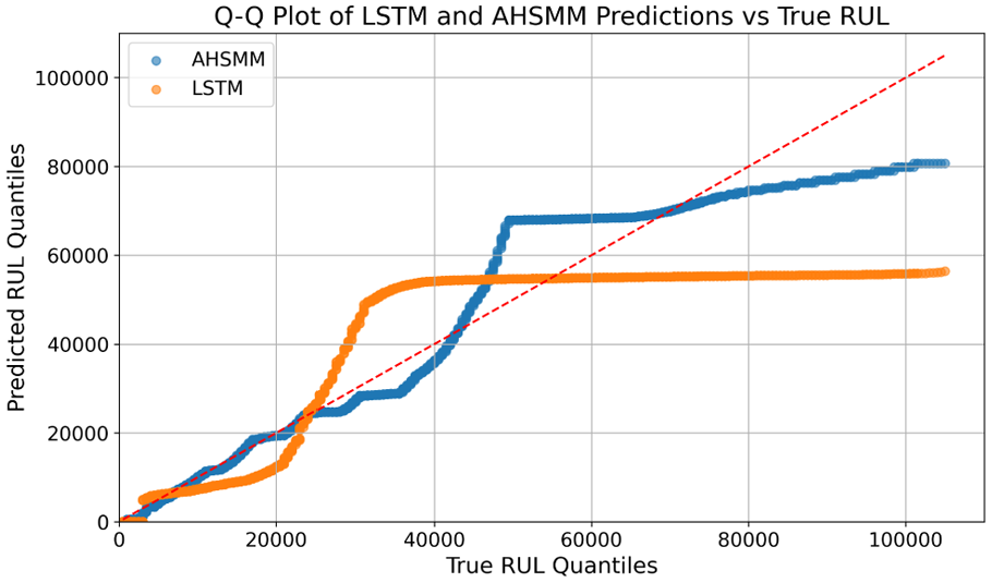
Q-Q plot of AHSMM and LSTM predictions for all test samples. AHSMM: adaptive hidden semi-Markov model; LSTM: long short-term memory.

To illustrate the model’s performance, three RUL plots are presented in Figure 12, corresponding to the specimens with the shortest, average, and longest fatigue life within the test set. The comprehensive summary of results across all test specimens is provided in Tables 5, 6, and 7.

Figure 12.

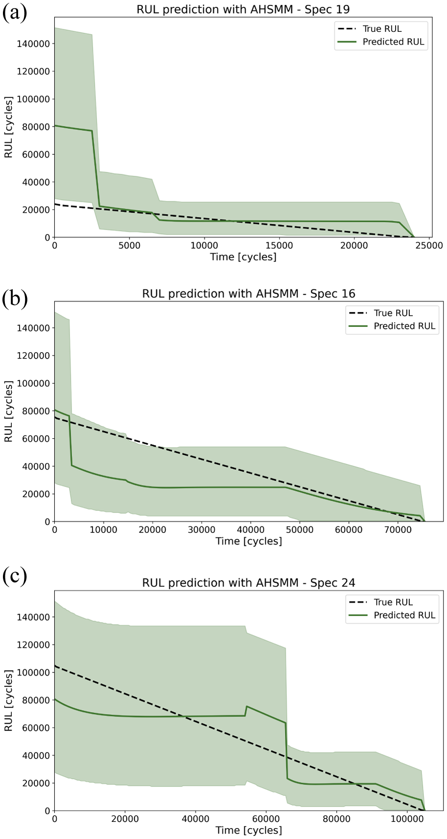
RUL predictions with the AHSMM: (a) left outlier, (b) inlier, and (c) right outlier. (a) RUL prediction for the test specimen with the shortest lifetime (SP-19). (b) RUL prediction for the test specimen with average lifetime (SP-16). (c) RUL prediction for the test specimen with the longest lifetime (SP-24). RUL: remaining useful life; AHSMM: adaptive hidden semi-Markov model.

Table 5.

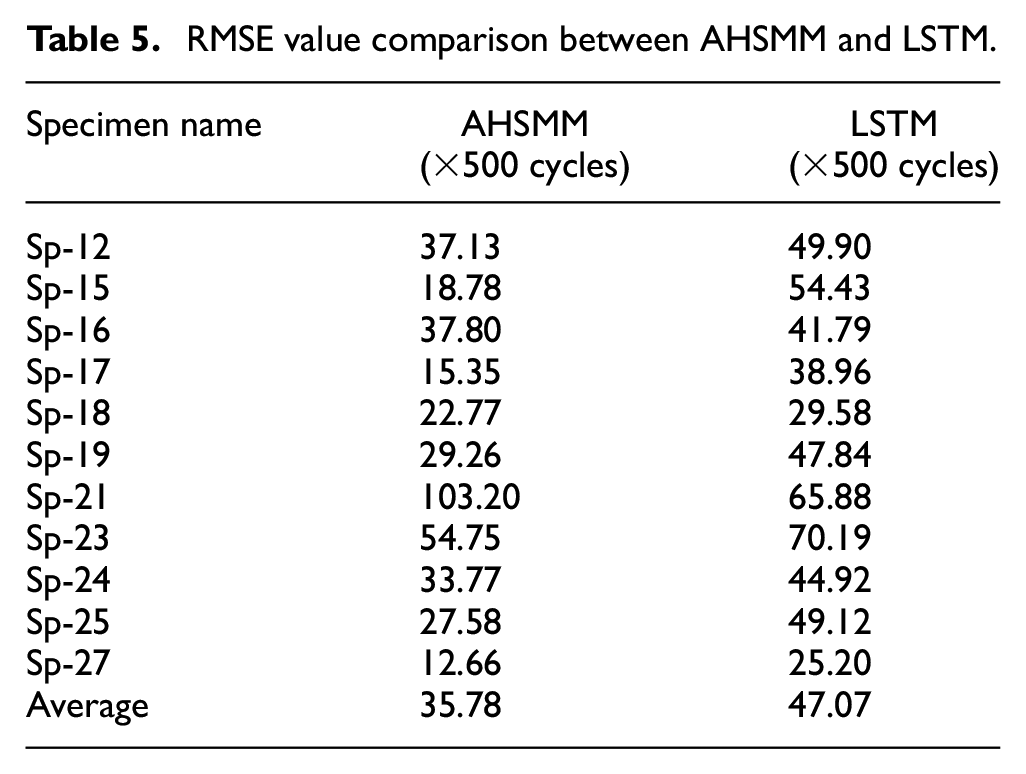
RMSE value comparison between AHSMM and LSTM.

Specimen name	AHSMM (×500 cycles)	LSTM (×500 cycles)
Sp-12	37.13	49.90
Sp-15	18.78	54.43
Sp-16	37.80	41.79
Sp-17	15.35	38.96
Sp-18	22.77	29.58
Sp-19	29.26	47.84
Sp-21	103.20	65.88
Sp-23	54.75	70.19
Sp-24	33.77	44.92
Sp-25	27.58	49.12
Sp-27	12.66	25.20
Average	35.78	47.07

Table 6.

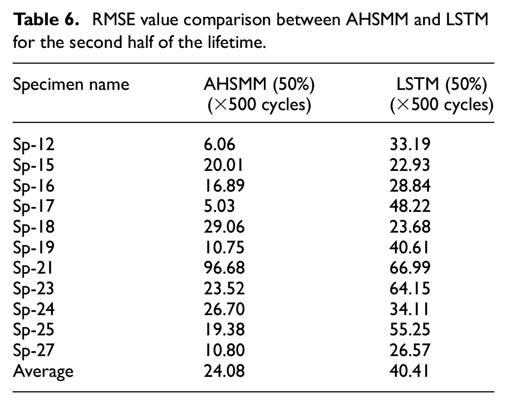
RMSE value comparison between AHSMM and LSTM for the second half of the lifetime.

Specimen name	AHSMM (50%) (×500 cycles)	LSTM (50%) (×500 cycles)
Sp-12	6.06	33.19
Sp-15	20.01	22.93
Sp-16	16.89	28.84
Sp-17	5.03	48.22
Sp-18	29.06	23.68
Sp-19	10.75	40.61
Sp-21	96.68	66.99
Sp-23	23.52	64.15
Sp-24	26.70	34.11
Sp-25	19.38	55.25
Sp-27	10.80	26.57
Average	24.08	40.41

Table 7.

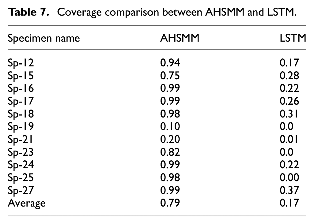
Coverage comparison between AHSMM and LSTM.

Specimen name	AHSMM	LSTM
Sp-12	0.94	0.17
Sp-15	0.75	0.28
Sp-16	0.99	0.22
Sp-17	0.99	0.26
Sp-18	0.98	0.31
Sp-19	0.10	0.0
Sp-21	0.20	0.01
Sp-23	0.82	0.0
Sp-24	0.99	0.22
Sp-25	0.98	0.00
Sp-27	0.99	0.37
Average	0.79	0.17

Unexpected events typically, but not always, lead to a reduction in the overall fatigue life of a specimen. This effect is particularly evident in Figure 12(a), which corresponds to the specimen with the shortest lifetime. Initially, the model significantly overestimates the true RUL; however, after adaptation, the AHSMM refines its predictions to accurately estimate the true RUL. Meanwhile, the specimen with the longest lifetime (Figure 12(c)) shows consistency between the predicted and actual RUL, as its lifespan falls within the range learned from the training data. Similarly, the predicted RUL for the specimen with an average lifetime (Figure 12(b)) aligns closely with the true RUL during the latter part of its life cycle.

Two key evaluation metrics are used: Root mean squared error (RMSE) and coverage. RMSE quantifies the error between the true and predicted mean RUL, while coverage assesses UQ by measuring the proportion of true RUL values that fall within the predicted confidence intervals. Specifically, if $y_{t}$ represents the true RUL value at time step $t$ and $[l_{t}, u_{t}]$ denotes the predicted lower and upper bounds, the coverage for a single prediction $C_{t}$ equals $1$ if $l_{t} \leq y_{t} \leq u_{t}$ ; otherwise, it equals $0$ . For a complete degradation history of length $T$ , the coverage metric is defined in Equation (11).

\begin{matrix} Coverage = \frac{1}{T} \sum_{t = 1}^{T} C_{t} \end{matrix}

(11)

Table 5 compares RMSE values between AHSMM and LSTM. The AHSMM consistently achieves lower RMSE values across all tested specimens, expect for SP-21, demonstrating its superior predictive performance. The adaptive module within AHSMM significantly enhances accuracy as new data become available. In particular, when evaluating performance over the second half of the lifetime of each specimen (Table 6), the AHSMM shows a substantial reduction in RMSE, highlighting the model’s capability to refine its estimates as more degradation data is collected.

Coverage results shown in Table 7, further emphasize the robustness of AHSMM. The AHSMM achieves an average coverage of 0.79, significantly outperforming the LSTM, which only achieves 0.17. This indicates that the AHSMM provides more reliable UQ, ensuring that the true RUL values are better captured within the confidence intervals.

To further analyze model performance from a conditional reliability perspective, Figure 13 presents reliability comparisons between AHSMM and LSTM at different time steps. At the beginning of the degradation cycle (Figure 13(a)), the conditional reliability estimates for both models exhibit higher uncertainty. However, as more data become available, AHSMM adapts effectively, providing more precise reliability estimates, as shown in Figure 13(b) and (c). In contrast, LSTM struggles to maintain accurate reliability estimates.

Figure 13.

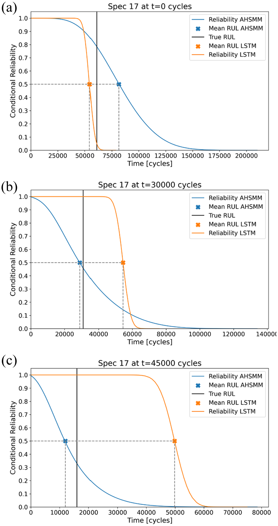
Conditional reliability comparison between AHSMM and LSTM for SP-17. (a) Conditional reliability at t = 0 cycles. (b) Conditional reliability at t = 30,000 cycles. (c) Conditional reliability at t = 45,000 cycles. AHSMM: adaptive hidden semi-Markov model; LSTM: long short-term memory.

Discussions

This study underscores the need for robust prognostic models capable of handling unexpected operational conditions. The results demonstrate that state-of-the-art machine learning models like LSTM have a significant decrease in their prognostic performance when unexpected events occur, particularly for specimens with significantly shorter lifetimes than those observed in the training set. This limitation is inherent in models that rely heavily on training data distributions, which may not adequately account for rare or unexpected events.

The need for robust and adaptive prognostic models becomes even more apparent in applications operating under harsh and dynamic environments, such as aerospace or defense applications. For example, civil aircraft typically operate under predefined conditions for each flight cycle, but unexpected weather phenomena or bird strikes can alter these conditions, requiring real-time adaptation of RUL predictions to enhance condition-based maintenance planning. This requirement is even more critical for military aircraft, where rapid maneuvering and unpredictable conditions highlight the need for real-time awareness of structural health and mission readiness.

To establish a robust framework for PHM, adaptive models such as AHSMM are essential. A crucial component of such a framework is UQ, which is categorized into aleatoric and epistemic uncertainty. Aleatoric uncertainty stems from the inherent randomness in data, while epistemic uncertainty arises due to a lack of knowledge or model limitations.⁵⁰ As discussed in “Methodologies” section, AHSMM effectively captures and propagates aleatoric uncertainty, whereas LSTM models address only epistemic uncertainty using techniques such as MC Dropout.

Results from AHSMM demonstrate that the confidence intervals generated by the model generally encompass the true RUL, although with wide intervals. This aligns with findings in other stochastic prognostic models, highlighting the importance of uncertainty management. Effective uncertainty management⁵¹ can minimize the impact of uncertainties on RUL predictions, thereby improving decision-making robustness. Future research should explore advanced techniques for uncertainty management to refine confidence intervals and enhance the accuracy of RUL predictions, ultimately strengthening the robustness of PHM frameworks.

Conclusions

In this article, an AHSMM is proposed to address the challenging task of RUL prediction of composite structures subjected unexpected impact events. A case study was launched using GFRP open hole coupons subjected to tensile fatigue loading. The model was trained on data from unimpacted specimens and evaluated on cases involving multiple in situ impacts. This approach allowed for a realistic assessment of the model’s adaptability to unforeseen damage scenarios, addressing a critical gap in prognostics research.

The AHSMM successfully predicted the RUL of impacted specimens with an RMSE of 17k cycles. Notably, the RMSE improved to 12k cycles when evaluating the second half of the specimens’ lifetimes. This reduction underscores the model’s capacity to refine its predictions as additional data become available. In contrast, the LSTM model showed a higher RMSE of 23k cycles, which decreased to 20k cycles when focusing on the second half of the fatigue life. From a UQ perspective, the AHSMM outperformed the LSTM model by achieving higher coverage. This highlights that the AHSMM not only enhances prediction accuracy but also offers more reliable confidence intervals.

The comparative analysis between AHSMM and LSTM demonstrated the advantages of an adaptive approach in capturing the degradation process beyond simple regression on SHM data. While LSTM models showed sensitivity to data variations and exhibited limited generalization, AHSMM provided more consistent RUL predictions with well-calibrated reliability estimates. Furthermore, the conditional reliability analysis highlighted the importance of integrating UQ into prognostic models, particularly for decision-making in safety-critical applications.

The findings highlight the necessity of developing robust prognostic models that can support maintenance planning while maintaining sufficient reliability. However, as a data-driven model, AHSMM still relies on the quality of SHM data. Despite its robustness, noisy or highly variable data can significantly impact performance. Another concern is the wide confidence intervals resulting from aleatoric uncertainty, which could lead to conservative maintenance decisions. Since decision-makers often use the lower bound of confidence intervals for planning, managing uncertainty more effectively is essential for improving the model’s practical applicability.

Overall, the results underscore the necessity of developing prognostic models that can adapt to changing operational conditions without requiring extensive retraining. The findings contribute to advancing PHM frameworks for composite materials, particularly in aerospace and other high-reliability industries. Future work will focus on expanding the model’s applicability to more complex structures and operational scenarios, including variable loading conditions and real-time adaptation strategies.

Footnotes

Declaration of conflicting interests

The authors declared no potential conflicts of interest with respect to the research, authorship, and/or publication of this article.

Funding

The authors disclosed receipt of the following financial support for the research, authorship, and/or publication of this article: This research was partially funded by the Netherlands Ministry of Defence through the Exploratory Research Program. The code and full experimental data will not be made publicly available; however, the discretized experimental data can be shared upon request by contacting the corresponding author.

ORCID iDs

Mariana Salinas-Camus

George Galanopoulos

Nick Eleftheroglou

References

Saxena

Goebel

Larrosa

, et al. Accelerated aging experiments for prognostics of damage growth in composite materials. NASA Ames Research Center, DEStech Publications Inc, 2011.

Jardine

AKS

Lin

Banjevic

A review on machinery diagnostics and prognostics implementing condition-based maintenance. Mech Syst Signal Process 2006; 20(7): 1483–1510.

Lei

Guo

, et al. Machinery health prognostics: a systematic review from data acquisition to RUL prediction. Mech Syst Signal Process 2018; 104: 799–834.

Choi

Kim

. Options for prognostics methods: a review of data-driven and physics-based prognostics. In: 54th AIAA/ASME/ASCE/AHS/ASC structures, structural dynamics, and materials conference, Boston, Massachusetts, USA, April 8–11, 2013, pp. 1–19. USA: American institute of aeronautics and astronautics (AIAA).

Chao

Kulkarni

Goebel

, et al. Fusing physics-based and deep learning models for prognostics. Reliab Eng Syst Saf 2022; 217: 107961.

Guo

A review on prognostics methods for engineering systems. IEEE Trans Reliab 2019; 69(3): 1110–1129.

Da Costa

PRO

Akçay

Zhang

, et al. Remaining useful lifetime prediction via deep domain adaptation. Reliab Eng Syst Saf 2020; 195: 106682.

Zhang

Luo

, et al. Data alignments in machinery remaining useful life prediction using deep adversarial neural networks. Knowl Based Syst 2020; 197: 105843.

Vollert

Theissler

. Challenges of machine learning-based RUL prognosis: a review on NASA’s C-MAPSS data set. In: 2021 26th IEEE international conference on emerging technologies and factory automation (ETFA), Västerås, Sweden, September 7–10, 202, pp. 1–8.USA: Institute of Electrical and Electronics Engineers (IEEE)

10.

Jouin

Gouriveau

Hissel

, et al. Particle filter-based prognostics: Review, discussion and perspectives. Mech Syst Signal Process 2016; 72–73: 2–31.

11.

Salinas-Camus

Goebel

Eleftheroglou

A comprehensive review and evaluation framework for data-driven prognostics: uncertainty, robustness, interpretability, and feasibility. Mech Syst Signal Process 2025; 237: 113015.

12.

Abdar

Pourpanah

Hussain

, et al. A review of uncertainty quantification in deep learning: techniques, applications and challenges. Inform Fusion 2021; 76: 243–297.

13.

Nguyen

Singh

Rai

Physics-infused fuzzy generative adversarial network for robust failure prognosis. Mechl Syst Signal Process 2023; 184: 109611.

14.

Kessler

Spearing

SM.

Design of a piezoelectric-based structural health monitoring system for damage detection in composite materials. Smart Struct Mater 2002; 4701: 86–96.

15.

Giurgiutiu

Structural health monitoring (SHM) of aerospace composites. In: Irving

Soutis

(eds) Polymer composites in the aerospace industry. 2nd ed. Sawston, Cambridge: Woodhead Publishing, 2020, pp. 491–558.

16.

Zio

Reliability engineering: old problems and new challenges. Reliab Eng Syst Saf 2009; 94(2): 125–141.

17.

Elenchezhian

MRP

Vadlamudi

Raihan

, et al. Artificial intelligence in real-time diagnostics and prognostics of composite materials and its uncertainties-a review. Smart Mater Struct 2021; 30(8): 083001.

18.

Saeedifar

Zarouchas

Damage characterization of laminated composites using acoustic emission: a review. Compos B Eng 2020; 95: 108039.

19.

Lee

I-Y

Roh

Park

Y-B.

Prognostics and health management of composite structures under multiple impacts through electromechanical behavior and a particle filter. Mater Des 2022; 223: 111143.

20.

Chiachío

Rus

, et al. Predicting fatigue damage in composites: a Bayesian framework. Struct Saf 2014; 51: 57–68.

21.

Philippidis

Vassilopoulos

AP.

Fatigue strength prediction under multiaxial stress. J Compos Mater 1999; 33(17): 1578–1599.

22.

El Kadi

Al-Assaf

. Energy-based fatigue life prediction of fiberglass/epoxy composites using modular neural networks. Compos Struct 2002; 57(1–4): 85–89.

23.

Liu

, et al. Data-driven approaches for characterization of delamination damage in composite materials. IEEE Trans Ind Electron 2010; 68(3): 2532–2542.

24.

Eleftheroglou

Loutas

Fatigue damage diagnostics and prognostics of composites utilizing structural health monitoring data and stochastic processes. Struct Health Monit 2016;15(4): 473–488.

25.

Eleftheroglou

Zarouchas

Loutas

, et al. Structural health monitoring data fusion for in-situ life prognosis of composite structures. Reliab Eng Syst Saf 2018; 178: 40–54.

26.

Liu

Mohanty

Chattopadhyay

. A Gaussian process based prognostics framework for composite structures. In: Lindner

(ed.) Modeling, signal processing, and control for smart structures 2009, vol. 7286. SPIE, 2009, pp. 162–173.

27.

Liu

Mohanty

Chattopadhyay

Condition based structural health monitoring and prognosis of composite structures under uniaxial and biaxial loading. J Nondestruct Eval 2010; 29: 181–188.

28.

Peng

Liu

Saxena

, et al. In-situ fatigue life prognosis for composite laminates based on stiffness degradation. Compos Struct 2015; 132: 155–165.

29.

Yao

A fatigue damage model of composite materials. Int J Fatigue 2010; 32(1): 134–138.

30.

Cheng

Z-Q

Tan

Xiong

J-J.

Progressive damage modelling and fatigue life prediction of plain-weave composite laminates with Low-velocity impact damage. Compos Struct 2021; 273: 114262.

31.

Zhao

Liu

Yang

, et al. High-velocity impact and post-impact fatigue response of bismaleimide resin composite laminates. Eur J Mech A Solid 2025; 112: 105655.

32.

Zarouchas

van Dien

Eleftheroglou

In-situ impact analysis during fatigue tests of open-hole carbon fibre reinforced polymer specimens. Compos Part C Open Access 2021; 6: 100199.

33.

Galanopoulos

Milanoski

Eleftheroglou

, et al. Acoustic emission-based remaining useful life prognosis of aeronautical structures subjected to compressive fatigue loading. Eng Struct 2023; 290: 116391.

34.

Galanopoulos

Eleftheroglou

Milanoski

, et al. A novel strain-based health indicator for the remaining useful life estimation of degrading composite structures. Compos Struct 2023; 306: 116579.

35.

Eleftheroglou

Galanopoulos

Loutas

Similarity learning hidden semi-Markov model for adaptive prognostics of composite structures. Reliab Eng Syst Saf 2024; 243: 109808.

36.

Galanopoulos

Fytsilis

Yue

, et al. A data driven methodology for upscaling remaining useful life predictions: from single-to multi-stiffened composite panels. Compos C Open Access 203; 11: 100366.

37.

Eleftheroglou

Zarouchas

Benedictus

An adaptive probabilistic data-driven methodology for prognosis of the fatigue life of composite structures. Compos Struct 2020; 245: 112386.

38.

Sadighi

Alderliesten

Impact fatigue, multiple and repeated low-velocity impacts on FRP composites: a review. Compos Struct 2022; 297: 115962.

39.

Kontogiannis

Salinas-Camus

Eleftheroglou

Stochastic modeling and statistical methods. Chapter 10. Cambridge, Massachusetts: Elsevier, 2025.

40.

Asif

Haider

Naqvi

, et al. A deep learning model for remaining useful life prediction of aircraft turbofan engine on C-MAPSS dataset. IEEE Access 2022; 10: 95425–95440.

41.

Rabiner

. A tutorial on hidden Markov models and selected applications in speech recognition. Proc IEEE 19989; 77(2): 257–286.

42.

S-Y.

Hidden semi-Markov models. Artif Intell 2010; 174(2): 215–243.

43.

Salinas-Camus

Eleftheroglou

Uncertainty in aircraft turbofan engine prognostics on the C-MAPSS dataset. PHM Soc Eur Conf 2024; 8: 10–10.

44.

Gal

Ghahramani

Dropout as a Bayesian approximation: representing model uncertainty in deep learning. Int Conf Mach Learn 2016; 48: 1050–1059.

45.

Lei

Intelligent fault diagnosis and remaining useful life prediction of rotating machinery. Elsevier Inc., 2016.

46.

Moradi

Broer

Chiachío

, et al. Intelligent health indicator construction for prognostics of composite structures utilizing a semi-supervised deep neural network and SHM data. Eng Appl Artif Intell 2023; 117: 105502.

47.

Loukopoulos

Zolkiewski

Bennett

, et al. Abrupt fault remaining useful life estimation using measurements from a reciprocating compressor valve failure. Mech Syst Signal Process 2019; 121: 359–372.

48.

Coble

Hines

JW.

Identifying optimal prognostic parameters from data: a genetic algorithms approach. Ann Conf PHM Soc 2009; 1(1): 1–11.

49.

Baraldi

Bonfanti

Zio

Differential evolution-based multi-objective optimization for the definition of a health indicator for fault diagnostics and prognostics. Mech Syst Signal Process 2018; 102: 382–400.

50.

Der Kiureghian

Ditlevsen

. Aleatoric or epistemic? Does it matter? Struct Saf 2009; 31(2): 105–112.

51.

Sankararaman

Significance, interpretation, and quantification of uncertainty in prognostics and remaining useful life prediction. Mech Syst Signal Process 2015; 52: 228–247.

Robust prognostics of impacted composite structures using an adaptive hidden semi-Markov model

Abstract

Keywords

Introduction

Methodologies

Adaptive hidden semi-Markov model

Long short-term memory

Case study: unexpected impact events

Specimen specifications and experiment definition

Data preprocessing and feature extraction:

Results and discussion

Discussions

Conclusions

Footnotes

Declaration of conflicting interests

Funding

ORCID iDs

References