Sage Journals: Discover world-class research

Abstract

There exists several methods for feature extraction from monitored infrastructure data. However, for wind turbine monitoring, there exists a dearth in the analysis of full-scale tests for damage detection, guidance for feature extraction, and expected performance levels. This paper attempts to address this through a benchmark study of feature selection and reduction methods, and their performance levels using a full-scale experimental study. Optimum feature selection is achieved through vibration-based damage detection of wind turbine composite blades using acceleration measurements. Experimental measurements of accelerations at 11 different locations on an operating Vestas V27 wind turbine is used. Variable operating conditions for three different rotor speeds corresponding to one healthy, three damaged, and one repaired condition were analyzed. Feature selection and related benchmarking identified the minimal feature set with the best capability to distinguish between multiple damage states. Time, frequency, and time–frequency features were extracted from the accelerations for feature estimation. Feature selection performance was tested via seven machine learning approaches using impulse and ambient responses. Results demonstrate how high classification accuracies of up to 95% can be achieved with only top 10 time–frequency features selected from the analysis of postimpact impulse responses. However, a larger set of optimal features between 30 and 50 are required for effective damage detection with ambient responses. The work, for the first time, presents such feature selection and classification performance for real-time wind turbine blade damage and as a function of optimum selected features. It also demonstrates how a reduced set of features is useful in distinguishing between damage states while a larger feature set may not be useful or even lead to reduced accuracy. The work provides a much needed performance benchmark for structural health monitoring practitioners and researchers for choice, comparison, validation, and use of features for wind turbines.

Keywords

Wind turbine structural health monitoring supervised learning impulse ambient vibration machine learning feature selection benchmarking

Introduction

Renewable energy technologies have experienced significant capacity improvements in recent years, which can substantially promote energy security and carbon footprint reduction. Wind energy is one of the main renewable energy resources, which has been widely commercially exploited through onshore and offshore wind turbines. The European Union wind capacity has increased substantially from 94 GW in 2011 to 201 GW in 2020, generating 181 and 432 TWh, respectively, from which 83.3% was generated by onshore wind turbines.¹

Wind turbine blades (WTBs) have been significantly improved over the past years, in terms of their size, efficiency, durability, and sustainability. Composite blades are important components of in this regard, interacting with the wind, gearbox responses, and generators.² Over their operational lifespan, they are exposed to severe environmental conditions including rapidly changing dynamic loads, which can potentially lead to damages such as cracks, and delamination. Additionally, environmental factors such as rain, humidity, abrasive wind-carried dust, and sun-radiated ultraviolet rays can contribute to long-term durability issues^3,4 as well as compromised power generation and related performance efficiency. Effective structural condition monitoring approaches for wind turbine blades can flag unacceptable risks in time and reduce the operation and maintenance costs, thereby improving the reliability of wind energy generation^3,5 over their lifetime. Despite this need and recent interest in such monitoring, there is a paucity in existing literature in terms of feature selection and their performance, especially for benchmark datasets and conditions of testing in full-scale operational wind turbine blades. Such a performance comparison and guidance on feature selection are useful both for research and industry, and this paper attempts to address this gap through a benchmark example.

Inspections of turbine blades can be done through a wide range of techniques and employing a variety of technology. There are often two main categories around which structure inspections are carried out: (a) nondestructive testing (NDT), and (b) vibration-based structural health monitoring (SHM). NDT inspection methods, such as visual inspections,⁶ optical inspection,^7–9 vibrothermography,¹⁰ digital image correlation,¹¹ thermal inspections, ultrasonic inspections,^12–14 are widely employed but can be visually subjective, time-consuming, limited to specific areas,¹⁵ and uncertainty in interpretation can also be high. Consequently, effective use of NDT can be quite challenging for wind turbine composite blades, where damages can occur widely, crack growth may be unpredictable, and the detection requirements are linked to their specific operational aspects.¹⁶ These challenges also limit the ability to translate the successful implementation of NDT from more established sectors (e.g., bridges). SHM methods have emerged as a valuable and robust approach to creating such monitoring guidelines while also adapting to sector-specific needs through continuous monitoring of structural integrity through vibration measurements.^17,18 Even with its promise, SHM methods often present challenges around guidance in terms of choice of features. In the age of artificial intelligence and learning algorithms, such a question becomes even more relevant, especially with a lack of benchmark examples that exist around feature selection.

SHM methods use damage sensitive features (DSFs) extracted from the vibration responses to monitor the structural condition of the structure¹⁹ methods that are often through model-driven methods and data-driven methods. Model-driven methods rely on accurate analytical or numerical models of the structure, often requiring model updating to match the real structure.²⁰ While effective in some cases, they have limitations due to the need for detailed models and data transformation. In contrast, data-driven techniques like statistical pattern recognition can be performed in either the time domain from raw sensor data or in the feature domain, extracting DSFs from time series,^21,22 even through the creation of a consistent baseline can also present difficulties and lead to uncertainties. There are several works and approaches around DSF, with methodological novelty that often dominate their approaches. Hoell et al.²³ proposed an optimized data-driven vibration-based method using DSFs extracted from acceleration responses for damage detection, which is applied to laboratory experiments. Zhang et al.²⁴ used a random forest classifier to detect turbine blade icing, by analyzing the data from a wind farm with combined vibration signals in a supervisory control and data acquisition system. Hoell et al.²⁵ also monitored the structural health of WTBs by regarding autoregressive model coefficients as DSFs to improve the ability of early damage detection.

One of the main challenges in vibration-based SHM methods relates to the sensitivity of DSFs to environmental and operational variabilities (EOV), thus potentially limiting their performance and reliability. In real-life wind turbine applications, ensuring accurate damage diagnosis during operation is crucial due to the influence of varying EOVs such as temperature, wind excitation, and rotational speed on blade dynamics, complicating detection efforts.²⁶ Two approaches, explicit and implicit procedures, are usually considered to address this.^27,28 Explicit methods directly construct a healthy subspace,^29,30 while implicit methods use a lower dimensionality feature space with a diluted healthy subspace. In the initial or training phase, signals from healthy and damaged states (supervised methods³¹) or solely from the healthy state (unsupervised methods^31,32) are used for constructing the healthy subspace. In the inspection phase, damage detection is performed by assessing whether a newly obtained feature vector from an unknown health state structure belongs to the healthy subspace. Implicit methods employ a reduced dimensionality healthy subspace based on features sensitive to damage and insensitive to changes in the EOVs, achieved through proper decomposition techniques.^31,33,34

The implicit methodological approach for SHM relies solely on vibration data and follows a conventional statistical pattern recognition paradigm. It involves three key steps: feature estimation (FE), where characteristic quantities are extracted from vibration data; feature selection (FS), which selects a subset of features to reduce the impact of external variables and noise while simplifying data; and damage diagnosis, which assesses the health of the structure, including damage detection, localization, or extent assessment. These estimated features can encompass physical quantity estimates³⁵ or abstract features.³⁰ However, despite extensive efforts in this field, finding the optimal combination of feature extraction, including FE and FS, along with feature classifiers, remains a persistent challenge for SHM systems.

Feature estimation is a critical component of data-driven methods, involving signal processing to ensure reliable decision-making by eliminating irrelevant dynamic patterns. It acquires valuable lower-dimensional metrics from the raw time domain signals, particularly acceleration signals summarizing the dynamic characteristics of the structure over a specific time window.³⁶ The DSFs can be categorized into three groups: time-domain features, frequency-domain features, and time–frequency features.^37,38 Time domain features can be simple, rapid to compute, and interpretable, making them commonly used^39,40 However, their robustness in high-noise environments may be a concern.⁴¹ Frequency domain features offer advantages in isolating faults at specific frequency components but may be less suitable for nonstationary situations and can be a reliance on fixed-time windows.^40,42–44

Time–frequency analysis techniques like Short-Term Fourier Transform (STFT) can handle nonstationary situations but often come with higher computational complexity.^45–47 A limitation of the STFT is that it requires a large window to achieve a good resolution. Similar advantages and challenges continue to be observed for other time–frequency methods as well. Irrespective of approaches, including combinations of time, frequency, and time–frequency analyses, the fault feature sets are essentially those obtained from standalone techniques.⁴⁸

FS is critical for data-driven algorithms, particularly in high-dimensional datasets, which are typical for wind turbines. Its primary purpose is to identify a subset of features that provide meaningful information while eliminating irrelevant and redundant ones.^49,50 The FS methods are generally categorized as filter-based, wrapper-based, and hybrid approaches.^48,50 Filter-based methods use statistical information to select features before the learning process starts. These methods assess the relevance of each feature to the target classes, sort them based on their relevance, and select the top-ranked features.⁵¹ Examples of filter methods include analysis of variance (ANOVA),⁵² maximally relevant and minimally redundant (MRMR),⁵³ and minimization of joint mutual information.⁵⁴ Wrapper FS methods use greedy search algorithms to optimize model performance by fitting a classification algorithm to different feature subsets, aiming to find the best set that maximizes prediction accuracy.⁴⁸ These methods, while powerful, are computationally intensive and may not be suitable for real-time or large-scale applications. They also tend to overfit small training sets, and their success heavily depends on the choice of features and the learning algorithm used.⁵⁵ Intrinsic or embedded feature importance serves as a crucial metric, measuring how each feature influences predictions in a specific classification model, providing a vital link between the features and the modeling objective function used by the classification algorithm to model the data.⁴⁸ However, intrinsic methods can be limited by the assumptions of the model used and may not capture all relevant feature interactions.⁵⁶ Bommert et al.⁵⁷ analyzed 22 filter methods in combination with classification methods and found that no single group of filter methods consistently outperforms all others, although certain filter methods were recommended for their strong performance across multiple datasets and classifiers. In another study, Ogaili et al.⁵⁸ propose a statistical-based approach h for optimal vibration FS for fault diagnosis in wind turbine blades. However, the method is only validated using laboratory measurements rather than real-life data.

Feature classifiers are normally used for the classification of the extracted features. This step is related to the implementation of machine learning (ML) algorithms, to classify the structural state conditions and identify possible damage states.¹⁷ The simple idea of ML relies on identifying a relationship between some features derived from the measured data in the undamaged or damaged conditions, as a training data set. In ML, classification is a problem of identifying the class label of a set of observations based on a training set. The classification problem is considered as an instance of supervised learning that trains a classifier using the dataset including the features related to both the undamaged and damaged conditions. There has been a significant number of supervised classification techniques (such as ensemble subspace discriminant,^59,60, k-nearest neighbors (KNNs),⁶¹ linear support vector machine (SVM),³⁴ linear discriminant analysis,⁶² decision trees,^60,63,64 and neural network (NN)⁶⁵) which have been employed for damage detection of wind turbines. However, most studies focus on the use of numerically simulated data sets or controlled laboratory conditions with stationary conditions or on the methods themselves.^66–68 For example, Ogaili et al.⁶⁶ used numerical modeling to model damages such as cracking and erosion in wind turbine blades and employed a supervised classification method to improve the accuracy of fault detection. Additionally, much of the research focuses on specific components like gearboxes,⁶⁹ rather than the entire wind turbine system. Comparison of features, their performance, and related benchmarking have recently started^70,71 but there is a paucity of literature on FS performances, although such studies in other fields are becoming very relevant.⁴⁸

Despite the existence of a gamut of feature detection and analysis methods, not only is there no consensus on the best practice guidance around their choice, but there is also a paucity of literature on benchmark examples of full-scale data in the context of wind turbine damage monitoring. Consequently, there remain questions even on known and established methods in terms of expected performance under real conditions, as well as on whether and how incorporation of more features leads to enhanced performance. Full-scale examples are difficult to obtain and unless authoritative benchmarks are available freely with clear comparisons, best practice guidance around the topic cannot be achieved, despite a strong need for this.

This paper attempts to address this gap around FS and performance comparison by carrying out a detailed analysis in the context of damage detection of an operational wind turbine blade. With artificial intelligence (AI) and edge computing becoming more commonplace, automation of such selection will particularly benefit from this exercise, as the understanding and interpretation of the features and their performances require a clear understanding of the wind turbine sector and their lifetime performances. Consequently, the work is also an important step toward automated real-time damage classification methods for operating wind turbine blades. The features are selected based on the filter-based method of the ANOVA algorithm presented in this study and the best and minimal set of features maximizing the ability of learning classification to detect and distinguish between damage states are presented. It was chosen for its robustness in identifying significant variance between groups, which is ideal for distinguishing damage states, while alternative methods were avoided due to higher computational demands and risks of overfitting. This FS approach is then employed in a classification framework. First, 12 time-domain, 15 frequency-domain, and 15 time–frequency domain features are adopted to capture potential information from the time-series data. Next, a novel FS application scheme based on the ANOVA algorithm reduces data dimensionality by eliminating irrelevant characteristics from the extracted features. Several state-of-the-art classification algorithms such as SVM, quartic discriminant analysis (DA), ensemble tree (ET), random forest (RF), KNN, and NN classifiers are employed to classify the healthy and damaged states. Impulse response-based and ambient vibration-based approaches are considered to compare the types and numbers of features that are required to obtain good detection, under realistic circumstances. This reveals the importance of FS methods in the success of supervised damage classification algorithms when it comes to real-life applications. We also demonstrate how more features may not lead to better performance and how it can in fact reduce performance measures. The findings of the work can be integrated into the fast evolving sector of AI-based SHM techniques regardless of the standard classification algorithms used. The study focuses mainly on supervised SHM methods, where the main drawback comes from the fact that they require labeled datasets from different damage scenarios. In many sectors and cases, these data are not available, but they are for more regulated sectors around operations and maintenance, and like wind turbine farms, they can be managed better. On the other hand, these methods come with the advantage of being able to provide specific information about the type, location, and intensity of the damage, compared to unsupervised and semisupervised methods. To overcome the limitations of supervised methods, recent studies have proposed novel methods for generating labeled datasets, including those for digital twinning and damaged scenarios.⁷² There have been also advances in data-driven methods such as generative adversarial networks which can be used for undamaged to damaged domain translation for SHM applications.⁷³ Consequently, even for underserved areas or sectors, it is expected that this challenge will be overcome in the near future. Despite various publications in wind turbine monitoring, a systematic and organized approach toward such a benchmarking is missing to this point. The article addresses this in a timely manner, and it is expected that the work will be useful for the researchers and practitioners alike, and also encourage extensive studies carried out in a similar direction.

Experimental setup

The wind turbine blade and instrumentation

Data collected from a Vestas V27 wind turbine is used in this article. This is an upwind, pitch-regulated, horizontal-axis wind turbine with a rotor diameter of 27 m, a hub height of 33.5 m, and a rated power of 225 kW (see Figure 1(a)) adapted from Tcherniak and Mølgaard.²⁶ The turbine has two nominal speed regimes, 32 revolutions per minute (RPM) and 43 RPM. The blades are made of glassfibre reinforced polyester and each blade is characterized by a mass of 600 kg, length of 13 m, and width that varies from 0.5 m at the tip of the blade to 1.3 m near the root. One of the blades is instrumented with 12 light-weight accelerometers mounted on its downwind side which measure accelerations normally to the blade surface.

Figure 1.

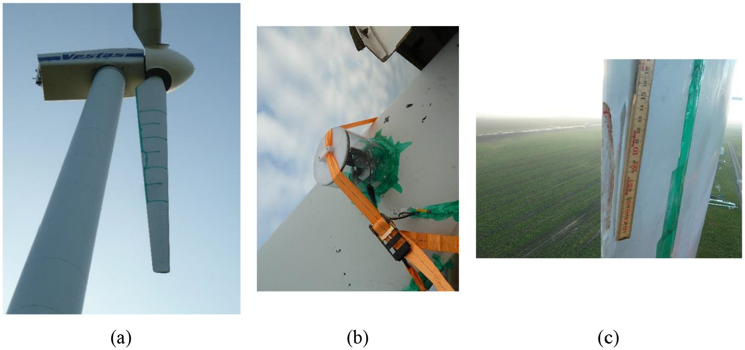
The Vestas V27 wind turbine (a) the turbine, (b) the actuator, and (c) the 15 cm trailing edge damage.

In addition to the excitation caused by a normal operation of the blade, an electromechanical actuator was also used to enhance the amplitude of the acceleration signals, as shown in Figure 1(b). It consists of a coil mounted on a steel base, which was driven by an electrical pulse. This pulse causes the coil to “shoot” a plunger toward the structure, and after the impact, the plunger retracts to its initial position.²⁶ The actuator was mounted on the upwind side of the blade, about 1 m from the root, covered by a waterproof lid, and secured with a strap.

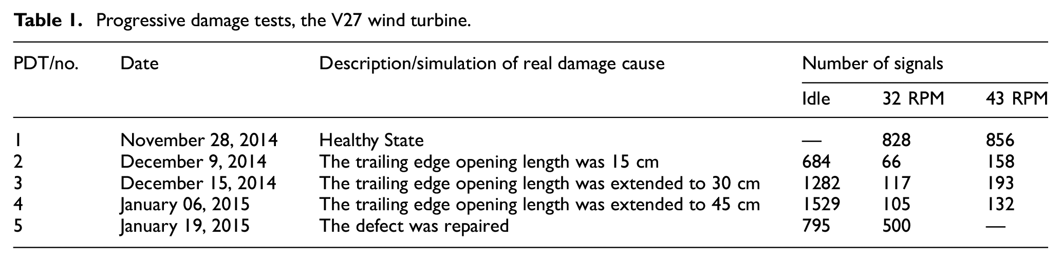
To introduce damage scenarios on the blade, a small defect simulating an adhesive joint failure between skins (trailing edge opening) was introduced in the blade (see Figure 1(c)). The initial length of the defect is 15 cm in the first damage scenario, and it is progressively increased to 30 and 45 cm in the second and the third states, respectively. Several signals were recorded over a 104-day-long testing period, as given in Table 1. The location of the actuator, sensors, and damage locations are shown in Figure 2.

Table 1.

Progressive damage tests, the V27 wind turbine.

PDT/no.	Date	Description/simulation of real damage cause	Number of signals
			Idle	32 RPM	43 RPM
1	November 28, 2014	Healthy State	—	828	856
2	December 9, 2014	The trailing edge opening length was 15 cm	684	66	158
3	December 15, 2014	The trailing edge opening length was extended to 30 cm	1282	117	193
4	January 06, 2015	The trailing edge opening length was extended to 45 cm	1529	105	132
5	January 19, 2015	The defect was repaired	795	500	—

Figure 2.

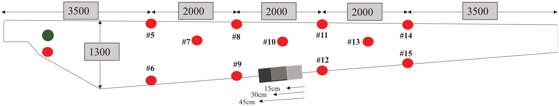
The schematic diagram of the wind turbine blade (not to scale) shows the location of the actuator (green circle), sensors (red circles), and damage locations (grey tone rectangles). The main spar is indicated by dashed lines (dimensions in mm).

According to Tcherniak and Larsen,⁷⁴ the number and placement of accelerometers on each blade were carefully chosen to balance the need for detailed mode shape resolution and the complexity of the data acquisition system. A total of 12 accelerometer channels per blade were used, with 10 monitoring flapwise vibrations (which also capture torsional modes) and 2 edgewise vibrations. The sensitivity of the accelerometers was selected based on numerical simulations using the HAWC-2 software. To ensure accurate and consistent placement across all three blades, the rotor was removed and placed on the ground, using a template and laser distance meter to guarantee uniform positioning. This careful setup ensures reliable data collection for analyzing the blade’s dynamic response under different damage scenarios.

Data acquisition system and wireless data transmission

According to According to Tcherniak and Larsen,^74,75 the data acquisition system, shown in Figure 3, is based on a Brüel & Kjær Type 3660-C setup, comprising a 12-channel input module (Type 3053-B-120) and a 4-channel input/output module (Type 3160-A-042). This system is housed in a waterproof enclosure (60 × 45 × 20 cm, 25 kg), mounted within the spinner, and is powered by a 24 V source supplied through a slip ring from the nacelle. Data transmission is wirelessly facilitated via two Cisco AP-1262 access points, utilizing the 802.11n protocol withmultiple input multiple-output (MIMO) and two spatial streams. One access point is situated in the waterproof box, and the other is located in the nacelle, with omnidirectional antennas on the hub and directional antennas in the nacelle to ensure reliable communication despite potential line-of-sight obstructions. The data acquisition process is managed by Brüel & Kjær’s PULSE LabShop software, which records 10 s of data before and 20 s after each actuator impact, with a 4.5-min pause between cycles, producing 12 actuator hit datasets per hour.⁷⁴

Figure 3.

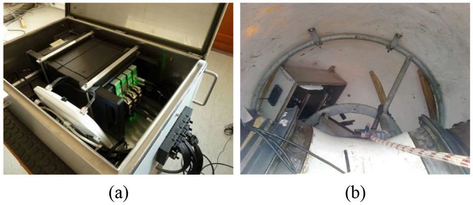
Data acquisition system: (a) waterproof box containing the LAN-XI system with additional modules and (b) waterproof box mounted inside the spinner with cables awaiting connection as explained in detail in Tcherniak and Mølgaard.⁷⁵

Signal preprocessing

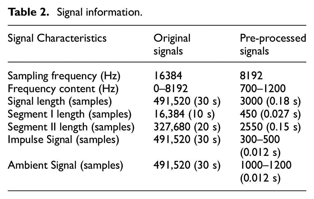
Each recorded signal is trimmed around its periodically incurring peak (corresponding to a hit), with a small, 8000-sample-long, portion retained. This portion is subsequently driven through a 700–1200 Hz bandpass filter, down-sampled by a factor of 2, sample-mean-corrected, and normalized by its sample standard deviation. The resulting vibration response signals are 3000-sample-long and sampled at 8192 Hz.; filter and signal details are provided in Tables 2 and 3, respectively. A typical time-domain signal before and after preprocessing is depicted in Figure 4(a) and (b), respectively. Then, an impulse signal comprising 201 samples between 10.16 and 10.18 s (defined by the red dashed lines), and an ambient signal between 10.2 and 10.22 s (defined by the blue dashed lines) was retained and used for damage feature calculation, as described in Tables 2 and 3.

Table 2.

Signal information.

Signal Characteristics	Originalsignals	Pre-processedsignals
Sampling frequency (Hz)	16384	8192
Frequency content (Hz)	0–8192	700–1200
Signal length (samples)	491,520 (30 s)	3000 (0.18 s)
Segment I length (samples)	16,384 (10 s)	450 (0.027 s)
Segment II length (samples)	327,680 (20 s)	2550 (0.15 s)
Impulse Signal (samples)	491,520 (30 s)	300–500(0.012 s)
Ambient Signal (samples)	491,520 (30 s)	1000–1200(0.012 s)

Table 3.

Bandpass filter parameters.

Elliptic bandpass filter

Bandpass edge: 700 Hz, 1200 Hz; stopband edge: 600 Hz, 1300 Hz; passband ripple:1 Hz; stopband attenuation: 60 dB; sampling frequency: 16384 Hz

Figure 4.

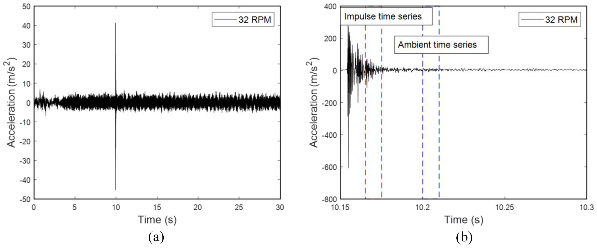
Typical signals: (a) original signal in the time domain and (b) its final (trimmed, bandlimited, and down-sampled signal) counterpart. The dashed rectangle indicates the final trim of the Impulse and Ambient signal.

Damage classification framework with optimized FS

This section presents the supervised damage classification framework. The framework includes five steps: (1) data collection, (2) signal preprocessing, (3) feature estimation, (4) FS, and (5) feature classification (see Figure 5). While the first two steps, covering data collection and signal preprocessing, were previously discussed in section “Experimental setup,” this section now delves into the subsequent stages, exploring feature engineering and model development aspects.

Figure 5.

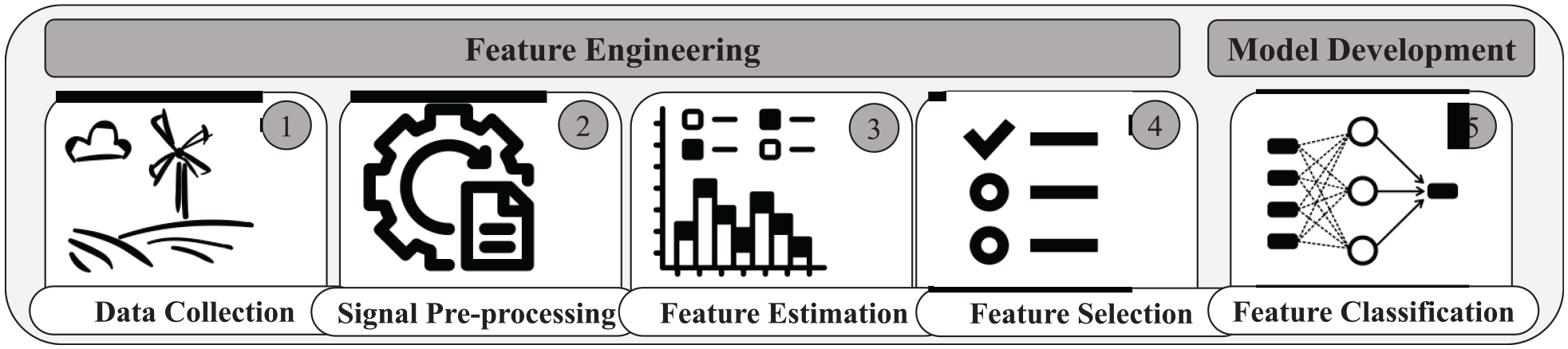
A summary of the optional steps and techniques involved in a data-driven SHM system with ML augmentation.

Feature estimation

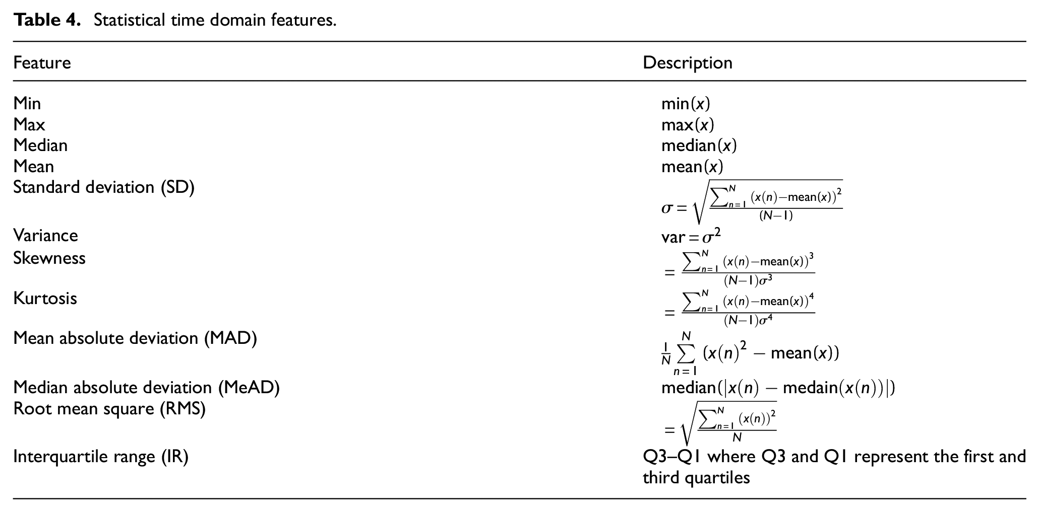
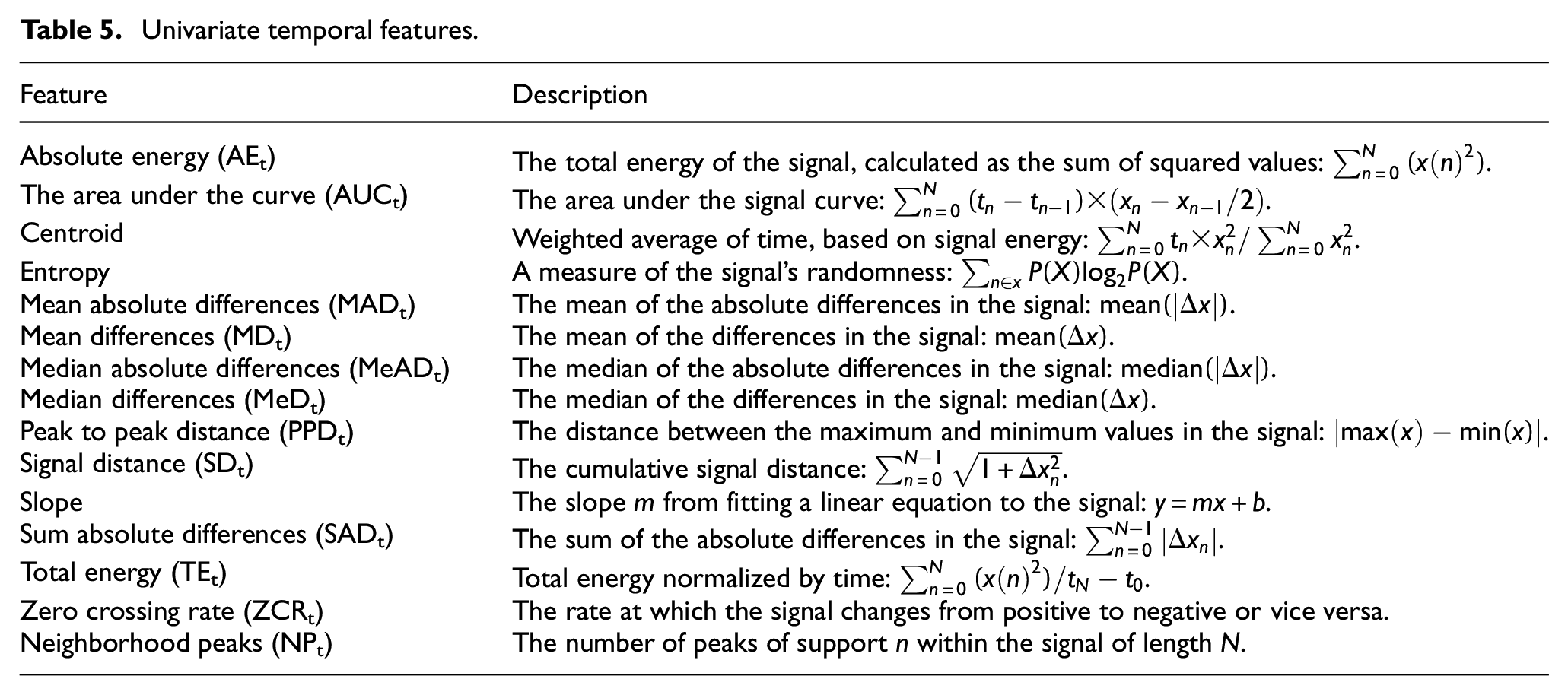
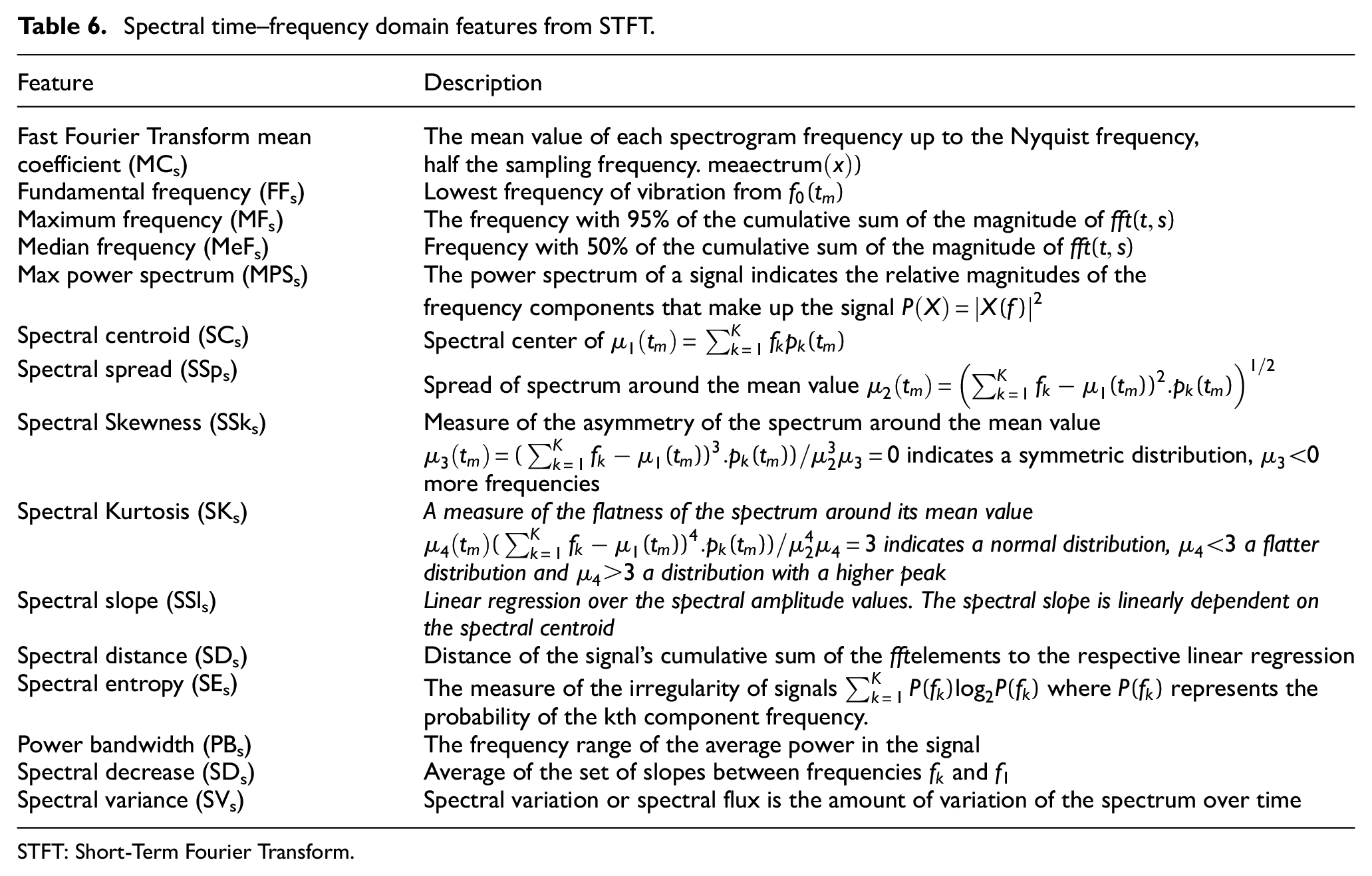
Univariate features are signal processing methods that can be obtained from individual accelerometer recordings within a specific time window. These features summarize the dynamic characteristics of the structure during that period, and changes in them indicate the behavior of the system over time. Although different features may have various sensitivities to damage or be prone to false positives due to environmental and operational factors, evaluating features can improve overall damage detection capability. Three main features are used including (a) statistical, (b) temporal, and (c) spectral ones, as shown in Tables 4 to 6.

Table 4.

Statistical time domain features.

Feature	Description
Min	$\min (x)$
Max	$\max (x)$
Median	$median (x)$
Mean	$mean (x)$
Standard deviation (SD)	$σ = \sqrt{\frac{\sum_{n = 1}^{N} {(x (n) - mean (x))}^{2}}{(N - 1)}}$
Variance	$var = σ^{2}$
Skewness	$= \frac{\sum_{n = 1}^{N} {(x (n) - mean (x))}^{3}}{(N - 1) σ^{3}}$
Kurtosis	$= \frac{\sum_{n = 1}^{N} {(x (n) - mean (x))}^{4}}{(N - 1) σ^{4}}$
Mean absolute deviation (MAD)	$\frac{1}{N} \sum_{n = 1}^{N} (x {(n)}^{2} - mean (x))$
Median absolute deviation (MeAD)	$median (\| x (n) - medain (x (n)) \|)$
Root mean square (RMS)	$= \sqrt{\frac{\sum_{n = 1}^{N} {(x (n))}^{2}}{N}}$
Interquartile range (IR)	Q3–Q1 where Q3 and Q1 represent the first andthird quartiles

Table 5.

Univariate temporal features.

Feature	Description
Absolute energy (AE_t)	The total energy of the signal, calculated as the sum of squared values: $\sum_{n = 0}^{N} (x {(n)}^{2})$ .
The area under the curve (AUC_t)	The area under the signal curve: $\sum_{n = 0}^{N} (t_{n} - t_{n - 1}) \times (x_{n} - x_{n - 1} / 2)$ .
Centroid	Weighted average of time, based on signal energy: $\sum_{n = 0}^{N} t_{n} \times x_{n}^{2} / \sum_{n = 0}^{N} x_{n}^{2}$ .
Entropy	A measure of the signal’s randomness: $\sum_{n \in x} P (X) \log_{2} P (X)$ .
Mean absolute differences (MAD_t)	The mean of the absolute differences in the signal: $mean (\| Δ x \|)$ .
Mean differences (MD_t)	The mean of the differences in the signal: $mean (Δ x)$ .
Median absolute differences (MeAD_t)	The median of the absolute differences in the signal: $median (\| Δ x \|)$ .
Median differences (MeD_t)	The median of the differences in the signal: $median (Δ x)$ .
Peak to peak distance (PPD_t)	The distance between the maximum and minimum values in the signal: $\| max (x) - \min (x) \|$ .
Signal distance (SD_t)	The cumulative signal distance: $\sum_{n = 0}^{N - 1} \sqrt{1 + Δ x_{n}^{2}}$ .
Slope	The slope $m$ from fitting a linear equation to the signal: $y = mx + b$ .
Sum absolute differences (SAD_t)	The sum of the absolute differences in the signal: $\sum_{n = 0}^{N - 1} \| Δ x_{n} \|$ .
Total energy (TE_t)	Total energy normalized by time: $\sum_{n = 0}^{N} (x {(n)}^{2}) / t_{N} - t_{0}$ .
Zero crossing rate (ZCR_t)	The rate at which the signal changes from positive to negative or vice versa.
Neighborhood peaks (NP_t)	The number of peaks of support $n$ within the signal of length N.

Table 6.

Spectral time–frequency domain features from STFT.

Feature	Description
Fast Fourier Transform meancoefficient (MC_s)	The mean value of each spectrogram frequency up to the Nyquist frequency,half the sampling frequency. $meaectrum (x))$
Fundamental frequency (FF_s)	Lowest frequency of vibration from $f_{0} (t_{m})$
Maximum frequency (MF_s)	The frequency with 95% of the cumulative sum of the magnitude of $fft (t, s)$
Median frequency (MeF_s)	Frequency with 50% of the cumulative sum of the magnitude of $fft (t, s)$
Max power spectrum (MPS_s)	The power spectrum of a signal indicates the relative magnitudes of the frequency components that make up the signal $P (X) = {\| X (f) \|}^{2}$
Spectral centroid (SC_s)	Spectral center of $μ_{1} (t_{m}) = \sum_{k = 1}^{K} f_{k} p_{k} (t_{m})$
Spectral spread (SSp_s)	Spread of spectrum around the mean value $μ_{2} (t_{m}) = {(\sum_{k = 1}^{K} f_{k} - μ_{1} (t_{m}))^{2} . p_{k} (t_{m}))}^{1 / 2}$
Spectral Skewness (SSk_s)	Measure of the asymmetry of the spectrum around the mean value $μ_{3} (t_{m}) = (\sum_{k = 1}^{K} f_{k} - μ_{1} (t_{m}))^{3} . p_{k} (t_{m})) / μ_{2}^{3} μ_{3} = 0$ indicates a symmetric distribution, $μ_{3} < 0$ more frequencies
Spectral Kurtosis (SK_s)	A measure of the flatness of the spectrum around its mean value $μ_{4} (t_{m}) (\sum_{k = 1}^{K} f_{k} - μ_{1} (t_{m}))^{4} . p_{k} (t_{m})) / μ_{2}^{4} μ_{4} = 3$ indicates a normal distribution, $μ_{4} < 3$ a flatterdistribution and $μ_{4} > 3$ a distribution with a higher peak
Spectral slope (SSl_s)	Linear regression over the spectral amplitude values. The spectral slope is linearly dependent onthe spectral centroid
Spectral distance (SD_s)	Distance of the signal’s cumulative sum of the $fft$ elements to the respective linear regression
Spectral entropy (SE_s)	The measure of the irregularity of signals $\sum_{k = 1}^{K} P (f_{k}) \log_{2} P (f_{k})$ where $P (f_{k})$ represents the probability of the kth component frequency.
Power bandwidth (PB_s)	The frequency range of the average power in the signal
Spectral decrease (SD_s)	Average of the set of slopes between frequencies $f_{k}$ and $f_{1}$
Spectral variance (SV_s)	Spectral variation or spectral flux is the amount of variation of the spectrum over time

STFT: Short-Term Fourier Transform.

Statistical time domain features are fundamental signal features that summarize signal statistics over a window in the time domain. In the following, the features are typically represented using a formula, where $x$ denotes the acceleration signal vector, $t$ is the corresponding time domain vector, $fs$ is the sampling frequency, $N$ is the length of $x$ , and $P (X)$ represents the state probability.

Temporal features are extracted from the time series and describe signal dynamics over time in the feature extraction window. Equations for the features include $Δ x$ (discrete derivative of the signal vector), with temporal discretization involving integration over the time step ( $Δ t$ ).

Spectral time–frequency features represent the signal change in the frequency domain over time. This analysis uses STFT as the spectral approach to obtain time–frequency domain features. The first set of spectral features is obtained by applying a STFT to the signal window. The STFT is calculated by dividing the signal into small overlapping time windows and calculating the Fourier transform for each window, producing a spectrogram. The discrete STFT is then defined, and the normalized value of the amplitude value of the magnitude of the STFT can be computed.⁷⁶ When the windowed signal input into feature extraction algorithms, it can create spectral leakage, which can be reduced by using a Tukey window with a 12.5% overlap.⁷⁷ Table 6 displays the spectral features that can be obtained from the STFT, which can describe the statistical properties of the signal and the magnitude of the spectrum.

Feature selection

Feature selection has gained significant importance in data analysis, ML, and data mining, especially when dealing with high-dimensional datasets. It is crucial to sift through irrelevant and redundant features by selecting a relevant subset to prevent overfitting and address the problem of high dimensionality. Among the methods used for feature selection, filter methods are particularly valuable because they can be seamlessly integrated with various ML models and significantly reduce computation time. An example of a filter method is the ANOVA F-test, which operates independently of classifiers and evaluates feature relevance before modeling.⁷⁸ The ANOVA algorithm calculates an F statistic for each feature by analyzing the variance explained by that feature with respect to the class variable. A higher F statistic indicates greater differentiation in the mean values of the feature across different classes. For each feature $X_{k}$ , the filter score is defined as Equation (1):

J_{ANOVA} (X_{k}) = \frac{\sum_{i = 1}^{l} n_{i} {({\bar{x}}_{i}^{(k)} - {\bar{x}}_{i}^{(k)})}^{2} / (l - 1)}{\sum_{i = 1}^{l} \sum_{j = 1}^{n_{i}} {({\bar{x}}_{ij}^{(k)} - {\bar{x}}_{i}^{(k)})}^{2} / (n - 1)}

(1)

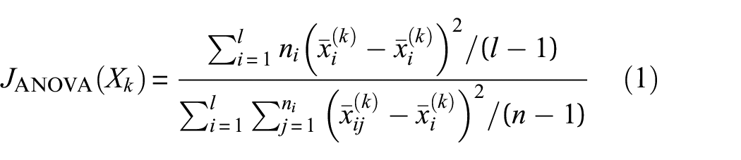
where l denotes the number of classes of Y and $X_{ij}^{(k)}$ , $i \in {1, \dots, n_{i}}$ , denote the observed values of features $X_{k}$ for instances of class $i$ . ${\bar{x}}_{i}^{(k)} = \frac{1}{n} \sum_{j = 1}^{n_{i}} x_{ij}^{(k)}$ is the mean value of $X_{k}$ in class $i$ and ${\bar{x}}^{(k)} = \frac{1}{n} \sum_{i = 1}^{l} \sum_{j = 1}^{n_{i}} x_{ij}^{(k)}$ is the mean value of all instances in the dataset.⁷⁹

To analyze how prediction accuracy varies with the inclusion of different percentiles of ANOVA-ranked features for each classification model, a pipeline is presented for evaluating accuracy variation during a fivefold cross-validation. To maintain data integrity, the ANOVA filter is applied separately to the training data in each fold.

Feature classification

Supervised learning trains an algorithm using labeled data containing input and corresponding target variables. The goal is to build a model that predicts the target variable accurately based on the input variables. Model performance is assessed by comparing its predictions on new data to actual target values. This involves choosing an algorithm, identifying relevant features, and optimizing model parameters for optimal outcomes. The classifiers used are SVM, DT, DA, ET, RF, KNN, and NN classifiers.

SVM is highly effective for problems involving complex and high-dimensional data, such as in SHM. It works by finding the optimal boundary (or hyperplane) that best separates the different classes (e.g., healthy vs. damaged states) in the data. SVM is especially powerful because it maximizes the margin between classes, which help in accurate classification even when the data are not easily separable. The performance of SVM is significantly influenced by selecting the correct kernel function and tuning key parameters.³⁴ DA is a classification method that assumes that data from each class has a different statistical distribution, unlike linear discriminant analysis, which assumes identical variances across classes. DA is more flexible as it does not assume an equal spread between the classes but can be prone to overfitting, especially when there are more features than samples. Regularization techniques are used to optimize DA and avoid overfitting by controlling the complexity of the model.⁶²

RF and ET are powerful ensemble learning methods that build multiple decision trees and combine their predictions to improve the overall accuracy and robustness of a model, especially when dealing with noisy and high-dimensional data like that found in SHM. RF reduces the risk of overfitting by training trees on random subsets of data and averaging their predictions. Similarly, ET methods, such as RF, are particularly effective in SHM applications, where detecting subtle differences between damage states is crucial, as they can capture a wide range of patterns across the data. Both RF and ET models can be optimized by tuning parameters, such as the number of trees and their depth, which helps balance model accuracy and complexity, ultimately preventing overfitting and enhancing the generalization of the model.^59,60 KNN is a simple, intuitive method that classifies a data point by looking at its nearest neighbors in the dataset. The class of the data point is determined by the majority class among its closest neighbors. The key parameter in KNN is the number of neighbors to consider, which must be carefully tuned to avoid overfitting or underfitting. This method performs well when the data have clear local patterns.⁶¹

NNs, particularly multilayer perceptrons (MLPs), are powerful tools for capturing complex, nonlinear relationships in data. Since SHM data often involve intricate interactions between various features, neural networks are well-suited for modeling these relationships. However, neural networks require careful tuning of parameters such as the number of hidden layers, neurons per layer, and the learning rate. Techniques like grid search are often used to optimize these parameters and find the best model setup for accurate predictions.⁶⁵ All information about parameter setting and its values are described on Table 7.

Table 7.

Parameter settings for the comparative algorithms.

Algorithm	Parameter	Value
SVM	Kernel Function Kernel Scale	Radial basis function Automatic kernel scaleselection
DT	Number of Split	50
QDA	Function	Pseudoquadratic
ET	Number of Split Training Method	50 Bagging
RF	Number Tree Function	50 Tree Bagger
KNN	Number of neighbors	5
NN	Hidden layer Max epochs	[10 10 10] 50

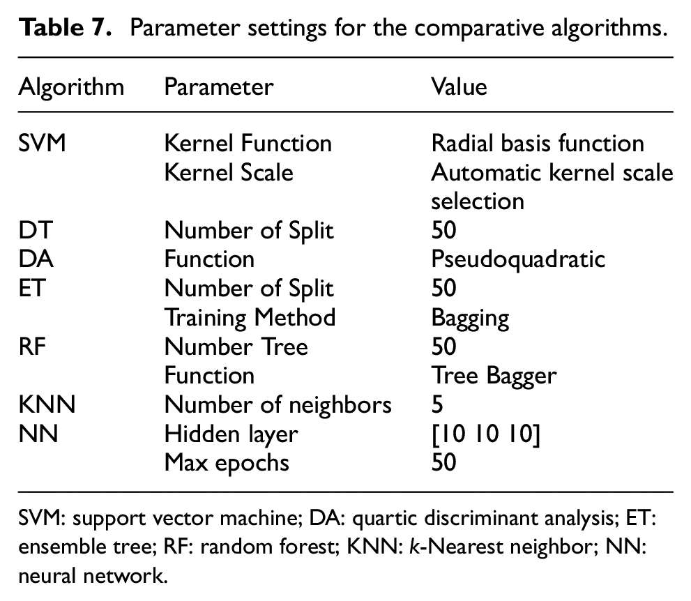
SVM: support vector machine; DA: quartic discriminant analysis; ET: ensemble tree; RF: random forest; KNN: k-Nearest neighbor; NN: neural network.

Stratified k-fold cross-validation is a widely used technique for evaluating classification models, and addressing limited training data. The training set is divided into K nonoverlapping folds, using one fold for validation and the rest for training. Performance metrics are averaged over K iterations, providing a reliable estimate. This approach prevents overfitting, ensures accurate model assessment, and accounts for class imbalances.⁸⁰

Evaluation metrics

In this article, the confusion matrix is used to evaluate the performance of a model by comparing actual and predicted results. In a confusion matrix, the diagonal elements normally represent correct predictions for both normal and abnormal states, while the off-diagonal elements indicate misclassifications. In addition, accuracy can be presented in a confusion matrix using the ratio of the correct predictions to the total number of predictions in the diagonal elements. However, in this article, precision and recall are used to measure the model’s effectiveness, with precision evaluating the performance for each class and recall assessing how well the model identifies the true observations. In an unbalanced dataset with more normal than anomalous data points, accuracy may bias results. Precision (Equation (2)), recall (Equation (3)), F1-score (Equation (4)), and Matthews correlation coefficient (MCC) (Equation (5)) are defined as follows:

Precision = \frac{TP}{TP + FP}

(2)

Recall = \frac{TP}{TP + FN}

(3)

F 1 - score = \frac{2 \times Precision \times Recall}{Precision + Recall}

(4)

MCC = \frac{(TP \times TN - FP \times FN)}{\sqrt{(TP + FP) \times (TP + FN) \times (TN + FP) \times (TN + FN)}}

(5)

where TP, FP, FN, and TN are true positive, false positive, false negative, and true negative ratios in the confusion matrix, respectively.⁸¹ The Receiver Operating Characteristic (ROC) curve shows the sensitivity-specificity trade-off and reveals how well a classifier balances true positives and false negatives. Higher sensitivity at a specific specificity indicates superior performance.⁸²

Results and discussions

In this section, the proposed framework is evaluated using the dataset explained in section “Experimental setup.” The objective is to identify the feature sets that maximize classification prediction performance while minimizing the number of features.

Feature estimation and selection process

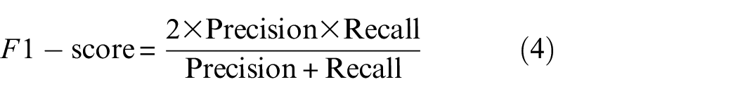
The features are obtained from 12 sensors distributed along the length of the blade, resulting in 504 features in total (12 sensors × 42 features), comprising 12 statistical, 15 temporal, and 15 spectral features. The ANOVA algorithm is employed to select the best features for damage classification. Figure 6 shows a sample of results from the ANOVA F-Test method which ranks the top 15 features. In this figure, the features are shown on the y-axis in the format of “name of the feature”/“Si” in which Si represents the number of the sensors allocated on the blade as shown in Figure 2. For instance, “slope/S9” refers to the feature of “slope” related to S9 which is sensor number 9.

Figure 6.

The 15 top-ranked features obtained from the impulse signals, for (a) the Idle and (b) 32 RPM states.

Classification using impulse signals

In this study, various classification models, including SVM, DT, DA, ET, RF, KNN, and NN, are employed for training, validation, and testing with a comprehensive feature set comprising statistical, temporal, and spectral features separately. A standard fivefold stratified cross-validation scheme is chosen, resulting in an 80%–20% split between training and test data in each fold, respectively, while preserving the original chronological order of data within each class. The performance of these algorithms in the damage detection model is evaluated using multiple metrics outlined in section “Evaluation metrics.” The F1 score is presented for each algorithm in Figure 7. This figure shows the results when spectral feature subsets of all, the top-ranked 150, 100, 70, 50, 30, and 10 features are selected using ANOVA.

Figure 7.

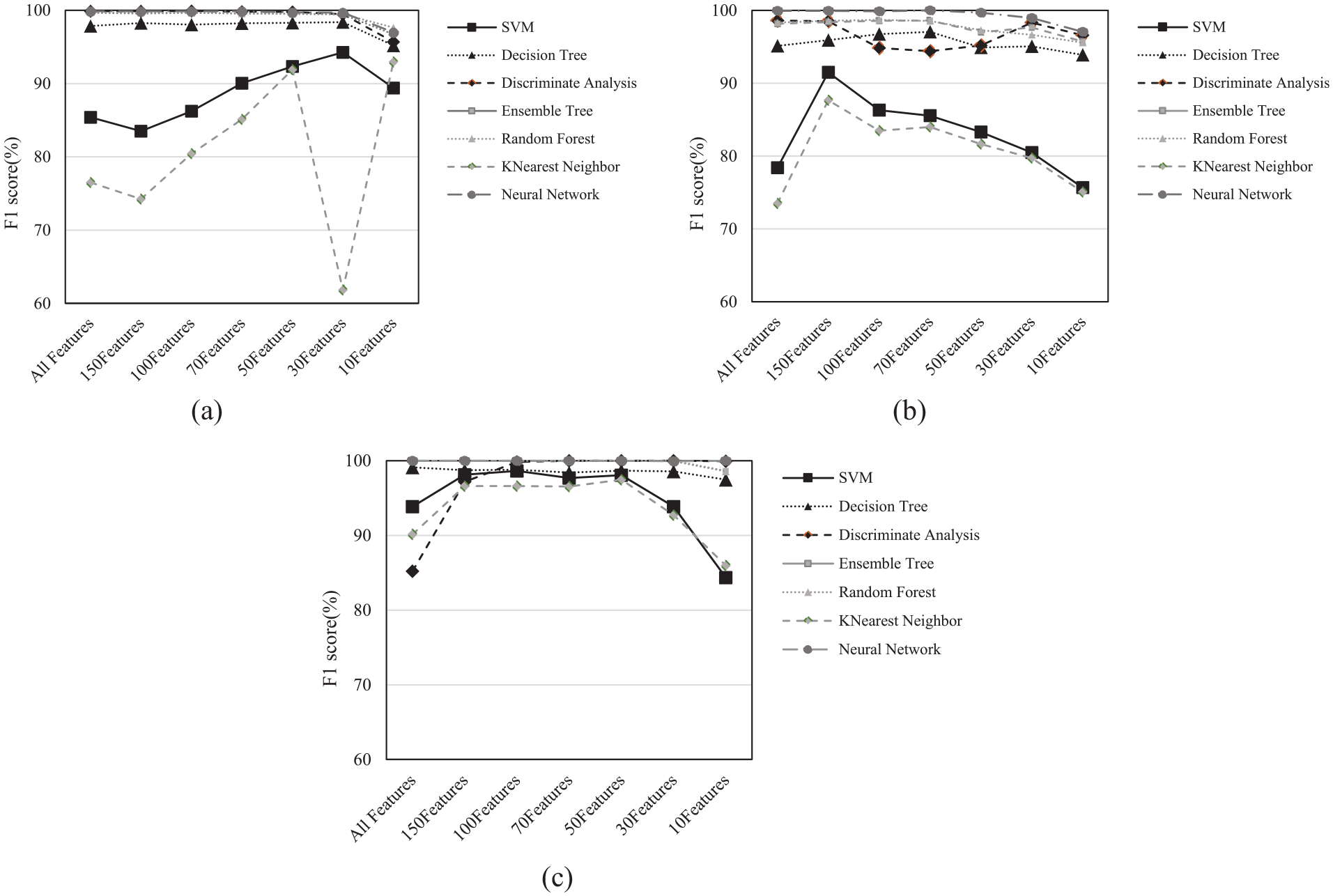
F1 score for spectral features of the impulse signal of the (a) Idle, (b) 32 RPM, and (c) 43 RPM state in different features.

Figure 7 shows that the top-performing classification methods maintain over 95% accuracy in most cases when a minimum of 10, 30, or 50 features are selected. However, the type of classification algorithm plays an important role in the classification accuracy. For example, classification methods such as DT, DA, ET, RF, and NN show reasonably high accuracy often reaching or surpassing 90% accuracy, while SVM and KNN show a poor performance. However, it is worth mentioning that in some cases, NN classifications achieve better accuracy but require significantly more computational time compared to algorithms such as RF. For instance, in the case of 32 RPM, NN classification takes about four times as long as RF, while achieving similar accuracy (96% for NN and 93.94% for RF). In addition, RF offers several advantages such as not requiring pruning, minimal overfitting, tolerance to noise and outliers, stability, and strong generalization. It is also well-suited for parallel computing and performs efficiently with large samples.²⁴

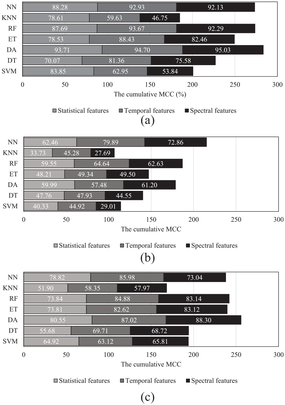
Figure 8 presents cumulative MCC subsets of the top 10 features in statistical, temporal, and spectral categories, used to assess various classifications in different conditions, including Idle, 32, and 43 RPM. It can be seen from this figure that the data from the Idle state provides better overall accuracy compared to the operational conditions. This is most likely due to less measurement noise included in the measured response in the Idle conditions compared to operational conditions. However, when it comes to the operational condition, the results with a higher speed of 43 RPM are significantly better than the ones obtained from 32 RPM. Higher rotational speeds lead to stronger dynamic responses, which result in higher amplitudes in acceleration responses in the relevant frequency ranges. This means that the DSFs can perform better at higher rotational speeds In addition, it can be concluded that, in general, the spectral and temporal features can provide better accuracy compared to statistical features.

Figure 8.

The cumulative MCC of the statistical, temporal, and spectral features by selecting the 10-top ranked features of (a) Idle, (b) 32 RPM, and (c) 43 RPM, Impulse series.

It can be concluded that among various classifier models, excluding SVM and KNN, consistent superiority emerges in wind turbine blade damage detection, achieving notable accuracy, particularly early failure identification through temporal and spectral features. This effectiveness extends to new test data, demonstrating robust generalization and adaptability. Importantly, the RF classifier stands out for its faster runtimes compared to NN, ET, and occasionally SVM models, underscoring computational efficiency. Moreover, data collected during different wind turbine damage states, both Idle and 43 RPM operation, exhibit higher values than at 32 RPM, suggesting the advantage of precision and recall prioritization as datasets expand. The accuracy improves at 43 RPM, compared to 32 RPM. This improvement is further enhanced by the higher-frequency components at 43 RPM, which provides more detailed and distinct signals for better damage detection, as opposed to the lower-frequency components at 32 RPM which offer less resolution and make damage harder to identify.³⁰ This result reaffirms the significance of key features—wind speed at hub height, generator temperature, gearbox temperature, and blade pitch angle—validated by prior research.⁸³

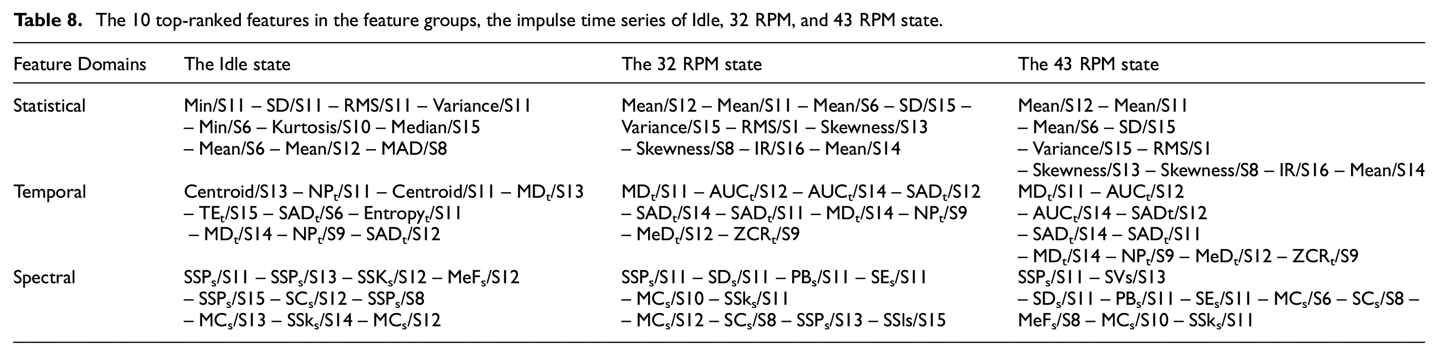
The top 10 ranked features are outlined in Table 8 which provides an insight into the best features. It is evident that most of the top-ranked features are derived from the sensors installed between the damage location and the tip of the blade (e.g., S11–S15). This is also an important finding that shows that the sensors with larger deflections in a composite blade can contain more damage-sensitive information. This finding can also potentially be used for developing a damage localization algorithm in future studies.

Table 8.

The 10 top-ranked features in the feature groups, the impulse time series of Idle, 32 RPM, and 43 RPM state.

Feature Domains	The Idle state	The 32 RPM state	The 43 RPM state
Statistical	Min/S11 – SD/S11 – RMS/S11 – Variance/S11– Min/S6 – Kurtosis/S10 – Median/S15– Mean/S6 – Mean/S12 – MAD/S8	Mean/S12 – Mean/S11 – Mean/S6 – SD/S15 – Variance/S15 – RMS/S1 – Skewness/S13– Skewness/S8 – IR/S16 – Mean/S14	Mean/S12 – Mean/S11– Mean/S6 – SD/S15– Variance/S15 – RMS/S1– Skewness/S13 – Skewness/S8 – IR/S16 – Mean/S14
Temporal	Centroid/S13 – NP_t/S11 – Centroid/S11 – MD_t/S13 – TE_t/S15 – SAD_t/S6 – Entropy_t/S11 – MD_t/S14 – NP_t/S9 – SAD_t/S12	MD_t/S11 – AUC_t/S12 – AUC_t/S14 – SAD_t/S12– SAD_t/S14 – SAD_t/S11 – MD_t/S14 – NP_t/S9 – MeD_t/S12 – ZCR_t/S9	MD_t/S11 – AUC_t/S12– AUC_t/S14 – SADt/S12– SAD_t/S14 – SAD_t/S11– MD_t/S14 – NP_t/S9 – MeD_t/S12 – ZCR_t/S9
Spectral	SSP_s/S11 – SSP_s/S13 – SSK_s/S12 – MeF_s/S12– SSP_s/S15 – SC_s/S12 – SSP_s/S8– MC_s/S13 – SSk_s/S14 – MC_s/S12	SSP_s/S11 – SD_s/S11 – PB_s/S11 – SE_s/S11– MC_s/S10 – SSk_s/S11– MC_s/S12 – SC_s/S8 – SSP_s/S13 – SSls/S15	SSP_s/S11 – SVs/S13– SD_s/S11 – PB_s/S11 – SE_s/S11 – MC_s/S6 – SC_s/S8 –MeF_s/S8 – MC_s/S10 – SSk_s/S11

Classification using ambient time series

In this section, the effectiveness of key components in the presented models is assessed via Idle, 32, and 43 RPM state analysis in the ambient time series, along with sensitivity analysis. Figure 9 illustrates accuracy outcomes when reducing selected features within the spectral-type feature group in various states. Notably, as feature count decreases, F1 score performance experiences a significant drop, particularly in comparison to the impulse time series. It can seen from the results that the classification accuracy of the results from the Idle state is generally higher than the operational states of 32 and 43 RPM. For example, for achieving over 90% accuracy, a minimum of 50–100 features are required for the operational states, while this can be achieved by a minimum of 30 features in the case of the Idle state. In addition, when it comes to the operational states, the results achieved from the signals with higher RPM show a better classification accuracy. This is an important finding which shows that larger speeds could provide more damage-sensitive information.

Figure 9.

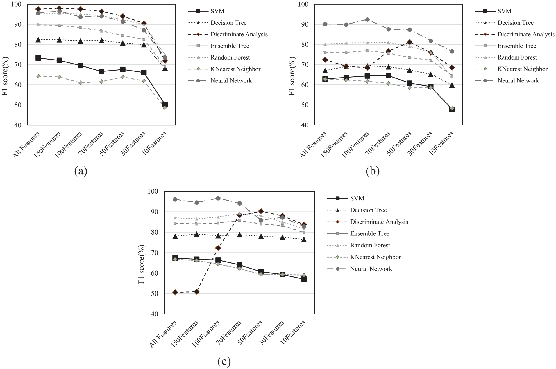
F1 score for spectral features of the ambient signals of the (a) Idle, (b) 32 RPM, and (c) 43 RPM state in different features.

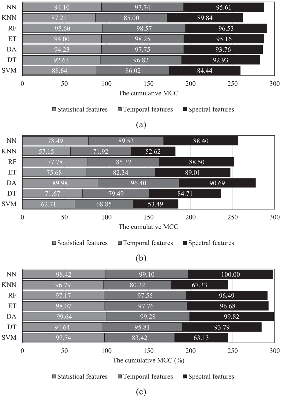
An MCC assessment of the top 50 optimal features is conducted, as depicted in Figure 10. Comparing the results with the impulse case, the MCCs show a relatively lower accuracy in all states. A similar trend as Figure 9 can be observed here. This means that the MCC results from the Idle state (Figure 10(a)) show significantly higher accuracy compared to the ones obtained from the operational states (Figure 10(b) and (c)). For example, some of the classification algorithms such as NN, RF, and DA show the MCC around 289/300, while the maximum cumulative MCC in operational states is around 260/300 corresponding to the DA algorithm obtained from the 43 RPM state. In addition, these results also confirm that the results from a higher RPM in the operational states are better. For example, most feature groups’ cumulative MCC remains below 200 when the signals from 32 RPM are used.

Figure 10.

The cumulative MCC of the statistical, temporal, and spectral features by selecting the 50-top ranked features of (a) Idle state, (b) 32 RPM state, and (c) 43 RPM state, Ambient signal.

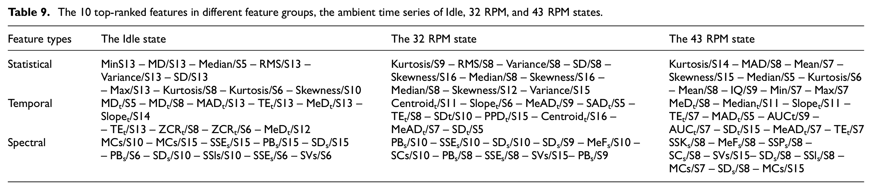
Table 9 lists the top features selected in different scenarios using ambient signals. It shows that the top is mostly selected from the sensors located all along the blade (unlike the results obtained from impulse signals).

Table 9.

The 10 top-ranked features in different feature groups, the ambient time series of Idle, 32 RPM, and 43 RPM states.

Feature types	The Idle state	The 32 RPM state	The 43 RPM state
Statistical	MinS13 – MD/S13 – Median/S5 – RMS/S13 – Variance/S13 – SD/S13– Max/S13 – Kurtosis/S8 – Kurtosis/S6 – Skewness/S10	Kurtosis/S9 – RMS/S8 – Variance/S8 – SD/S8 –Skewness/S16 – Median/S8 – Skewness/S16 –Median/S8 – Skewness/S12 – Variance/S15	Kurtosis/S14 – MAD/S8 – Mean/S7 –Skewness/S15 – Median/S5 – Kurtosis/S6– Mean/S8 – IQ/S9 – Min/S7 – Max/S7
Temporal	MD_t/S5 – MD_t/S8 – MAD_t/S13 – TE_t/S13 – MeD_t/S13 –Slope_t/S14– TE_t/S13 – ZCR_t/S8 – ZCR_t/S6 – MeD_t/S12	Centroid_t/S11 – Slope_t/S6 – MeAD_t/S9 – SAD_t/S5 –TE_t/S8 – SDt/S10 – PPD_t/S15 – Centroid_t/S16 –MeAD_t/S7 – SD_t/S5	MeD_t/S8 – Median_t/S11 – Slope_t/S11 –TE_t/S7 – MAD_t/S5 – AUCt/S9 –AUC_t/S7 – SD_t/S15 – MeAD_t/S7 – TE_t/S7
Spectral	MCs/S10 – MCs/S15 – SSE_s/S15 – PB_s/S15 – SD_s/S15– PB_s/S6 – SD_s/S10 – SSls/S10 – SSE_s/S6 – SVs/S6	PB_s/S10 – SSE_s/S10 – SD_s/S10 – SD_s/S9 – MeF_s/S10 –SCs/S10 – PB_s/S8 – SSE_s/S8 – SVs/S15– PB_s/S9	SSK_s/S8 – MeF_s/S8 – SSP_s/S8 –SC_s/S8 – SVs/S15– SD_s/S8 – SSl_s/S8 –MCs/S7 – SD_s/S8 – MCs/S15

Comparison between the impulse and ambient time series

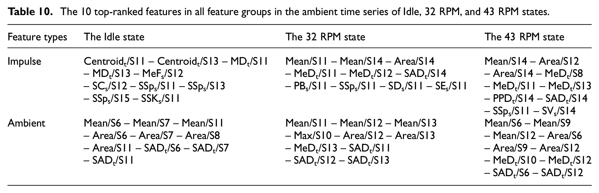
In the proposed methodology, feature extraction and classification play a crucial role in damage detection. These steps are examined across different operational regimes and feature types, including statistical, temporal, and spectral features. Analyzing both impulse and ambient signals with features combined from all domains identifies the highest-ranked features and reveals their associations with specific feature domains and sensor locations. Table 10 displays the top 10 features for each operational state (Idle, 32 RPM, and 43 RPM) and time series type, while Figure 11 further investigates feature sensitivity to damage, showing feature distribution by sensor location and feature domain. Further analysis, reducing feature sets from 50 to 10 across statistical, temporal, and spectral domains presented in Supplemental Tables 1 to 3.

Table 10.

The 10 top-ranked features in all feature groups in the ambient time series of Idle, 32 RPM, and 43 RPM states.

Feature types	The Idle state	The 32 RPM state	The 43 RPM state
Impulse	Centroid_t/S11 – Centroid_t/S13 – MD_t/S11– MD_t/S13 – MeF_s/S12– SC_s/S12 – SSp_s/S11 – SSp_s/S13– SSp_s/S15 – SSK_s/S11	Mean/S11 – Mean/S14 – Area/S14– MeD_t/S11 – MeD_t/S12 – SAD_t/S14– PB_s/S11 – SSp_s/S11 – SD_s/S11 – SE_s/S11	Mean/S14 – Area/S12– Area/S14 – MeD_t/S8– MeD_t/S11 – MeD_t/S13– PPD_t/S14 – SAD_t/S14– SSp_s/S11 – SV_s/S14
Ambient	Mean/S6 – Mean/S7 – Mean/S11– Area/S6 – Area/S7 – Area/S8– Area/S11 – SAD_t/S6 – SAD_t/S7– SAD_t/S11	Mean/S11 – Mean/S12 – Mean/S13– Max/S10 – Area/S12 – Area/S13– MeD_t/S13 – SAD_t/S11 – SAD_t/S12 – SAD_t/S13	Mean/S6 – Mean/S9 – Mean/S12 – Area/S6– Area/S9 – Area/S12– MeD_t/S10 – MeD_t/S12– SAD_t/S6 – SAD_t/S12

Figure 11.

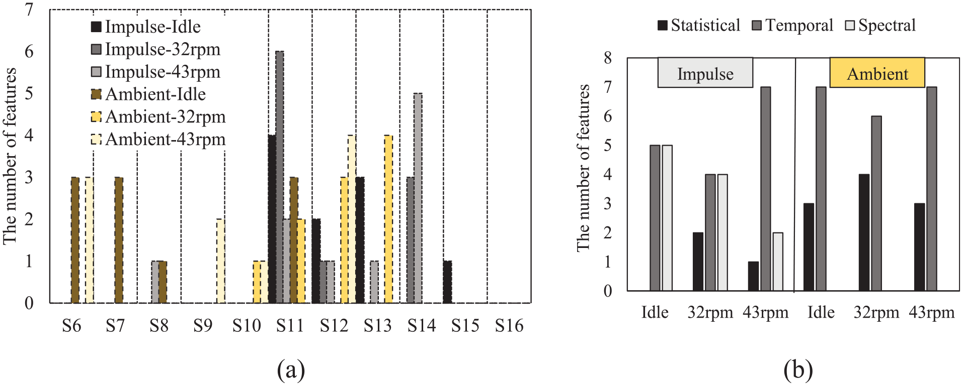
The number of features corresponding to (a) which sensor and (b) which feature groups.

Figure 11 provides insights into the feature distribution relevant to damage detection across different operational regimes. Figure 11(a) reveals that features near sensors 11–14, especially those near the blade tip, are highly sensitive to impulse signals. For example, in the impulse-32 RPM regime (the dark gray box), features from sensors 11, 14, and 12 dominate the rankings, reflecting heightened stress and dynamic motion at the blade tip, which makes it more responsive to structural anomalies. This area is critical in vibration-based damage detection, as shown in related studies.^84,85

Figure 11(b) illustrates feature distribution across statistical, temporal, and spectral domains. For impulse signals, the Idle and 32 RPM states display a balance of temporal and spectral features, but at 43 RPM, temporal features predominate, with seven of the top 10. This trend suggests that spectral features become less effective at higher speeds, likely due to increased vibration frequencies masking damage signals⁴⁷ In ambient signals, statistical and temporal features dominate, while STFT-based spectral features show reduced reliability under nonstationary conditions, where operational fluctuations can obscure damage indicators.⁸⁶ These findings emphasize the importance of selecting features based on the operational context and signal type to optimize damage detection in wind turbine blades.

To provide a clearer comparison of impulse and ambient time series results across operational states, Table 11 presents weighted F1 scores for the top 10 features across all domains. Scores are color-coded from dark to light gray, indicating high accuracy (above 95%) for most classifiers across Idle, 32, and 43 RPM states. Classifiers such as DA, ET, RF, and NN maintain high accuracy even with reduced features, while SVM and KNN show slight drops, particularly in impulse and ambient conditions at 32 and 43 RPM. This suggests that SVM and KNN are more sensitive to feature reduction, consistent with FS literature, which indicates that complex classifiers often perform less robustly with reduced feature sets.⁸⁷

Table 11.

The weighted F1 score of the 10 top-ranked features in the impulse and ambient time series with different regimes and features.

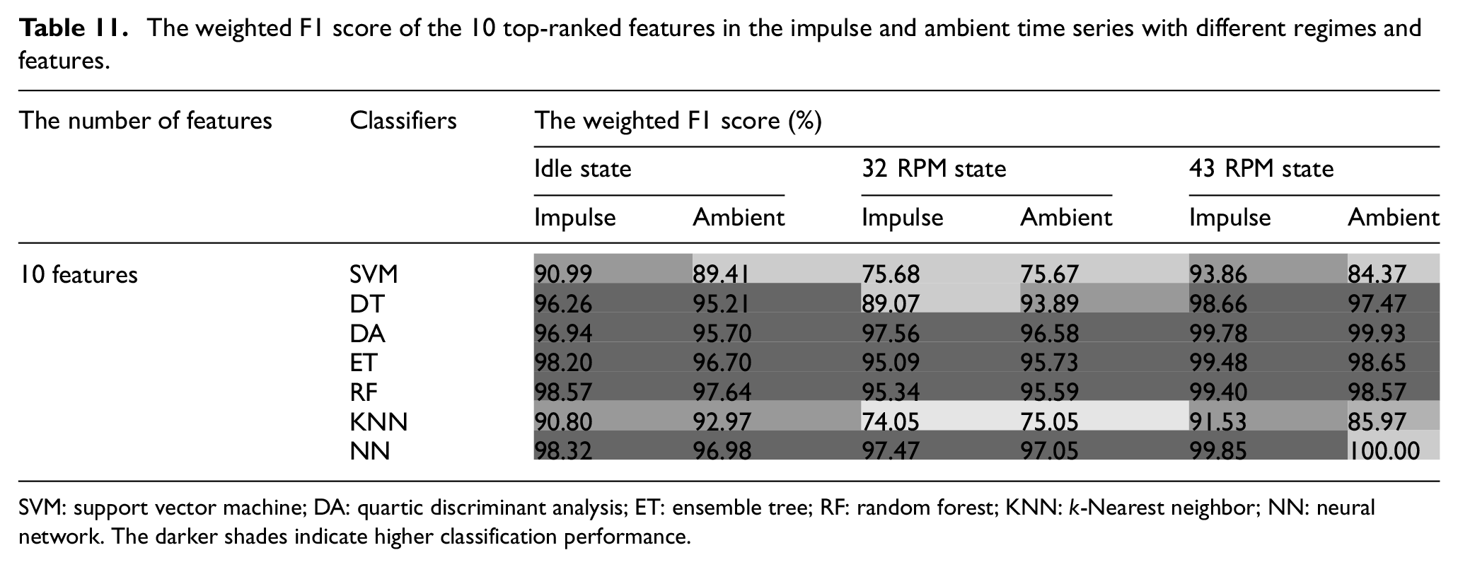
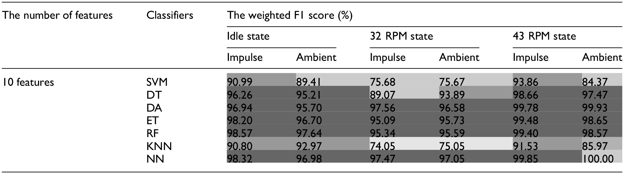
SVM: support vector machine; DA: quartic discriminant analysis; ET: ensemble tree; RF: random forest; KNN: k-Nearest neighbor; NN: neural network. The darker shades indicate higher classification performance.

In the conclusion, this study emphasizes the importance of selecting the right features to improve damage detection in wind turbine blades under varying operational and environmental conditions. Using ANOVA-based filtering on a diverse set of features, the findings show how temporal, spectral, and statistical features perform across different signal types and RPM ranges. ML classifiers like RF and NN prove effective for handling complex, real-world datasets, with multidomain features playing a key role in ensuring reliable classification. By situating these results within the broader SHM literature, the study provides valuable insights into the challenges of real-time monitoring and presents a practical framework for improving damage detection accuracy and efficiency in wind turbines.

Limitations and further investigations

This study identifies several key observations and limitations:

Feature sensitivity and operational variability

Features respond differently to damage depending on the operational state. Impulse signals at lower RPMs allow effective use of temporal, spectral, and statistical features, while higher RPMs reduce spectral feature (STFT) performance due to vibration masking.

For ambient signals, temporal features are more reliable, whereas spectral features like STFT struggle in nonstationary conditions. Tailored FS is essential for accurate results.

Classification and feature reduction

Classifiers such as DA, ET, RF, and NN perform well even with fewer features, but SVM and KNN are more affected by feature reduction, especially at higher RPMs. Impulse signals consistently outperform ambient signals in classification accuracy.

Reducing features from 50 to 10 maintains accuracy for impulse signals but is less effective for ambient signals, emphasizing the need for multidomain features under ambient conditions.

Real-time application challenges

Processing large data volumes and high computational demands pose challenges for real-time implementation. While impulse signals offer robust damage detection across a broad frequency range, the processing requirements can limit practical use.

Opportunities for improvement

Advanced feature techniques: Combining time–frequency analysis with multidomain features could enhance detection, especially for nonstationary ambient signals.

Real-time optimization: Streamlining computational processes for feature extraction and classification is crucial for real-time wind turbine health monitoring.

Conclusion

This study presents a detailed and comparative performance of features for SHM of wind turbine blades in their operational condition, leading to a robust approach toward their choice and implementation. The work addresses the lack of such comparisons, especially with real data and the performance metrics for various ML approaches. This framework for supervised damage classification for operational wind turbine blades, capitalizing on the ANOVA algorithm for FS filtering also creates possibilities for other future algorithms and comparisons in a bespoke manner. Selection of optimal and streamlined set of features to bolster classification efficiency in detecting and differentiating damage states are established. A detailed pool of 12 time-domain, 15 frequency-domain, and 15 time–frequency domain features is considered to capture insights from measured acceleration time-series data and related detection. The work investigates a diverse array of classification methods to delineate distinct damage states, and focuses on a 15 cm damaged state within the 32 RPM regime, providing a detailed and representative case. Prominent classification algorithms, encompassing SVM, DT, DA, ET, RF, KNN, and NN, are enlisted to categorize healthy and damaged states. Notably, in the impulse time series, selecting 10 optimal features yields acceptable accuracy across all classifiers in damage detection. Moreover, addressing the challenge of feature extraction amid uncertain ambient vibration condition, the comparative evaluation of supervised classification utilizing selected features from both impulse and ambient time series emerges. For ambient time series, the number of optimal features increases to 50 to achieve accuracy surpassing 90% across various regimes, underscoring RF, DA, and NN as particularly adept at discerning multiple damage scenarios, which are larger than more typical applications in transport networks and reflective of the complexity of the data, system and processes for wind turbine monitoring. This approach has practical implications for real-time SHM systems, enabling effective maintenance planning and safer turbine operation. Future work could broaden this approach to different turbine models, consider more extensive environmental variables, and explore unsupervised learning methods to further enhance the robustness and adaptability of this framework.

Supplemental Material

sj-docx-1-shm-10.1177_14759217251313815 – Supplemental material for Optimum feature selection for the supervised damage classification of an operating wind turbine blade

Supplemental material, sj-docx-1-shm-10.1177_14759217251313815 for Optimum feature selection for the supervised damage classification of an operating wind turbine blade by Mohadeseh Ashkarkalaei, Ramin Ghiasi, Vikram Pakrashi and Abdollah Malekjafarian in Structural Health Monitoring

Footnotes

Declaration of conflicting interests

The author(s) declared no potential conflicts of interest with respect to the research, authorship, and/or publication of this article.

Funding

The author(s) disclosed receipt of the following financial support for the research, authorship, and/or publication of this article: This work has been funded by the Sustainable Energy Authority of Ireland under the SEAI Research, Development & Demonstration Funding Programme 2021, Grant number 21/RDD/601. The authors would also like to acknowledge Sustainable Energy Authority of Ireland project Remote Wind RDD/613, Twinfarm RDD/604, Science Foundation Ireland Funded NexSys 21/SPP/3756 and the SEMPRE project funded under the National Development Plan (NDP) 2018-2027. The authors gratefully acknowledge the support and data from Dr. Dmitri Tcherniak.

ORCID iDs

Mohadeseh Ashkarkalaei

Ramin Ghiasi

Vikram Pakrashi

Abdollah Malekjafarian

Supplemental material

Supplemental material for this article is available online.

References

Jung

Schindler

Projections of energy yield-and complementarity-driven wind energy expansion scenarios in the European Union. Energy Convers Manage 2022; 269: 116160.

Mishnaevsky

Jr.

Repair of wind turbine blades: review of methods and related computational mechanics problems. Renewable Energy 2019; 140: 828–839.

Marin

Barroso

A and

París

, et al. Study of fatigue damage in wind turbine blades. Eng Fail Anal 2009; 16(2): 656–668.

Arapogianni

Genachte

A-B

Manzanas

Deep water. The next step for offshore wind energy. A report by European Wind Energy Agency, 2013.

Lin

Cevasco

Collu

A methodology to develop reduced-order models to support the operation and maintenance of offshore wind turbines. Appl Energy 2020; 259: 114228.

Qiu

Wang

Zeng

, et al. Automatic visual defects inspection of wind turbine blades via YOLO-based small object detection approach. J Electron Imaging 2019; 28(4): 043023.

Zhang

Jackman

. A feasibility study of wind turbine blade surface crack detection using an optical inspection method. In: 2013 International conference on renewable energy research and applications (ICRERA). 2013. IEEE.

Nagarajan

Rajadurai

JS.

A digital image analysis to evaluate delamination factor for wind turbine composite laminate blade. Compos Part B Eng 2012; 43(8): 3153–3159.

Mao

Wang

, et al. Automatic image detection of multi-type surface defects on wind turbine blades based on cascade deep learning network. Intell Data Anal 2021; 25(2): 463–482.

10.

Chen

Zhou

, et al. Shared excitation based nonlinear ultrasound and vibrothermography testing for CFRP barely visible impact damage inspection. IEEE Trans Ind Inform 2018; 14(12): 5575–5584.

11.

LeBlanc

Niezrecki

Avitabile

, et al. Damage detection and full surface characterization of a wind turbine blade using three-dimensional digital image correlation. Struct Health Monit 2013; 12(5–6): 430–439.

12.

Amenabar

Mendikute

López-Arraiza

, et al. Comparison and analysis of non-destructive testing techniques suitable for delamination inspection in wind turbine blades. Compos Part B Eng 2011; 42(5): 1298–1305.

13.

Márquez

FPG

Chacón

AMP

. A review of non-destructive testing on wind turbines blades. Renewable Energy 2020; 161: 998–1010.

14.

Ashkar

Toufigh

Ghaemian

, et al. Application of ultrasonic models for investigating the properties of the interface between roller compacted concrete (RCC) layers. NDT E Int 2021; 124: 102516.

15.

Civera

Surace

Non-destructive techniques for the condition and structural health monitoring of wind turbines: a literature review of the last 20 years. Sensors 2022; 22(4): 1627.

16.

Sierra-Pérez

Torres-Arredondo

Güemes

Damage and nonlinearities detection in wind turbine blades based on strain field pattern recognition. FBGs, OBR and strain gauges comparison. Composite Struct 2016; 135: 156–166.

17.

Farrar

Worden

Structural health monitoring: a machine learning perspective. Chichester, UK: John Wiley & Sons, 2012.

18.

Lotfi

Kargar

Gharehbaghi

, et al. A data-driven robust optimization for multi-objective renewable energy location by considering risk. Env Develop Sustainability. Epub ahead of print 6 June 2022. DOI: 10.1007/s10668-022-02448-7.

19.

Limongelli

Manoach

Quqa

, et al. Vibration response-based damage detection. Struct Health Monit Damage Detection Syst Aerospace 2021; 133–175.

20.

Azam

Mariani

Online damage detection in structural systems via dynamic inverse analysis: a recursive Bayesian approach. Eng Struct 2018; 159: 28–45.

21.

Catbas

Malekzadeh

A machine learning-based algorithm for processing massive data collected from the mechanical components of movable bridges. Autom Constr 2016; 72: 269–278.

22.

Ghiasi

Malekjafarian

Feature subset selection in structural health monitoring data using an advanced binary slime mould algorithm. J Struct Integrity Maint 2023; 8(4): 209–225.

23.

Hoell

Omenzetter

Sequential projection pursuit for optimised vibration-based damage detection in an experimental wind turbine blade. Smart Mater Struct 2018; 27(2): 025007.

24.

Zhang

Liu

Wang

, et al. Ice detection model of wind turbine blades based on random forest classifier. Energies 2018; 11(10): 2548.

25.

Hoell

Omenzetter

Optimal selection of autoregressive model coefficients for early damage detectability with an application to wind turbine blades. Mech Syst Signal Process 2016; 70: 557–577.

26.

Tcherniak

Mølgaard

LL.

Active vibration-based structural health monitoring system for wind turbine blade: demonstration on an operating Vestas V27 wind turbine. Struct Health Monit 2017; 16(5): 536–550.

27.

García Cava

Avendaño-Valencia

Movsessian

, et al. On explicit and implicit procedures to mitigate environmental and operational variabilities in data-driven structural health monitoring. Struct Health Monit Based Data Sci Techniques 2022: 309–330.

28.

Vamvoudakis-Stefanou

Sakellariou

Fassois

SD.

Vibration-based damage detection for a population of nominally identical structures: unsupervised Multiple Model (MM) statistical time series type methods. Mech Syst Signal Process 2018; 111: 149–171.

29.

Spiridonakos

Chatzi

EN.

Metamodeling of dynamic nonlinear structural systems through polynomial chaos NARX models. Comput Struct 2015; 157: 99–113.

30.

Avendano-Valencia

Chatzi

Tcherniak

Gaussian process models for mitigation of operational variability in the structural health monitoring of wind turbines. Mech Syst Signal Process 2020; 142: 106686.

31.

Qadri

Avendaño-Valencia

Hooghoudt

, et al. Removal of environmental and operational effects in damage detection: a comparative study with an operating wind turbine. Struct Health Monit 2020; 20: 8–10.

32.

Panagiotopoulos

Dmitri

Spilios

FD.

Damage detection on the blade of an operating wind turbine via a single vibration sensor and statistical time series methods: exploring the performance limits of robust methods. Struct Health Monit 2023; 22(1): 433–448.

33.

García

Tcherniak

An experimental study on the data-driven structural health monitoring of large wind turbine blades using a single accelerometer and actuator. Mech Syst Signal Process 2019; 127: 102–119.

34.

Santos

Figueiredo

Silva

MFM

, et al. Machine learning algorithms for damage detection: Kernel-based approaches. J Sound Vibr 2016; 363: 584–599.

35.

Maia

JMM

Silva

Almas

EAM

, et al. Damage detection in structures: from mode shape to frequency response function methods. Mech Syst Signal Process 2003; 17(3): 489–498.

36.

Amezquita-Sanchez

Adeli

Signal processing techniques for vibration-based health monitoring of smart structures. Arch Comput Methods Eng 2016; 23: 1–15.

37.

Khazaee

Banakar

Ghobadian

, et al. Fault detection of engine timing belt based on vibration signals using data-mining techniques and a novel data fusion procedure. Struct Health Monit 2016; 15(5): 583–598.

38.

Inturi

Balaji

Gyanam

, et al. An integrated condition monitoring scheme for health state identification of a multi-stage gearbox through Hurst exponent estimates. Struct Health Monit 2023; 22(1): 730–745.

39.

Jiang

L-l

Yin

H-k

X-j

, et al. Fault diagnosis of rotating machinery based on multisensor information fusion using SVM and time-domain features. Shock Vibr 2014, 2014; 4–8.

40.

Ali

Saidi

Harrath

, et al. Online automatic diagnosis of wind turbine bearings progressive degradations under real experimental conditions based on unsupervised machine learning. Appl Acoust 2018; 132: 167–181.

41.

Lei

Lin

, et al. A review on empirical mode decomposition in fault diagnosis of rotating machinery. Mech Syst Signal Process 201335(1–2): 108–126.

42.

Prieto

Cirrincione

Garcia Espinosa

, et al. Bearing fault detection by a novel condition-monitoring scheme based on statistical-time features and neural networks. IEEE Trans Ind Electronics 2012; 60(8): 3398–3407.

43.

Moosavian

Ahmadi

Sakhaei

, et al. Support vector machine and K-nearest neighbour for unbalanced fault detection. J Quality Maintenance Eng 2014; 20(1): 65–75.

44.

Javed

Gouriveau

Zerhouni

, et al. Enabling health monitoring approach based on vibration data for accurate prognostics. IEEE Trans Ind Electron 2014; 62(1): 647–656.

45.

Liao

Wang

Yang

, et al. Binary particle swarm optimization selected time-frequency features for partial discharge signal classification. Int Rev Electrical ENG-IREE 2012; 7(5): 5905–5917.

46.

Bouzida

Touhami

Ibtiouen

, et al. Fault diagnosis in industrial induction machines through discrete wavelet transform. IEEE Trans Ind Electronics 2010; 58(9): 4385–4395.

47.

Qiao

. A survey on wind turbine condition monitoring and fault diagnosis—Part I: components and subsystems. IEEE Trans Ind Electron 2015; 62(10): 6536–6545.

48.

Buckley

Ghosh

Pakrashi

A feature extraction & selection benchmark for structural health monitoring. Struct Health Monit 2023; 22(3): 2082–2127.

49.

Wang

Zhang

, et al. An improved feature selection method based on random forest algorithm for wind turbine condition monitoring. Sensors 2021; 21(16): 5654.

50.

Al-Dabbagh

Neri

Idris

, et al. Algorithmic design issues in adaptive differential evolution schemes: review and taxonomy. Swarm Evol Comput 2018; 43: 284–311.

51.

Dhibi

Mansouri

Hajji

, et al. A novel hybrid methodology for fault diagnosis of wind energy conversion systems. Energy Rep 2023; 9: 5362–5371.

52.

Jiang

Liao

, et al. Probabilistic prognosis of wind turbine faults with feature selection and confidence calibration. IEEE Trans Sustainable Energy 2024; 15: 52–67.

53.

Ruiz

Mujica

Alférez

, et al. Wind turbine fault detection and classification by means of image texture analysis. Mech Syst Signal Process 2018; 107: 149–167.

54.

Dong

Zhang

, et al. Intelligent fault diagnosis of wind turbine gearboxes based on refined generalized multi-scale state joint entropy and robust spectral feature selection. Nonlinear Dyn 2022; 107(3): 2485–2517.

55.

Amiriebrahimabadi

Mansouri

A comprehensive survey of feature selection techniques based on whale optimization algorithm. Multimedia Tools Appl 2024; 83(16): 47775–47846.

56.

Khaire

Dhanalakshmi

. Stability of feature selection algorithm: A review. J King Saud Univ - Comput Inf Sci 2019; 31(4): 504–518.

57.

Bommert

Sun

Bischl

, et al. Benchmark for filter methods for feature selection in high-dimensional classification data. Comput Stat Data Anal 2020; 143: 106839.

58.

Ogaili

AAF

Jaber

Hamzah

MN.

Statistically optimal vibration feature selection for fault diagnosis in wind turbine blade. Int J Renew Energy Res 2023; 13(3): 1082–1092.

59.

Zhang

Wang

, et al. Machine learning-based real-time visible fatigue crack growth detection. Digital Commun Netw 2021; 7(4): 551–558.

60.

Kiani

Camp

Pezeshk

On the application of machine learning techniques to derive seismic fragility curves. Comput Struct 2019; 218: 108–122.

61.

Mucchielli

Bhowmik

Ghosh

, et al. Real-time accurate detection of wind turbine downtime-an Irish perspective. Renewable Energy 2021; 179: 1969–1989.

62.

Mbo’o

Hameyer

. Fault diagnosis of bearing damage by means of the linear discriminant analysis of stator current features from the frequency selection. IEEE Trans Industry Appl 2016; 52(5): 3861–3868.

63.

Jiménez

Muñoz

CQZ

Márquez

FPG

. Dirt and mud detection and diagnosis on a wind turbine blade employing guided waves and supervised learning classifiers. Reliab Eng Syst Saf 2019; 184: 2–12.

64.

Jiménez

Pedro García Márquez

Borja Moraleda

, et al. Linear and nonlinear features and machine learning for wind turbine blade ice detection and diagnosis. Renewable Energy 2019; 132: 1034–1048.

65.

Marugán

Chacón

AMP

Márquez

FPG

. Reliability analysis of detecting false alarms that employ neural networks: a real case study on wind turbines. Reliab Eng Syst Saf 2019; 191: 106574.

66.

Ogaili

AAF

Hamzah

Jaber

AA.

Enhanced fault detection of wind turbine using extreme gradient boosting technique based on nonstationary vibration analysis. J Fail Anal Prev 2024; 24(2): 877–895.

67.

Kaewniam

Cao

Faisal Alkayem

, et al. Recent advances in damage detection of wind turbine blades: a state-of-the-art review. Renewable Sustainable Energy Rev 2022; 167: 112723.

68.

Regan

Canturk

Slavkovsky

, et al. Wind turbine blade damage detection using various machine learning algorithms. In: International design engineering technical conferences and computers and information in engineering conference, 2016. American Society of Mechanical Engineers.

69.

Farhan Ogaili

Mohammed

Jaber

, et al. Automated wind turbines gearbox condition monitoring: a comparative study of machine learning techniques based on vibration analysis. FME Trans 2024; 52(3): 471–485.

70.

Sbarufatti

Optimization of an artificial neural network for fatigue damage identification using analysis of variance. Struct Control Health Monit 2017; 24(9): e1964.

71.

Suresh

Naidu

Mahalanobis-ANOVA criterion for optimum feature subset selection in multi-class planetary gear fault diagnosis. J Vibr Control 2022; 28(21–22): 3257–3268.

72.

Ritto

Rochinha

Digital twin, physics-based model, and machine learning applied to damage detection in structures. Mech Syst Signal Process 2021; 155: 107614.

73.

Luleci

Catbas

Avci

CycleGAN for undamaged-to-damaged domain translation for structural health monitoring and damage detection. Mech Syst Signal Process 2023; 197: 110370.

74.

Tcherniak

Larsen

. Application of OMA to an operating wind turbine: now including vibration data from the blades. In: 5th International operational modal analysis conference, 2013.

75.

Tcherniak

Mølgaard

. Active vibration-based SHM system: demonstration on an operating Vestas V27 wind turbine. In: Proceedings of the 8th European workshop on structural health monitoring (EWSHM 2016), NDT. net., 2016.

76.

Alobaydi

Bakarman

Obeidat

The impact of urban form configuration on the urban heat island: the case study of Baghdad, Iraq. Proc Eng 2016; 145: 820–827.

77.

Oppenheim

AV.

Discrete-time signal processing. New Delhi, India: Pearson Education India, 1999.

78.

Cai

Jiawei

Shulin

, et al. Feature selection in machine learning: a new perspective. Neurocomputing 2018; 300: 70–79.

79.

Rasch

Kubinger

Yanagida

Statistics in psychology using R and SPSS. Hoboken, NJ: John Wiley & Sons, 2011.

80.

Hastie

Tibshirani

Friedman

The elements of statistical learnin. New York, NY: Springer Nature, 2009, p. 33.

81.

Caruana

Niculescu-Mizil

Data mining in metric space: an empirical analysis of supervised learning performance criteria. In: Proceedings of the tenth ACM SIGKDD international conference on Knowledge discovery and data mining, 2004.

82.

Provost

Fawcett

Robust classification for imprecise environments. Mach Learn 2001; 42: 203–231.

83.

Kisvari

Lin

Liu

Wind power forecasting–a data-driven method along with gated recurrent neural network. Renewable Energy 2021; 163: 1895–1909.

84.

Wang

Xue

, et al. Review of the typical damage and damage-detection methods of large wind turbine blades. Energies 2022; 15(15): 5672.

85.

Wang

Liang

Xiang

Damage detection method for wind turbine blades based on dynamics analysis and mode shape difference curvature information. Mech Syst Signal Process 2014; 48(1–2): 351–367.

86.

Feng

Study of structural optimization design on a certain vehicle body-in-white based on static performance and modal analysis. Mech Syst Signal Process 2020; 135: 106405.

87.

Toh

Park

Review of vibration-based structural health monitoring using deep learning. Appl Sci 2020; 10(5): 1680.

Supplementary Material

Please find the following supplemental material available below.

For Open Access articles published under a Creative Commons License, all supplemental material carries the same license as the article it is associated with.

For non-Open Access articles published, all supplemental material carries a non-exclusive license, and permission requests for re-use of supplemental material or any part of supplemental material shall be sent directly to the copyright owner as specified in the copyright notice associated with the article.

0.00 MB

0.10 MB