Sage Journals: Discover world-class research

Abstract

Understanding and predicting damage progression within thin plain-woven carbon fiber-reinforced polymer (CFRP) components is an essential issue for scheduling maintenance intervals and structural inspections and typically requires extensive test series. However, uncertainties always remain and result in conservative design and unnecessary downtimes due to the repeated inspections of a healthy structure. Structural health monitoring (SHM) can be used to reduce these uncertainties, as it allows one to evaluate the condition of a mechanical structure during operation. Numerous SHM methods have been developed, which achieve different levels of damage identification but are often investigated at small coupons with nonrealistic structural damages and loading conditions on both structure and sensor. The present research investigates electrical impedance tomography (EIT) featuring an elastoresistive thin-film sensor to evaluate damage that propagates from a circular hole in a large plate under cyclic tensile–tensile multiblock loading. Applied fatigue loads were increased multiple times up to a total number of two million cycles. During the loading, damage initiated at the hole and continuously propagated into the plate. Repeated EIT evaluations of the applied sensor and validating evaluations by means of digital image correlation clearly revealed the robustness of the hardware and the potential of the SHM method for damage evaluation of plain-woven CFRP components.

Keywords

Electrical impedance tomography CFRP plate with circular hole tension–tension multiblock loading fatigue damage evaluation structural health monitoring damage initiation and propagation

Introduction

Carbon fiber-reinforced polymers (CFRPs) have become an established part of aviation and space industry. Their advantages over metallic materials, particularly in terms of fatigue behavior, cause them to be frequently preferred in recent developments. However, in contrast to metallic materials, fiber-reinforced composites exhibit very complex failure behavior, involving a wide range of damage modes that are dependent on a large number of factors.^1–4

In aerospace, safety is of highest importance. As a consequence, components made from fiber-reinforced composites are often designed with a higher material input than necessary, to include unknown design variables and unforeseen damage mechanisms. This more conservative layout results in more fail-safe components, but is in conflict with traditional lightweight design concepts, as the increased use of material adds additional weight.⁵ This additional material input increases the fuel consumption or decreases the payload.^6,7 As stated by Flower and Soutis,⁸ a reduction of 1% mass could save nearly 3000 l of fuel per year (analyzed for single aisle aircrafts).

Especially in commercial aviation, very high standards for safety and reliability are established, which have to be warranted and guaranteed throughout the service life of an aircraft. For this purpose, the manufacturers specify appropriate maintenance and service schedules, which have to be fulfilled by the operators. These rules also specify relevant inspection methods as well as the location for these inspections. In the case of CFRPs, ultrasonic testing is a well-established and commonly used method for a more in-depth inspection for potential damage locations. However, ultrasonic testing is time-consuming, and thus, the aircrafts experience long and often unnecessary downtimes.^2,9–11

A comparatively novel and widely discussed approach to reduce these downtimes is structural health monitoring (SHM), which monitors the condition of a structural component continuously while an aircraft remains in operational service.^2,11–14 Numerous SHM methods have been developed so far and can be classified into methods that actively excite a structural response or methods that use other sources of excitation, like, for example, mechanical loading. Different methods use, for example, ultrasonic wave propagation or mechanical strains, for damage evaluation.^14–21 Another method is the electrical impedance tomography (EIT)-based reconstruction of the spatial conductivity of an area of interest. This method may be of particular interest for large thin-walled and shell-shaped components, as it uses the mechanical structure itself (if conductive in the right magnitude, e.g., CFRP^22,23) or a thin conductive coating applied onto the structure as a sensor. However, to overcome the challenges associated with direct contacting CFRP laminates and the underlying anisotropic electrical behavior, a conductive coating used as thin-film sensor is often preferred. These thin-film sensors are equipped with electrodes that are placed at their boundaries. The EIT method evaluates the sensor’s spatial conductivity by the electrical potential at the boundary electrodes due to systematic excitation by a defined current pattern. Thus, EIT featuring thin-film sensors can be used to evaluate damages^22,24–26 that change the conductivity of the covering thin film.

Besides these damages that result in very large conductivity drops, recent investigations demonstrated that EIT can also be used to approximate mechanical strains. Tallman et al.²⁷ performed an inverse determination of strains. They applied an analytical piezoresistivity model with which the displacement field and the strains were derived, while the difference between experimentally determined conductivity and the conductivity of the analytical piezoresistivity model was minimized. A similar investigation was carried out by Loh et al.,²⁸ where carbon-nanotube-based sensing skins applied on metallic specimens were utilized to identify spatial strain and impact damage. Another research was conducted by Hassan and Tallman,²⁹ where a generic algorithm and EIT analysis was used to evaluate conductivity changes induced by stress concentrations. The samples used in their research were weakened by a circular hole and subjected to static tensile loads. Validation through digital image correlation (DIC) and numerical simulations demonstrated the accuracy of this proposed model. However, previous research has typically used small specimens and has not investigated their sensor networks or evaluation methods under realistic operational loading conditions, nor for the corresponding damaging behavior.

The present paper investigates the potential of the EIT method featuring conductive thin-film sensors for damage initiation and propagation in CFRP components under fatigue loading. Therefore, a thin-walled plate-shaped plain-woven CFRP specimen with a centrally placed circular hole is considered, and damage induced and propagated by sinusoidal tension–tension loading is examined. During experimental testing, load amplitude adjustments are done to investigate the effect on the damage propagation, as well as on the applied thin-film sensor and the EIT damage evaluation results. Accompanying three-dimensional (3D)-DIC evaluations of the plate surface provide validation for the EIT results. The novelty of this investigation lies on the operational loading conditions and the consequently required compensation of fatigue loading induced changes to the sensor (e.g., “Set-In” effect³⁰ and potential environmental influences). On the basis of the EIT measurements collected throughout the fatigue loading, two damage evaluation approaches are proposed, with which changes to the sensor can be compensated.

The article is structured as follows. First, the preparation of the specimen, the experimental procedure, and the damage evaluation approaches (3D-DIC and EIT) are described. The damage evaluation results by the 3D-DIC and the EIT reconstructions are presented afterward. Finally, the results are discussed and conclusions are made.

Material and methods

The manufacturing process of the specimen along with the experimental setup and procedure for damage evaluation are described in this section.

Specimen

The experimental investigations are performed on the plate-shaped specimen containing a circular hole in its center presented in Figure 1. Therefore, four plain-woven CFRP plies were stacked [45f/0f]_s, vacuum bagged and cured in an autoclave at 120°C and 0.9 MPa to produce a composite blank with a thickness of 0.816 mm. The individual plies contain 3k-T650 fibers and a Solvay CYCOM^®970 resin matrix (Solvay, Brussels, Belgium), with a fiber volume fraction of 0.6. The final specimen geometry and the hole were cut by water jet cutting.

Figure 1.

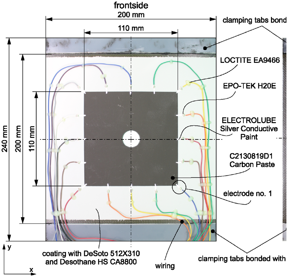
Geometry and dimensions of the plate with hole, location of the GFRP tabs, thin-film sensor with electrodes and cabling, and speckle pattern for 3D-DIC evaluation.

To obtain the configuration, as depicted in Figure 1, the areas that are equipped with the clamping tabs are temporarily taped off and the frontside of the specimen is coated. This coating process, which comprises two steps, begins with the application of a two-component DeSoto^®512X310 Epoxy Primer (PPG Aerospace, Pittsburgh, PA, US). After drying, a layer of a three-component Desothane^® HS CA8800 Topcoat (PPG Aerospace, Pittsburgh, PA, US) is applied. On average, the thickness of the coating is 140 μm.

Once the frontside of the specimen is prepared, the SunChemical^® C2130819D1 Carbon Paste (SunChemical, Parsippany, NJ, US) is deposited on it by screen printing to generate the used elastoresistive thin-film sensor. For this deposition, an aluminum frame with a fine screen (mesh 120 T) is placed on the specimen and the SunChemical^® C2130819D1 Carbon Paste is applied with a silicone squeegee by a single, quick swipe. By masking the screen beforehand, the sensor size and shape is specified. Measurements on an identical specimen provided a mean sensor thickness of 7.35 μm. SunChemical C2130819D1 Carbon Paste has been used by the authors in a previous study, where it was successfully used as EIT sensor material on a high-cycle loaded aluminum specimen.³¹ In addition, the carbon paste was selected due to the fact that sensors with homogeneous conductivity can be realized by screen printing. This allows the fabrication of thin-film sensors with a uniform conductivity distribution. Moreover, further potential influences of inhomogeneous conductivity are excluded through the use of differential EIT.

In a subsequent preparation step, glass fiber-reinforced plastic (GFRP) clamping tabs are bonded in place with 3M^™ Scotch-Weld^™ DP490 (3M, Vienna, Austria), and the backside of the specimen is prepared. On the backside, a white primer is applied, on which small black dots are sprayed by airbrush to create a speckle pattern for the 3D-DIC evaluation. The layer thickness of the applied primer is about 200 μm. In the final step, wiring of the elastoresistive thin-film sensor on the frontside of the specimen is applied. The contacting of the 16 electrodes is provided by ELECTROLUBE Silver Conductive Paint (Electrolube, Ashby de la Zouch, UK), which is painted on by a brush and contacted with a high-conductive, two-component EPO-TEK H20E (Epoxy Technology Inc., Billerica, MA, US) silver epoxy with which the stripped ends of the wires are fixed onto the ELECTROLUBE Silver Conductive Paint. Each of the 16 brushed-on lines starts slightly inside the elastoresistive thin-film sensor and ends 10 mm outside, where the stripped ends are positioned. Electrodes are uniformly distributed along the boundary of the sensor. Subsequently, the wiring is fixed to the specimen with LOCTITE^® EA9466^™ (Henkel Adhesives, Vienna, Austria) so that the single wires are kept in position during the experimental investigation. The electrodes are numbered in clockwise order; number 1 is the electrode on the lower right edge of the elastoresistive thin-film sensor (see Figure 1).

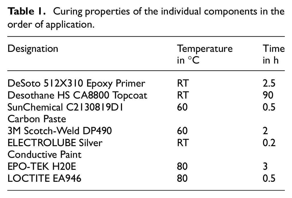
The prepared specimen is placed in an oven multiple times to complete the different preparation steps, as this ensures optimum properties of the individual components. In Table 1, the curing parameters of the individual components used in the preparation steps in the order of application are listed. Those components cured at room temperature are indicated with RT (22°C). The applied temperatures to complete the individual preparation steps are considered to cause no damages to the test specimen.

Table 1.

Curing properties of the individual components in the order of application.

Designation	Temperaturein °C	Timein h
DeSoto 512X310 Epoxy Primer	RT	2.5
Desothane HS CA8800 Topcoat	RT	90
SunChemical C2130819D1Carbon Paste	60	0.5
3M Scotch-Weld DP490	60	2
ELECTROLUBE SilverConductive Paint	RT	0.2
EPO-TEK H20E	80	3
LOCTITE EA946	80	0.5

Experimental procedure

The specimen prepared according to the preceding section is mounted on a test rig for mechanical loading. The test rig is placed in a laboratory environment where the ambient conditions are stable (typical moderate room temperature and humidity variations are present) to minimize their influence on the thin-film sensor. In Figure 2, the experimental setup, including the investigated CFRP plate with centrally placed circular hole and the used clamping fixture and hydraulic cylinder, the 3D-DIC system, and the EIT measurement system are illustrated. For the EIT reconstructions, an experimental framework, developed by the authors,³¹ is applied consisting of all components with which the EIT measurements and evaluations are performed. In this arrangement, the wiring of the elastoresistive thin-film sensor (frontside) is routed into a multiplexer, driven by an Arduino^® Mega 2560 (Arduino LLC, Boston, MA, US). This allows a defined current injection pattern in accordance with.³¹ As a current source, the Keithley^®6620 (Keithley Instruments, Cleveland, OH, US) is used. Measuring the resulting electrode voltages is performed with two HBM^® QuantumX MX840B (HBM, Darmstadt, Germany), which are operated simultaneously. In a computer, which is connected to the HBM QuantumX, the data acquisition and evaluation is carried out. These components are also depicted in Figure 2. The principle of the framework is described in a subsequent section, whereas a more detailed description is given in the studies by Wagner et al.^31,32 and Gschoßmann et al.³³

Figure 2.

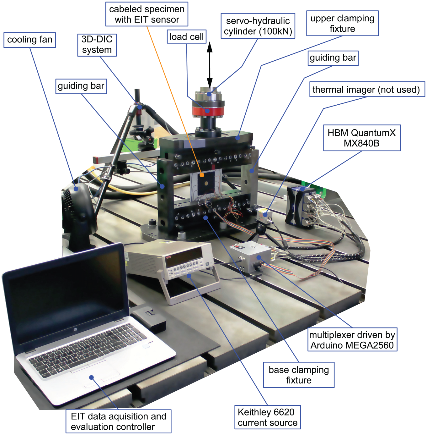
Experimental setup.

As illustrated in Figure 2, the plate is positioned in the center of the clamping fixture and held in place by tightening the clamping screws to avoid slipping out. The base part of the clamping fixture is attached to the test bed, and the upper part of the clamping fixture is attached to a load cell which is then loaded by a servo-hydraulic cylinder (Zwick Roell^® (Zwick Roell, Ulm, Germany); nominal force 100 kN). Lateral to the clamping fixture, guiding bars are provided on both ends to prevent the upper clamping fixture from rotating. The signals of the load cell are transmitted to a CUBUS controller (Zwick Roell) and used as control variable for the cylinder loading.

The plate is alternatingly subjected to a single quasi-static loading and a fatigue loading block of sinusoidal tension–tension loads. Within the repeated quasi-static loadings, the measurements for the damage evaluation from 3D-DIC and EIT are carried out. During the fatigue loading, no measurements are done; the cyclic loading is only used to induce realistic damage to the considered specimen and stress the sensor system. The repeated quasi-static loading is always the same for comparability of the measurements. The load levels of the fatigue loading blocks vary and are chosen to be comparable to previous results of the authors.³⁴ The associated strains are between 3000 and 12,000 μm/m and, thus, well represent a realistic operational loading of CFRP components, leading to realistic damage. In Figure 3, a schematic representation of a mechanical loading sequence i, composed of a single quasi-static loading and a cyclic loading, and a tabular list of the cyclic loading details are given.

Figure 3.

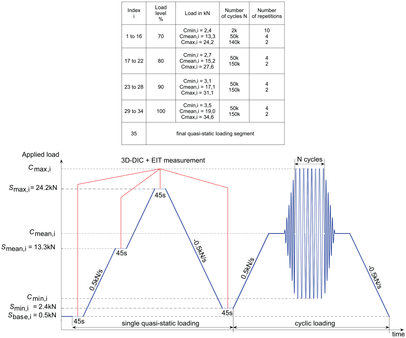
Tabular list of the loading details along with a schematic representation of a loading sequence i consisting of a single quasi-static loading for EIT and 3D-DIC damage evaluation and cyclic fatigue loading to provoke damage initiation and propagation.

For every quasi-static loading sequence, the load is raised to S_base,i = 0.5 kN where an EIT measurement is carried out and 3D-DIC images are taken. Here, the load remains constant for 45 s, providing adequate sampling time and allowing a data acquisition at constant loading conditions. To change the load to the other levels, it is changed with a rate of 0.5 kN/s. At (S_base,i, S_mean,i, S_max,i, S_min,i), the load remains constant for 45 s and EIT measurements and 3D-DIC images are taken to preserve comparability. Within the quasi-static loading, 3D-DIC images are taken at intervals of 500 ms each time when the load is held constant (see Figure 3). The two cameras of the 3D-DIC system (also indicated in Figure 2; provided by Correlated Solutions) are focused on the speckled area of the specimen with circular hole (backside).

After the quasi-static loading, the cyclic loading starts. Cyclic loading is implemented with a frequency of 4 Hz and a stress ratio of $R = 0.1$ . To introduce and end the cyclic loading between C_max,i and C_min,i with less intensity, five Fade-In cycles and five Fade-Out cycles at the beginning and at the end of the cyclic loadings are added. After completing the defined number of cycles (N_i), the load is reduced to S_base,i+1 and the next quasi-static and cyclic loading (i + 1) is performed. The loading sequences are carried out until the specified number of repetitions is completed. After every 500k fatigue load cycles, the cyclic loading is raised by 10%. Following 2000k cycles, a final quasi-static loading is done (i = 35), with which damage at the test end is evaluated.

Damage evaluation by DIC (3D-DIC)

The speckled area on the backside of the specimen with centrally placed circular hole is utilized to evaluate occurring damage due to the cyclic loading. These evaluations are used to validate the EIT reconstructions. 3D-DIC evaluation is performed by comparing images that are taken with two cameras simultaneously. Both cameras are arranged at different angles to the specimen surface to allow a 3D correlation. Comparisons of images or regions within the images (evaluated area) at different load states or cycles allow one to calculate changes with respect to the reference images. This calculation (named correlation) is carried out on subsets, which are groups of several pixels (pixel is the smallest addressable element of a rasterized images). The individual subsets are tracked by the gray value of the pixels that are within the subsets. The use of two 5 Mpx industrial cameras (grayscale cameras) means that each image consists of 2592 × 1920 pixels (px). The selection of a subset of 29 px consequently divides the individual images in 29 × 29 px areas (=subsets) for which the correlations are performed. Usually, a step size of 1/4 of the subset size is specified. Thus, the step size defines the smallest level of discretization for which the correlations are determined (e.g., displacements and strains). During the evaluations, the spatial one-standard deviation confidence in the correlation (correlation confidence) is also computed, which can be utilized to determine the quality of the match of the individual subsets.^35,36 To the extent that the subsets (gray values) are changed (e.g., noise, changes in lighting, and spatial changes to the speckled area or displacements of the specimen), the correlation confidence is reduced.^37,38 Other changes, like, for example, cracks, also cause a reduction in the correlation confidence. Thus, this quantity is frequently considered as an indicator for damage.^34,39,40

To evaluate potential damage, the spatial surface strains are evaluated from the acquired images taken at the quasi-static loading. In this process images of the base load, S_base,i are correlated with that of the peak load S_max,i. An evaluation of the individual single quasi-static loadings reveals any changes inside the spatial strain field and might be an indicator for cyclically induced damage. The first image at the corresponding base load S_base,i is taken as reference image. In Figure 4, the evaluated area, the selected subset size, and the associated settings are shown.

Figure 4.

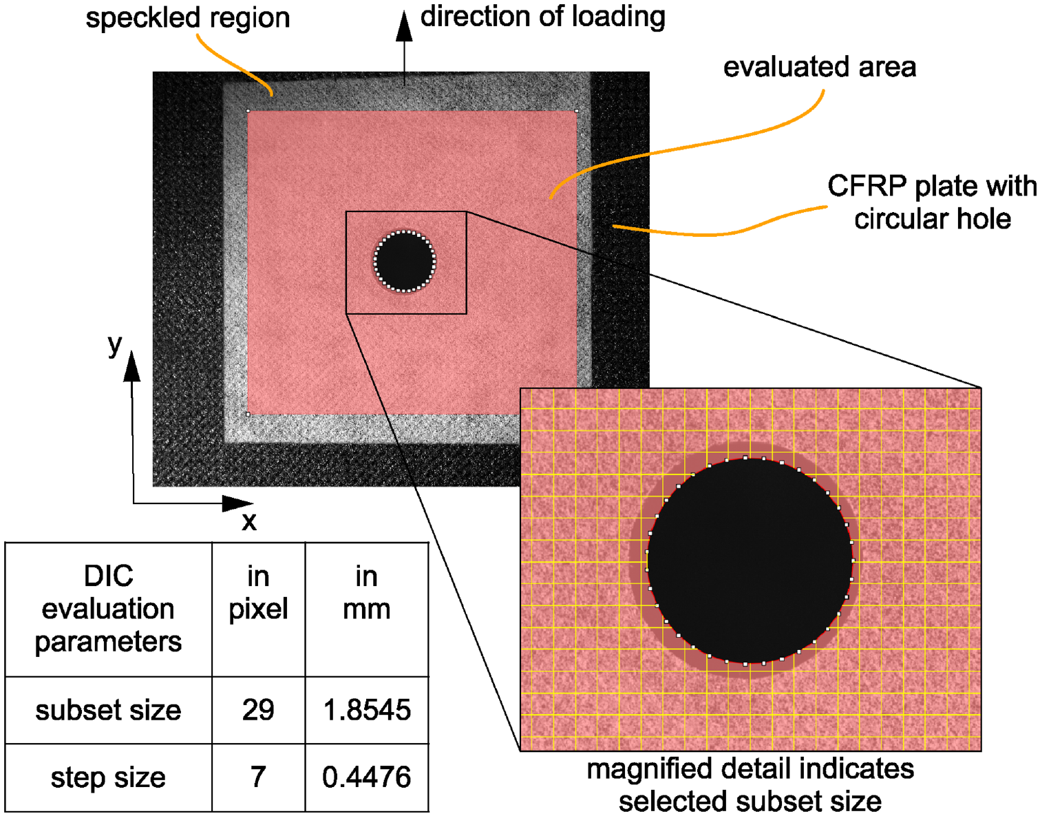
Positioned evaluated area, magnified detail to visualize the subset size and associated settings.

Additional 3D-DIC evaluations are carried out in which the correlation confidence is utilized as an indicator for damage, as this allows an approximation of the area of damage. In this case, it is necessary to be aware that the correlation confidence is load dependent. Thus, to avoid the effect of loading on the correlation coefficient, evaluations of 3D-DIC images taken at the same load level (S_max,i) are conducted. As a reference image, the first image (i = 1) at peak load S_max,i is taken, and subsequently, all images at different cycles are correlated with this. For the reference image, the same evaluated area and associated setting as for the strain evaluation (see Figure 4) are used. The continuous acquisition of images (45 s) at each quasi-static loading allows an averaging to reduce noise. Due to the evaluations of 3D-DIC images taken at the same load level (S_max,i), changes to the correlation confidence are attributed to damage, since it is assumed that any other influences on the correlation confidence are negligible with the selected evaluation. For every image, a dataset containing the correlation coefficient values and a cycle number is exported. Entries of the correlation coefficient that exceed a predefined threshold value are summed up and multiplied by the step size (using the metric unit, as given in Figure 4) to obtain an area. This procedure is used to determine the shape and size of the damage for each evaluation. By assigning the number of cycles, a damage progression can be depicted. This method was already demonstrated in the studies by Heinzlmeier et al.^34,41

Damage evaluation by EIT

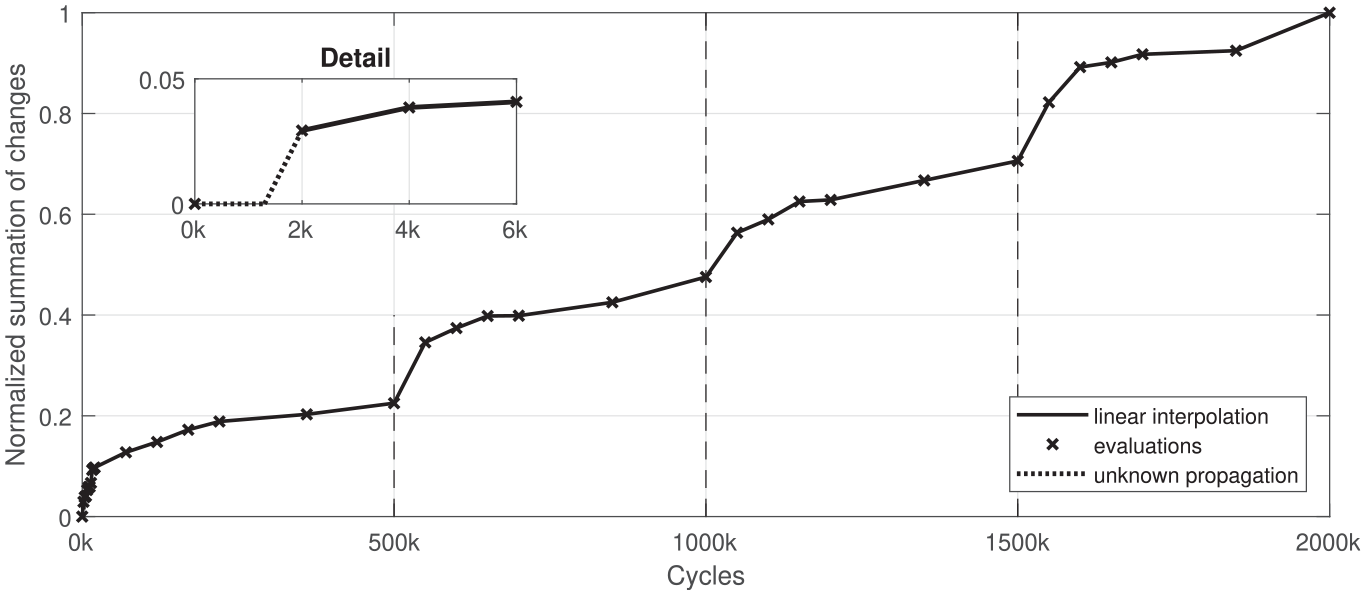
Contrary to the 3D-DIC damage evaluations, where an evaluation is performed on the entire evaluation area, the EIT reconstructions are performed only from data collected at the boundaries (measurements at electrodes). As a result, the EIT can only provide an estimation of the spatial conductivity changes. Therefore, the elastoresistive thin-film sensor is used to carry out differential EIT reconstructions of the spatial conductivity changes. In this way, systematic voltage measurements on the placed electrodes are performed throughout the experiment and give the boundary potential to solve the inverse solution. The EIT evaluation framework for measurement data collection, preprocessing, and conductivity reconstruction was developed in a previous work.³¹ In this process, the Gauss–Newton one-step algorithm is utilized to solve the differential inverse EIT reconstruction using a maximum a posteriori regularization approach.^42–44 In Equation (1), the resulting linearized inverse EIT approach is given.

Δ \hat{σ} = {(H WH + λ^{2} Q)}^{- 1} (H W) Δ v

(1)

This approach involves the Noser prior for regularization. The estimated change of the spatial conductivity $Δ \hat{σ}$ is obtained via the change of voltage potentials at the boundaries $Δ v$ (electrodes). Additional variables in Equation (1) are the sensitivity matrix $H$ , the weight matrix $W$ , the regularization matrix $Q$ , and the hyperparameter $λ$ , which help to solve the differential inverse linearized problem. The choice of the hyperparameter is a key element for the EIT reconstruction. Selection of the hyperparameter was based on the same method as that presented in Wagner et al.³² The hyperparameter is deliberately kept constant for all reconstructions in order to obtain a simple (linearized differential EIT reconstructions) and robust (consistent parameters) EIT solving framework. For the investigation performed within this article, the hyperparameter is defined as λ = 1.8307 × 10⁶. A detailed description of the underlying experimental framework and evaluation process can be found in the study by Wagner et al.³¹

However, the EIT-based damage reconstruction of realistic operational fatigue loading faces challenges due to the thin-film sensor material’s “Set-In” effect and other sensor-related environmental influences (e.g., temperature or moisture). To overcome this issue, two evaluation approaches are investigated to demonstrate the EIT method for SHM application under fatigue and operational loading, respectively.

Fatigue damage evaluation using mean value adjustment. In line with the 3D-DIC evaluation of damage, the EIT measurements at the same load level but at different numbers of cycles are taken for the systematic differential EIT reconstructions. As reference, the EIT measurements of the first quasi-static loading are taken (e.g., the measurements at S_base,1, S_mean,1, S_max,1). Due to the fact that each differential EIT reconstruction refers to the first measurement, the cycle and strain dependent initial conductivity change of the sensor material affects the damage evaluation and needs to be considered. The associated effect is better known as the “Set-In” effect³⁰ and strongly influences the reconstruction results. However, assuming the “Set-In” effect to be homogeneous over the sensor area, and furthermore, assuming the influence of the damage on the mean conductivity to be small and not affecting the elastoresistivity, allows one to compensate its influence by $Δ {\hat{σ}}_{comp, i} = Δ {\hat{σ}}_{i} - (mean ({\hat{σ}}_{i}) - mean ({\hat{σ}}_{1}))$ .

Thereby, the “Set-In” compensated conductivity change of the sensor $Δ {\hat{σ}}_{comp, i}$ is obtained by subtracting the difference of the ith mean conductivity of the sensor $mean ({\hat{σ}}_{i})$ and the initial mean conductivity of the sensor $mean ({\hat{σ}}_{1})$ from the ith conductivity change of the sensor $Δ {\hat{σ}}_{i}$ .

The mean conductivity of the sensor is determined using the Montgomery method.⁴⁵ Thereby, the absolute conductivity is determined on the basis of the same measurement data used for the differential EIT reconstructions.³¹ The deviation from the originally published Montgomery method is considered acceptable because the sensor shape remains consistent over the experimental investigation.

This mean value adjustment could also compensate for other environmental influences on the sensor’s conductivity, like, for example, temperature and humidity, as long as the sensor area is homogeneously affected, and the elastoresistivity remains unaffected. Resulting spatial conductivity changes can be related to potential damage. Identification of this spatial conductivity change is performed with a conductivity change threshold.

Fatigue damage evaluation using continuous reference measurement adjustment. Alternative of using a single reference EIT measurement, several EIT measurements as references can be used in order to evaluate potential damage. In this way, the “Set-In” effect and also potential other environmental influences on the sensors conductivity can be compensated. Compared to the mean value adaption method, the adaption of the reference measurement can also compensate inhomogeneous conductivity changes. However, also this method requires the assumption of an unaffected elastoresistivity. To investigate this proposed approach, EIT measurements at base load S_base,i are related to measurements at subsequent peak load S_max,i, and EIT measurements at base load S_base,i are related to measurements at subsequent mean load S_mean,i. As the reconstructions are based on measurements at different load levels, the spatial conductivity changes are a combination of mechanical loading and potential damage. For damage evaluation, solely the negative component of the spatial conductivity changes is utilized, as it is assumed that only a reduction in conductivity changes reflect potential damage.

Results

This section presents the results of the validating 3D-DIC-based shape and size evaluation and the EIT-based evaluation of the initiating and propagating damage.

As part of the experimental investigation of the plate with a circular hole, validating 3D-DIC evaluations are performed on the backside and EIT reconstructions on the frontside. Since no fracture of the specimen or measurement error due to a chipped electrode has been encountered, damage evaluation could be carried out throughout the entire test duration. In addition, the electrical contacts did not show any visible deterioration after the test.

During the test, free-edge delaminations were visually observed at the two highly stressed hole sides. First observation of the delaminations was approximately after 1500 cycles at the left side of the highly stressed hole. Shortly afterward, after 2000 cycles, delaminations were also observed at the opposite side of the hole. Both delamination sites could be visually observed to continuously grow in size and number of delaminated plies. These results perfectly correlate with the findings presented for the same plate and loading in a previous work.^34,41 Furthermore, a post-test analysis of the specimen’s speckled surface around the hole using an optical microscope also revealed surface cracks. These cracks are aligned with the fiber bundles and most probably intralaminar matrix cracks that evolved from the propagating delaminations. However, a more detailed investigation of the damage behavior is not part of the present study.

3D-DIC damage evaluation results

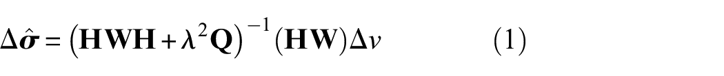
Evaluated changes inside the spatial surface strain field are considered as indicator for cyclically induced damage.Performed evaluations (S_base,i to S_max,i) yield to strain fields like those exemplarily illustrated in Figure 5. Thereby, the spatial distribution of the major principal strain $ε_{1}$ is plotted for chosen cycles. The selected color bar remains unchanged to highlight the strain field alteration in the vicinity of the circular hole.

Figure 5.

3D-DIC evaluated major principal strain $ε$ 1 at different cycles (evaluated from S_base,i to S_max,i).

As cyclic fatigue loading continues, the 3D-DIC-evaluated strain field also changes, although the considered static load level does not. In particular, the areas with high strains become larger in those regions that are exposed to the stress concentrations at the hole. This can be interpreted as an indicator of existing damage, which becomes apparent by selecting the upper scale level at 10,000 μm/m (maximum strain allowable for used plies), and observing how the red area (all strain values above 10,000 μm/m) evolves over the increasing number of cycles. However, the used threshold is very high, and thus, according to the strength properties of the laminate, material degradation must be present in the plies at these regions. This is also supported by the surface cracks found in the post-test analysis, as these were only found in the regions strained above 10,000 μm/m at the test end. Thus, the increase of the highly strained area represents the propagating damage, although it may not reflect its true size and shape.

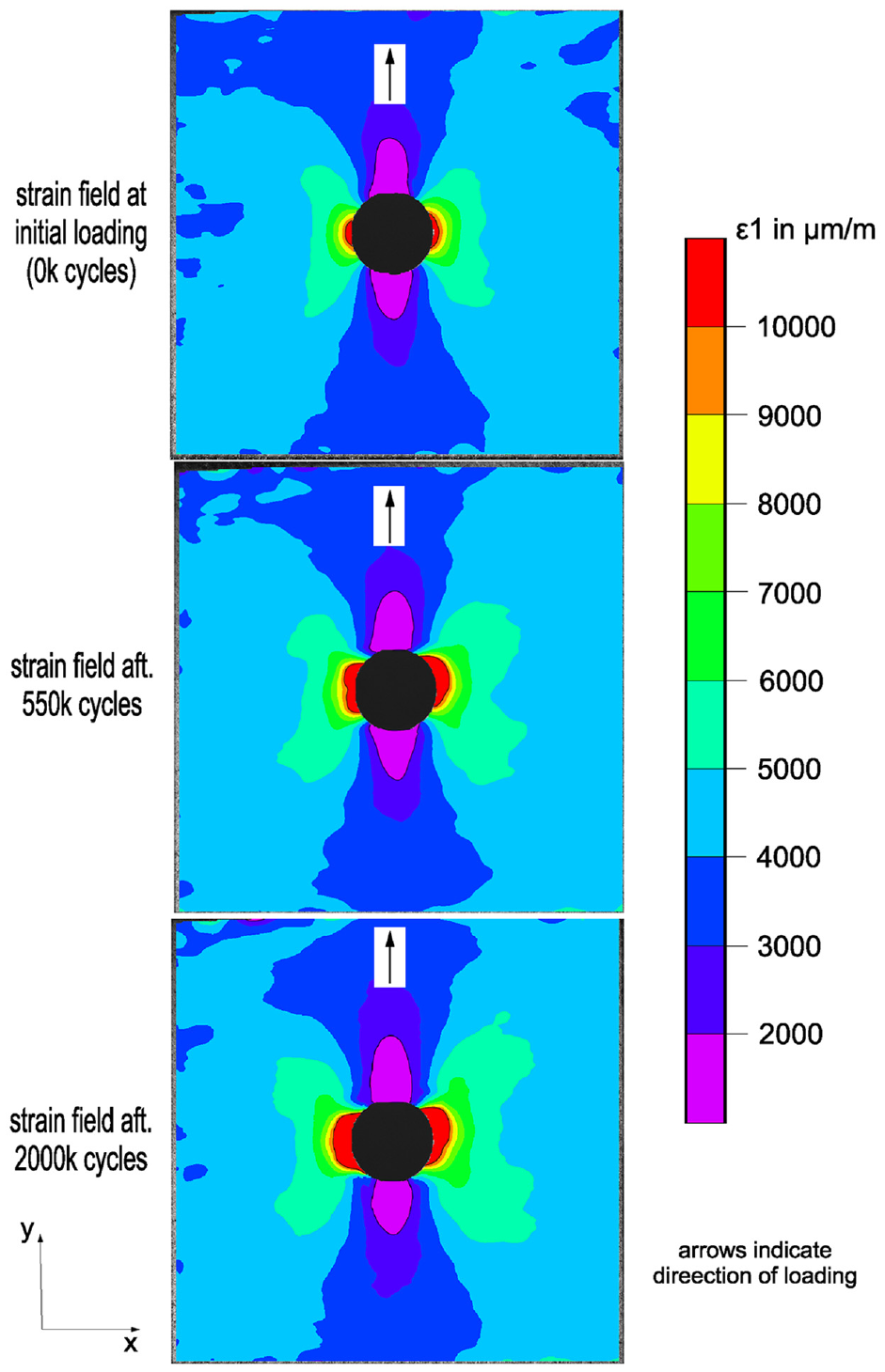
In order to demonstrate changes in the spatial surface strain field throughout the entire test, a summation of all spatial strains at which the upper scale level (10,000 μm/m) is exceeded and a multiplication with the step size (metric unit) is performed. The resulting damage-affected changes in the spatial surface strains are normalized with respect to the last evaluation and are shown in Figure 6.

Figure 6.

Normalized changes in the spatial surface strains (major principal strain $ε_{1}$ ) versus the test length for S_base,i to S_max,i from 3D-DIC evaluations.

From Figure 6, it is obvious that the damage already initiates before 2k cycles. This is supported by the fact that the predefined threshold value is exceeded at 2k cycles, which means that damage has occurred. Since only an evaluation at 2k cycles is performed, a more accurate evaluation of damage initiation and early damage propagation (within the first 2k cycles) is not possible. In Figure 6, this unknown propagation is represented by a dotted line, which, however, only serves as a qualitative indication. Thereafter, the damage-affected changes in the spatial surface strains become larger, as the number of cycles increases. This increase continues continuously throughout the fatigue loading. Within the different fatigue load levels, a systematic behavior is observed, with an initially more pronounced increase followed by a decelerating behavior as cyclic loading continues. Irrespective of the fact that this evaluation does not provide an actual damage size, it can be considered to qualitatively represent the changes, and thus the damage, resulting from fatigue loading.

A good and readily demonstrated approximation of the size and shape of the damage is provided by the spatial correlation confidence.³⁴ Comparing measurements acquired during the experimental investigation under the same load, but after an increasing numbers of fatigue cycles, provides information on damage initiation and damage propagation. All images obtained at peak load S_max,i are evaluated independently with respect to S_max,1. In Figure 7, exemplarily 3D-DIC evaluation results after different numbers of cycles are depicted. The color shading represents the evaluation’s spatial correlation confidence and is fixed. As threshold level for damage, a correlation coefficient of 0.01 is selected, as this value was validated on identical specimens subjected to identical loads in a previous work.^34,41

Figure 7.

3D-DIC evaluation results for S_max,i with respect to S_max,1. The defined correlation confidence threshold reveals the damage shape and size (red region).

The 3D-DIC evaluations depicted in Figure 7 indicate that damage initiation already occurs before 2k cycles and that damage propagation takes place throughout the length of the experiment. Observing the vicinity of the hole reveals that the threshold surpassing area (red region) becomes larger. The red regions away from the hole do not correspond to any damage, but are attributable to a local overexposure, and thus do not change throughout the experiment.

Summing up all portions where the defined threshold value (0.01) is exceeded, multiplication with the step size (metric unit) yields to the area of damage for discrete cycles. The obtained path of damage progression based on the area of damage is normalized with respect to the maximal area of damage (37.89 mm², evaluated by the same method) that is found and is presented in Figure 8.

Figure 8.

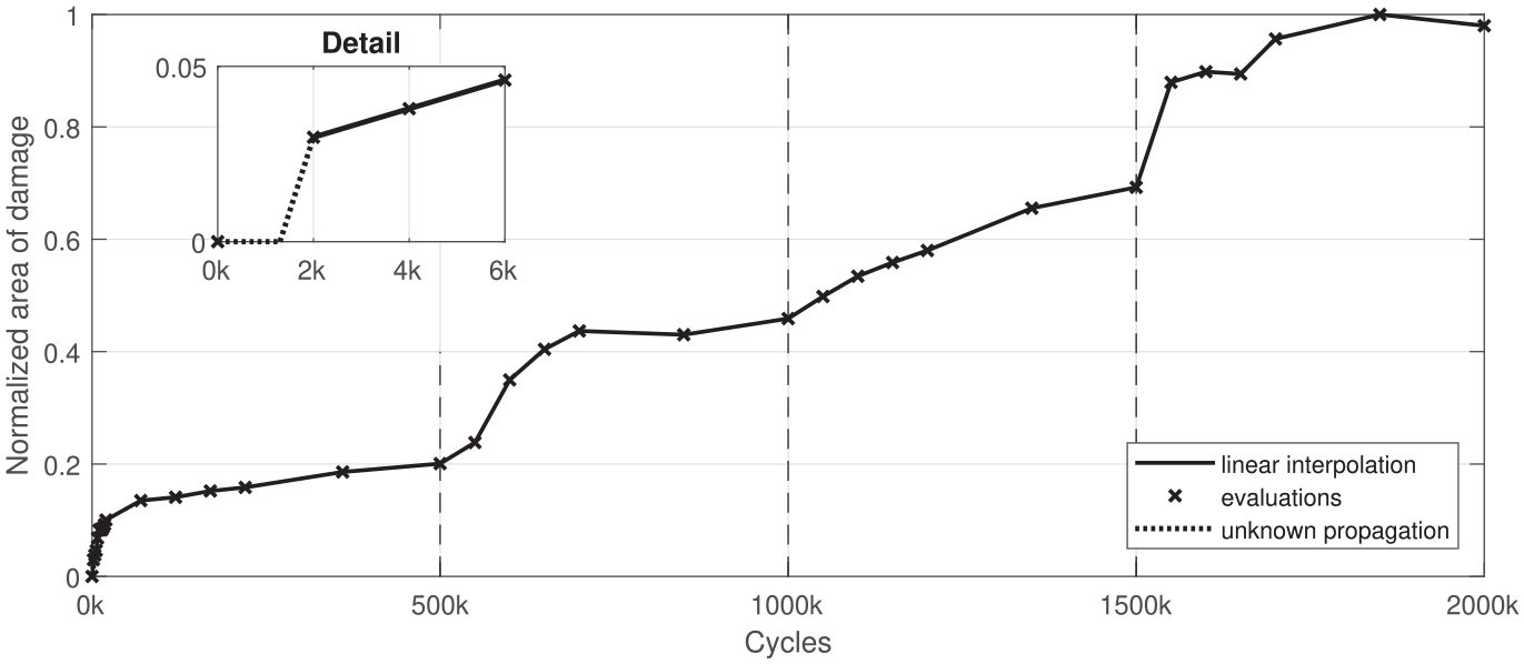
Normalized 3D-DIC evaluated damage size for quasi-static load level S_max,1 with respect to S_max,1 over the number of cycles.

Within the first 2k cycles (see detail in Figure 8), damage initiation is observed, as at this cycle count, an initial increase in the area of damage is present. However, the exact cycle number of damage initiation cannot be identified. Again, the unclear cycle number of damage initiation and unclear propagation (up to 2k cycles) is indicated as dotted line. Thereafter, damage propagation takes place and continues over 500k cycles. At 500k cycles, the identified damage size is in agreement with the findings of a previous work.³⁴ Afterward, the load dependence of the correlation confidence is present, since the static load S_max,i and the cyclic load C_max,i are not identical (load increase by 10% after every 500k cycles), and thus, the identified damage no longer corresponds to the actual damage. This means that the damage caused by C_max,i is slightly larger than that evaluated at S_max,i. Nevertheless, a qualitative evaluation of the damage growth is possible based upon the correlation confidence.

EIT-based fatigue damage evaluation results

Within this section, the results of the two approaches are presented, with which sensor conductivity changes due to fatigue loading and other potential environmental influences can be compensated.

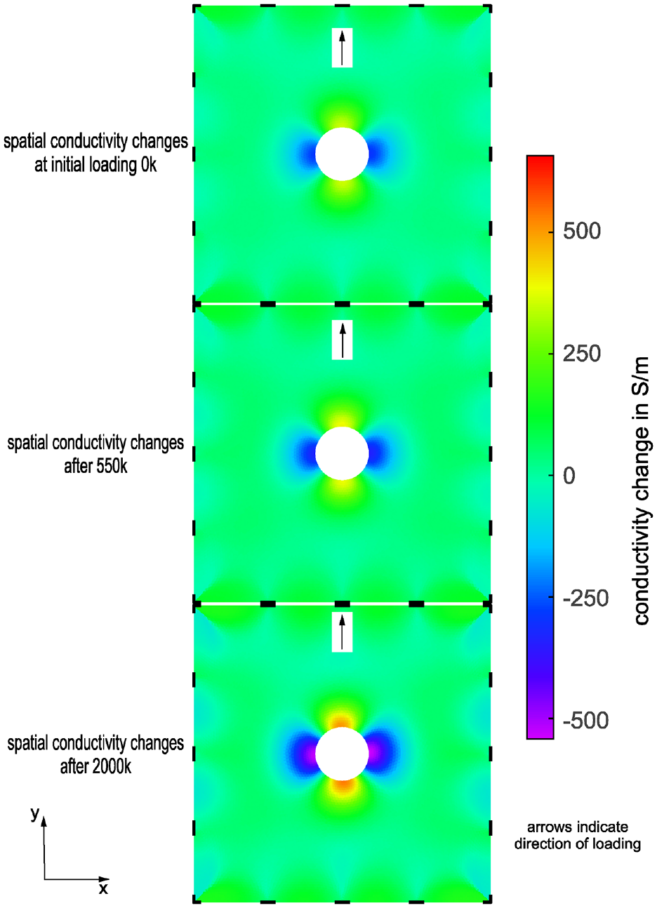
Damage reconstruction using mean value adjustment. All EIT measurements carried out at the quasi-static loadings (mean load S_mean,i and at peak load S_max,i) are evaluated individually with respect to the measurements at the initial static loading (S_mean,1, S_max,1). For the given laboratory setup with constant temperature and humidity, these differential EIT reconstructions provide the sole electrical conductivity change of the elastoresistive thin-film sensor. The resulting conductivity changes of the sensor are accounted by two phenomena, whereby the initially dominant “Set-In” effect is compensated at this proposed approach. Remaining portions of the negative component of the spatial conductivity changes are attributable to potential damage. In Figure 9 exemplarily, the EIT reconstructions of the “Set-In” compensated spatial conductivity changes for selected cycles (index i allows a cycle assignment) at peak load S_max,i are depicted. The used scaling remained unchanged to visualize spatial conductivity changes that are attributable to potential damage.

Figure 9.

Spatial conductivity changes at peak load S_max,i for selected cycles.

In the evaluations of these EIT reconstructions, partial increases in conductivity (attributable to compressive strains) and local decreases in conductivity (due to tensile strain and potential damage) are present. Besides these observations, a conductivity decrease at the sensor electrodes can be observed. However, this is due to the numerically linearized EIT reconstruction algorithm and measurement noise and, therefore, can be neglected. Nevertheless, Figure 9 reveals clear changes in the spatial conductivity throughout cyclic fatigue loading.

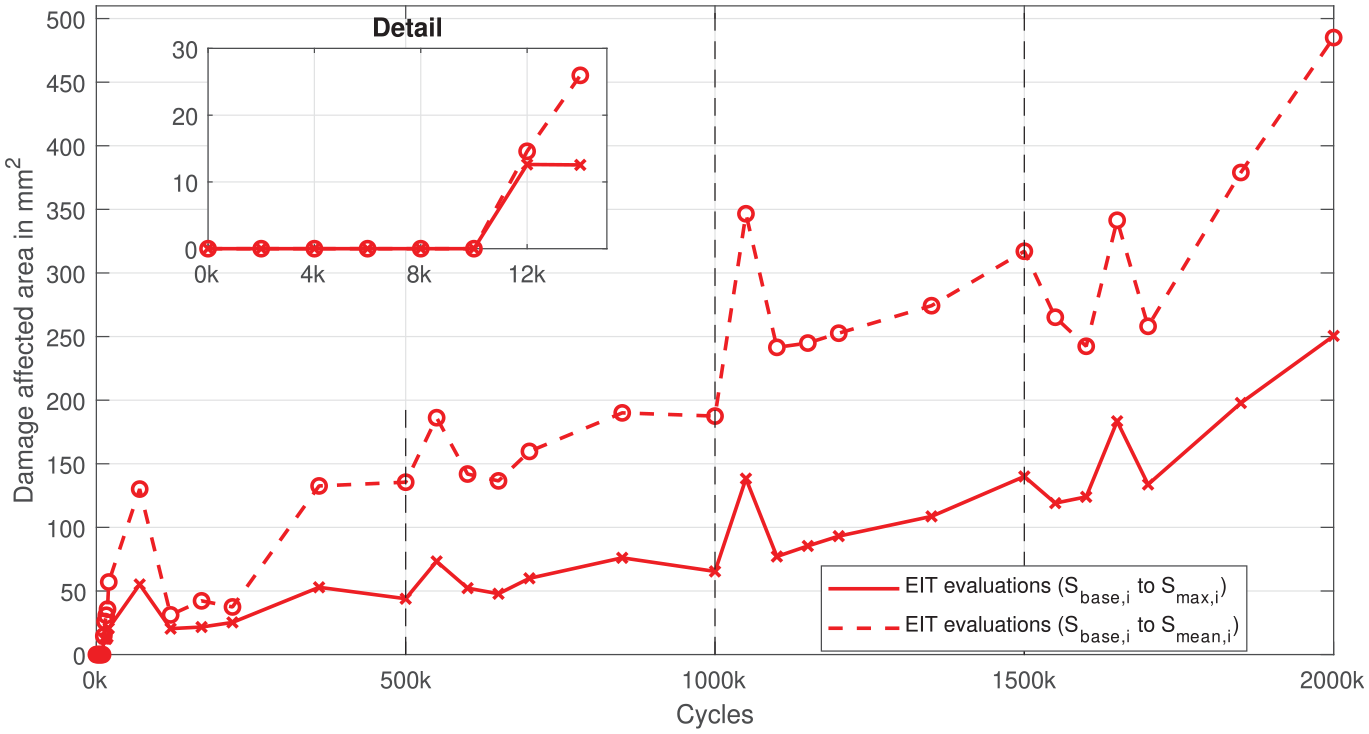
Based on an initial EIT reconstruction of the unloaded thin-film sensor (before the first quasi-static loading), the conductivity change threshold to identify potential damage is ascertained by −53 S/m. The conductivity change threshold is chosen to represent 10% of the initial conductivity of the unloaded sensor. A summation of all spatial conductivity changes below this threshold provides information on the damage propagation over the number of cycles. In Figure 10, the summarized threshold exceeding spatial conductivity changes is plotted over the number of cycles.

Figure 10.

Area of conductivity changes below threshold value over the number of cycles for S_mean,1 to S_mean,i and S_max,1 to S_max,i.

Due to the mean value adaption of the EIT reconstructions, the “Set-In” effect is compensated. Potential further environmental influences (e.g., temperature and moisture) stay constant at the institute’s test rig and, thus, can be excluded. Consequently, as the EIT measurements are taken at the same load levels, resulting decrease within the spatial conductivity is predominantly the result of an increasing damage. Both the spatial conductivity changes at mean load S_mean,i and peak load S_max,i show that as the test duration advances, the spatial conductivity decreases. Spatial conductivity changes evaluated at mean load S_mean,i follow an identical trend to that at peak load S_max,i, also indicating an increasing damage. From both paths, a first drop of the conductivity is observed after 10k to 12k cycles. The spatial conductivity changes rapidly but slows down with an increasing number of cycles at the first cyclic load level. The same behavior can also be observed for every load increase (by 10% every 500k cycles), where the spatial conductivity change is more pronounced, before it slows down again. Conversely, when the load is adjusted to 100% (at 1500k cycles), there is no pronounced spatial conductivity change. Due to the definition of the conductivity change threshold (10% of the initial conductivity of the unloaded sensor), only spatial conductivity changes that cause a more significant drop are accounted, so that no spatial conductivity changes are determined up to 12k cycles (see detail in Figure 10). Consequently, the detection of damage initiation by the proposed EIT-based method is less sensitive than the 3D-DIC system. Additionally, the absence of the measurement at 0k cycles is apparent, which is attributable to the differential EIT reconstruction.

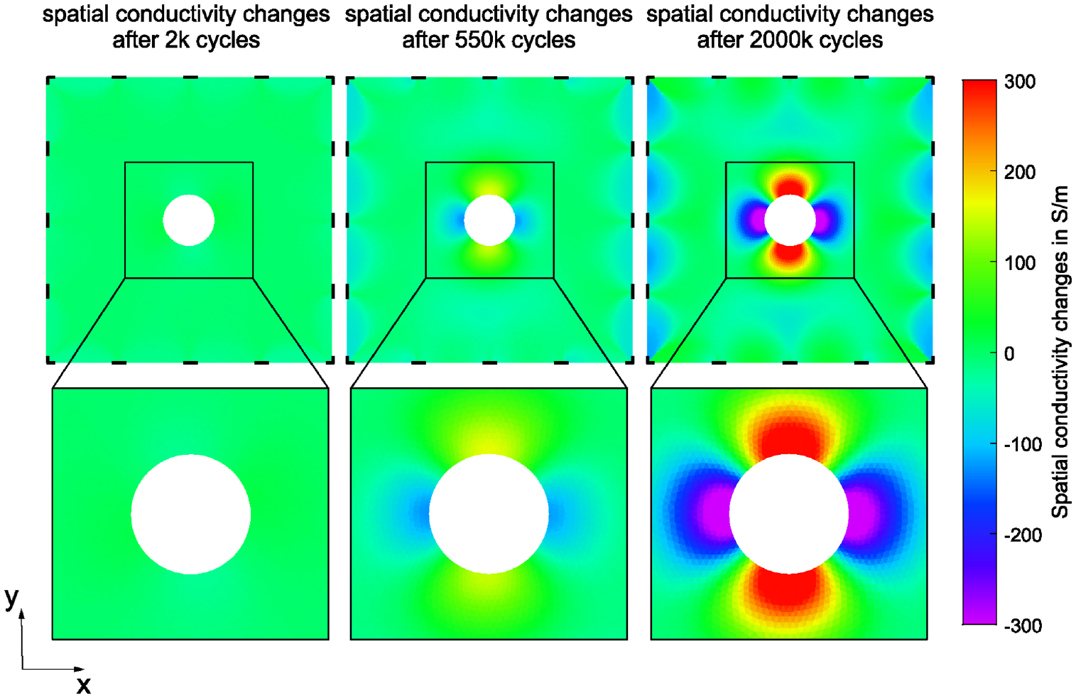
Damage reconstruction using continuous reference measurement adjustment. The damage evaluation by continuously updated EIT reference measurements also allows the compensation of the “Set-In” effect and other possible environmental influences on the sensor material conductivity. As stated earlier, the resulting spatial conductivity change reconstructions reflect a combination of potential damage and strain due to the mechanical loading, as measurements at S_base,i are used as reference and the immediately following measurements at S_max,i or S_mean,i are used to calculate the differential potential at the boundaries. In Figure 11, the EIT reconstructions of the spatial conductivity changes after different numbers of cycles are exemplarily depicted for three isolated cases, where S_base,i to S_max,i are evaluated.

Figure 11.

EIT reconstructions of the spatial conductivity changes at different cycles (evaluated from S_base,i to S_max,i).

In the areas of higher stresses, where also the delaminations and surface cracks were observed (at the hole, perpendicular to the loading direction), the EIT reconstructions reveal a decrease in spatial conductivity. In the initial evaluation before fatigue loading, this decrease in spatial conductivity can be assigned to the pure mechanical strain due to the loading; however, it becomes more pronounced with increasing number of cycles, which can only be explained by formation and growth of damage. In contrast, the spatial conductivity increases in the areas exposed to compressive stresses (at the hole, in loading direction; see Figure 5). This local increase in spatial conductivity is accounted to the compressive strains and mainly to artifacts during the reconstructions. Similarly, boundary effects at the electrodes are present, but they are not considered.

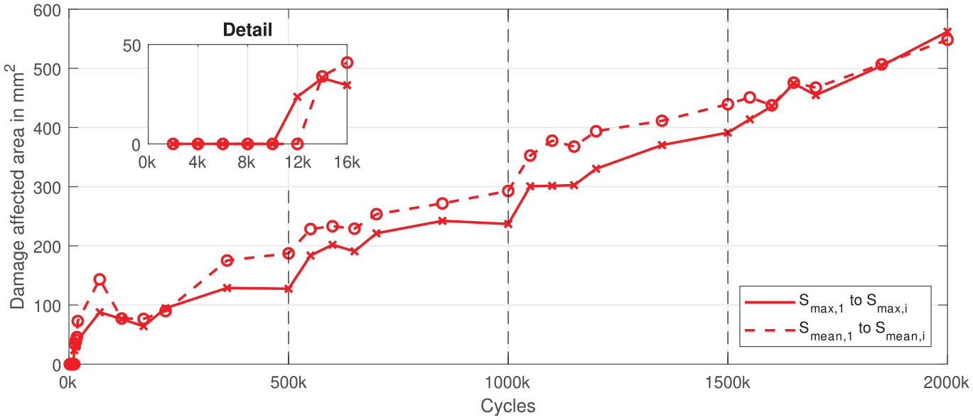
In order to indicate the alterations in spatial conductivity changes over the cyclic fatigue loading, threshold values are specified that allow a summation of the damage-affected sensor area for the individual reconstructions. The threshold values are defined as the minimum of the negative component of the spatial conductivity change at the first EIT reconstructions. Accordingly, the threshold value to describe spatial conductivity changes from S_base,i to S_max,i is $- 341.80 S / m$ , and for S_base,i to S_max,i, it is −153.82S/m. In Figure 12, the assumed damage-affected area (sum of all elements that exceed the defined threshold) is plotted over the number of applied fatigue cycles for both evaluations.

Figure 12.

Damage-affected area over the number of cycles for S_base,i to S_max,i and S_base,i to S_mean,i EIT reconstructions.

Here, consistent with Figure 11, where selected reconstructions are given, the negative component of the spatial conductivity changes is found to grow throughout the cyclic fatigue loading. This corresponds to an increase in the damage-affected area as indicated in Figure 12. This outcome is obtained from both evaluations that have been carried out. The results derived from the evaluations at S_base,i to S_mean,i provide a more pronounced increase than that at S_base,i to S_max,i. Each time the cyclic load is increased, significant changes in the development of the EIT-evaluated damage-affected area take place. After these temporary more pronounced changes, the EIT-evaluated damage-affected area subsides thereafter, but indicates a continuous increase. As a consequence of the thresholds being defined, no alteration in the EIT-evaluated damage-affected area is found in the first 10k cycles (see detail in Figure 12); thus, the potential damage initiation was detected later that observed by the 3D-DIC system.

Discussion

The damage induced by the cyclic fatigue loading is evaluated by measurements taken in the quasi-static loadings. As evaluations of the spatial surface strain field by 3D-DIC reveal, degradation in the vicinity of the hole occurs, providing an indication of existing damage. While Figure 5 shows this degradation for isolated cases, visualization of the degradation throughout the entire cyclic fatigue loading is achieved with a threshold value (see Figure 6). To identify the shape and size of the underlying damage with 3D-DIC, the correlation coefficient is used. The resulting path (determined with a threshold value), given in Figure 8, serves as a qualitative comparative quantity for the EIT evaluations.

This path, obtained by the 3D-DIC correlation coefficient, reveals damage initiation at the edge of the circular hole within the first 2k cycles (see detail in Figure 8). This observation is in agreement with previous findings of the authors³⁴ where detailed focus was placed on damage initiation and propagation of similar specimens subjected to a single cyclic loading amplitude. The adopted threshold value also shows a comparative damage size at 500k cycles. Thereafter, the load dependency of the correlation confidence is present. Meaning that the arising delaminations and micro-cracks induced by higher cyclic loadings are not fully opened within the quasi-static loading, where the evaluation takes place This is owed to the fact that the quasi-static loading (70%) is below the cyclic loading (80%, 90%, 100%). Thus, implying that the actual size of the damage is larger than that obtained from 3D-DIC evaluation, as for all cyclic loadings the 3D-DIC evaluations at quasi-static loading (70%) are considered, although higher cyclical loads were applied (80%, 90%, 100%). Nevertheless, the tendency of damage progression is still present throughout the cyclic fatigue loading.

Before the results of the 3D-DIC evaluations and the EIT reconstructions are compared, the results of the EIT reconstructions are verified to ensure that they are not due to degradation of the sensor itself. Therefore, the baseline measurements S_base,i are examined individually to obtain the mean spatial conductivity of the sensor using the Montgomery method. In Figure 13, the mean spatial conductivity of the sensor is plotted over the number of cycles.

Figure 13.

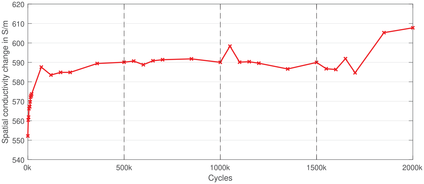
Mean spatial conductivity of the thin-film sensor (evaluated with the Montgomery method) for S_base,i evaluations, indicating the “Set-In” effect at the beginning and a stable sensor conductivity up to 1750k cycles.

At the initial 70k cycles, the “Set-In” effect is evident. Owing to this strong initial conductivity change, there is also no precise identification of the damage initiation, since it occurs within the first 2k cycles as indicated by the 3D-DIC evaluation. Likely the small extent of the damage at initiation may also influence the detectability, meaning that an evaluation by means of EIT may be possible only for damage above a certain size. After the “Set-In” effect, it appears that the conductivity of the sensor remains relatively stable and allows the evaluation of damage progression. Additionally, this indicates the suitability of the used thin-film sensor material for this application and that the obtained results are primarily attributable to spatial conductivity changes, caused by, for example, potential damage. After 1750k cycles, the spatial conductivity of the sensor starts to increase, indicating a possible degradation of the sensor. However, further investigations are required to obtain more detailed information about the service life of the used sensor.

The results of the first proposed approach given in Figures 9 and 10 are obtained by referring EIT measurements taken at the same load level but at different cycles to an initial measurement (i = 1). Here, the compensation of the strong initial conductivity change (e.g., “Set-In” effect) is conducted. In contrast, environmental influences (e.g., humidity and temperature) that may occur are not accounted within this approach.

Using the area of spatial conductivity changes from Figure 10 and scaling them to reflect the normalized damage size from the 3D-DIC evaluation at 1500k cycles allow a common representation. In Figure 14, the EIT reconstructions (also presented in Figure 10) and the 3D-DIC evaluation (also presented in Figure 8) are given to validate the outcome of the EIT reconstructions. Here, the EIT-based damage evaluation results using mean value adjustment as described are used.

Figure 14.

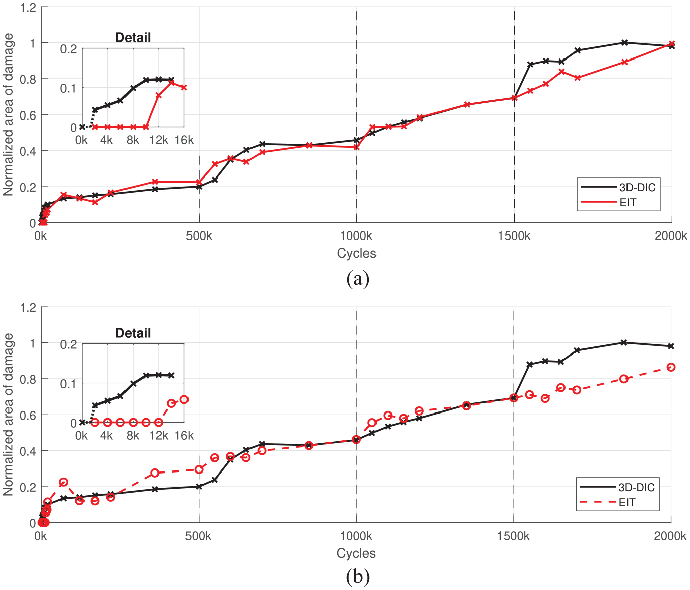
3D-DIC-based validation of EIT-based damage evaluation results using mean value adjustment for (a) S_max,1 to S_max,i and (b) S_mean,1 to S_mean,i.

This common representation reveals that the spatial conductivity changes correlate very well with the 3D-DIC outcomes. Comparing the 3D-DIC results with those of the EIT reconstructions at peak load S_max,i yields a significantly stronger agreement than with those at mean load S_mean,i. Up to 1500k cycles, both EIT reconstructions show satisfactory agreement; beyond this cycle number, the differences between 3D-DIC and EIT become larger. This may indicate a deterioration of the thin-film sensor, which is also supported by the mean spatial conductivity change given in Figure 13. This also explains the scaling of the EIT reconstructions at 1500k cycles. Nevertheless, both comparisons emphasize that EIT reconstructions can also be used to evaluate the damage progression, to the extent that the initial strong conductivity change is taken into account, as shown in the first proposed approach.

The second approach is based on a continuous adjustment of the reference measurement. In this process, the baseline measurement S_base,i is updated, and subsequent measurements at peak load S_max,i and mean load S_mean,i are referred to this. As the respective measurements are carried out under the same conditions and with the same number of cycles (indices i), environmental influences and the “Set-In” effect can be excluded. Thereby, evaluated spatial conductivity changes are the result of a superposition of mechanical loading and potential damage. Results presented in Figure 12 reveal an increase of the damage-affected area over the number of fatigue cycles. Using these results and scaling them in accordance with the normalized 3D-DIC results from Figure 8 provide a combined representation, as given in Figure 15. Again, the 3D-DIC result at 1500k cycles is used for scaling the EIT results. In Figure 15(a), the 3D-DIC evaluations are plotted besides the EIT reconstructions of the S_base,i to S_max,i evaluations. In Figure 15(b), the 3D-DIC evaluations are plotted besides the EIT reconstructions of the S_base,i to S_mean,i evaluations.

Figure 15.

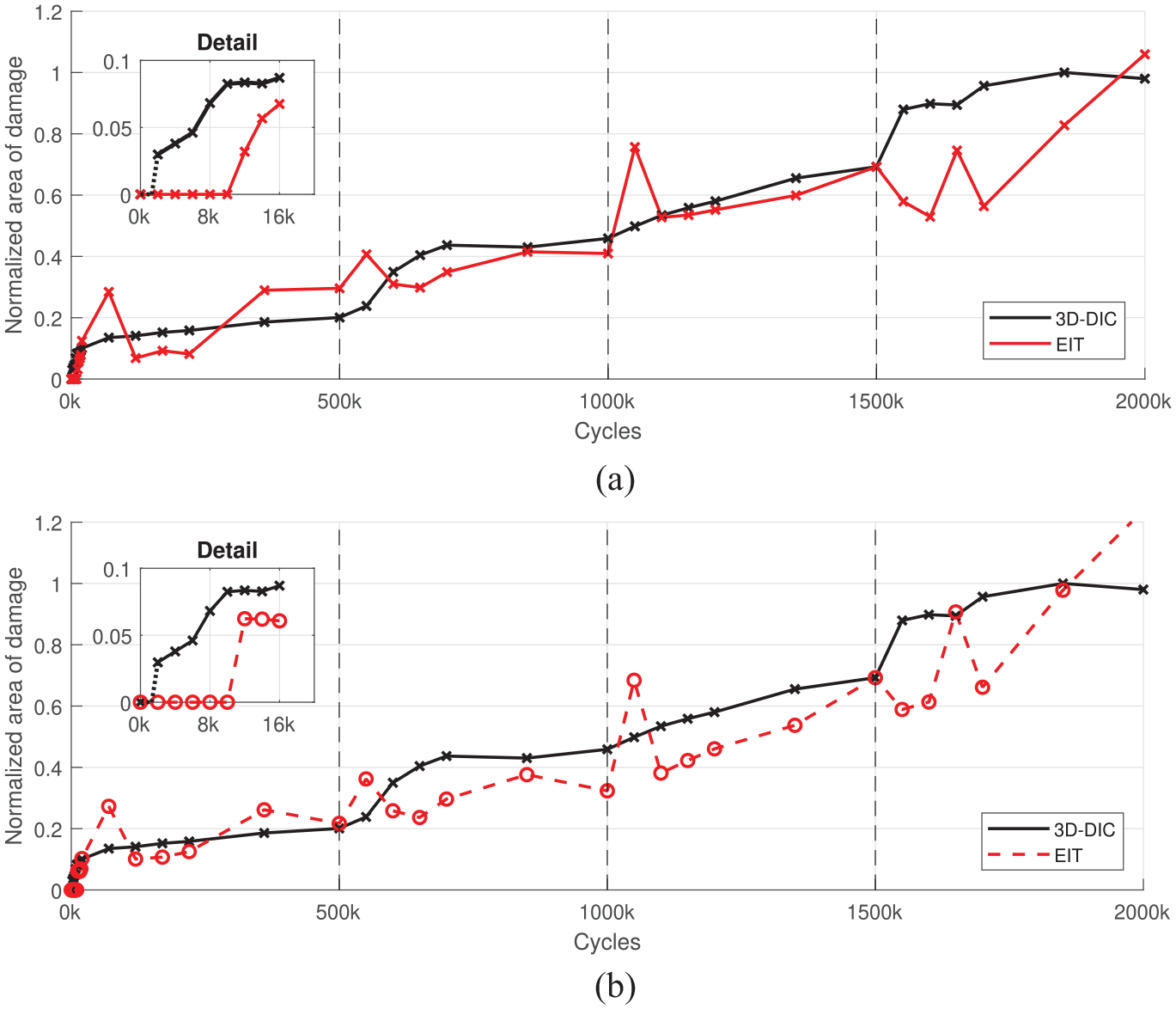
3D-DIC-based validation of EIT-based damage evaluation using continuous reference adjustment for (a) S_base,i to S_max,i and (b) S_base,i to S_mean,i.

It can be seen that the propagation of the damage-affected area evaluated by EIT qualitatively correlate with the results from the 3D-DIC. However, some noticeable differences are apparent. Existing differences, as given in Figure 15, are attributable to certain aspects. Particular, the discrepancies may be explained by the fact that the spatial conductivity changes are derived from measurements at different load levels, which gives a combination of mechanical loading and potential damage. Likewise, the applied primer, on which the thin-film sensor has been deposited, may additionally blur the strains, and local changes within the spatial strain field, which are not detected by the EIT reconstruction, might also induce such differences. A further aspect is the choice of the conductivity change thresholds for damage detection. Although a reduction of these threshold values improved the sensitivity, it also led to a significantly higher noise detection. Therefore, the choice provided the best trade-off between accuracy and robustness.

All these aspects are also reflected in the first proposed approach, except the evaluation at different load levels. However, as shown in Figure 14, the differences between 3D-DIC and EIT reconstructions are considerably smaller, indicating that these aspects may have a minor contribution to the observed differences, as can be seen in Figure 15. Consequently, the evaluation at different loads levels and the use of an updated baseline measurement S_base,i is likely to have a more significant contribution to the differences.

Compared to the first proposed approach, the agreement of the second proposed approach with the results of the 3D-DIC is weaker. However, the second approach could compensate a potential inhomogeneous “Set-In” effect (or inhomogeneous temperature and moisture distributions). This is particularly advantageous for significantly enlarged sensors (e.g., for application on complete shell-shaped structures) in the case that inhomogeneity is present. In the absence of any inhomogeneity related to the “Set-In” effect, the first proposed approach could also be used for significantly larger sensors.

Nevertheless, both proposed approaches demonstrate that progressive damage can be evaluated. While the 3D-DIC evaluates the entire evaluation area, the EIT uses voltage measurements at the boundary to reconstruct the electrical conductivity within the thin-film sensor. Consequently, the resulting resolution of the EIT reconstructions is smaller. Both methods rely on local changes within the evaluated area. It is likely that strain changes due to delaminations and micro-cracks caused by cyclic loading are responsible for the detected local changes. Using 3D-DIC, the delaminations and micro-cracks result in changes to the subsets (change of the gray value) and hence allow an evaluation, as the correlation coefficient passes the defined threshold value. Within the EIT reconstructions, delaminations and micro-cracks deteriorate the local conductivity, allowing an evaluation. However, no clear conclusion can be given whether the changes in conductivity appearing in the EIT reconstructions are caused by micro-cracks or by a relocation of the stress concentration (local “Set-In” effect at the stress concentration). Post-experiment inspection of the hole with a microscope does not show any detectable micro-cracks. Likewise, obvious damage to the sensor (e.g., chipping of the conductive sensor) can be excluded. Thus, a clear conclusion about the cause of the change in conductivity is not possible. Irrespective of this, the comparison with the 3D-DIC data demonstrates that the measured conductivity change corresponds to the damage growth obtained with 3D-DIC. Despite the fact that opposite sides (3D-DIC on backside, EIT on frontside) are evaluated, it is assumed that the occurring damage is reflected identically on both sides.

In common, to enhance the findings through EIT reconstructions and to obtain better agreement between EIT and 3D-DIC, the following considerations can be included. During the experiment, a single EIT measurement was performed at each load level. Several EIT measurements offer a possibility to identify potential outliers and the possibility of averaging the reconstructed spatial conductivity changes. In addition, a reduction in the size of the thin-film sensor or additional electrodes could be considered for improved spatial resolution. Both of these aspects would ensure that more information for the spatial reconstruction is available and, as a result, a more accurate evaluation could be carried out. Furthermore, a higher order reconstruction approach could be used like, for example, the generic algorithm according to Hassan and Tallman.²⁹

Similarly, adapting the hyperparameter can be taken into account in order to improve the agreement between EIT and 3D-DIC. Particularly considering Figure 14, it is expected that an adaptation would achieve an improvement beyond 1500k cycles. However, adapting the hyperparameter significantly increases the complexity of the evaluation algorithm, for example, the detection of the damage size must also be adapted to the hyperparameter.

Additionally, for the second proposed approach, a load independent analysis may be possible to compensate the mechanical loading component in the spatial conductivity change, so that only potential damage remains as a quantity. This may be achieved by a profound analysis of the elastoresistive properties and its dependency on fatigue loading. However, this is left for future research.

Conclusions

The present study demonstrates the potential of the EIT method featuring a spatial elastoresistive thin-film sensor for the monitoring of damage initiation and propagation in a cyclic-fatigue-loaded thin plain-woven CFRP component. As a case study, a CFRP plate with a centrally placed circular hole, that is subjected to high-cyclic tensile–tensile loading, is used. The applied strains were between 3000 and 12,000 μm/m and, thus, well represent a realistic operational loading of CFRP components, leading to realistic damage. The observed damage is a multiple delamination in combination with micro-cracks that initiates and propagates at both sides of the hole. For validation of the EIT results, a 3D-DIC system is used to monitor the shape and size of the damage. The electrical contacts at the used thin-film sensor did not show any visible deterioration. However, the thin-film sensor material showed a strong “Set-In” effect, followed by very constant electrical properties until it seemed to increasingly deteriorate over 1500k cycles. Consequently, the sensor network is concluded to be applicable for the monitoring of operational fatigue loading. Nevertheless, it is required to compensate this “Set-In” effect for fatigue and, therefore, realistic operational loading regimes. Two compensation approaches are proposed in the present article. The first uses a conductivity mean value adaptation and provides a very good correlation with the damage propagation identified by the 3D-DIC system. The second approach also demonstrates potential to monitor damage propagation by EIT; however, the superimposition of mechanical loads and potential damage corrupts the correlation.

Due to the nature of the used EIT reconstruction algorithm, the true shape of the damage cannot be identified and, thus, also not directly correlated with the 3D-DIC results. For the evaluation, if a damage at a location is present or not, a threshold is used. The damage propagation is observed by the summation of these damage-affected local areas. The damage locations identified by the EIT approaches perfectly match the 3D-DIC results. Furthermore, it is highly expected that more advanced reconstruction algorithms also enable the evaluation of the damage shape.

Future research shall address the characterization of the influence of the fatigue loading on the sensor material’s elastoresistivity and, furthermore, the identification of the true damage shape and the full spatial strain state by more advance EIT reconstruction algorithms to enable a better evaluation of the damage within the composite layup and its effect on the integrity of the structural component.

Nevertheless, it has been demonstrated within this paper that both proposed EIT approaches, which compensate EIT-related issues, can be used to describe damage progression originating from a circular hole due to cyclic fatigue loading at multiple loading levels. Consequently, the use of thin-film sensors offers a complementary method, with which damage propagation of thin plain-woven CFRP laminates with a circular hole could be evaluated.

Footnotes

Acknowledgements

The authors are grateful to Alexander Schöfer for his technical support during the experimental investigations.

Declaration of conflicting interests

The author(s) declared no potential conflicts of interest with respect to the research, authorship, and/or publication of this article.

Funding

The author(s) received no financial support for the research, authorship, and/or publication of this article.

ORCID iDs

Lukas Heinzlmeier

Christoph Kralovec

Martin Schagerl

References

Diamanti

Soutis

Structural health monitoring techniques for aircraft composite structures. Prog Aerosp Sci 2010; 46: 342–352.

Giurgiutiu

Structural health monitoring of aerospace composites, Cambridge, Massachusetts: Academic Press, 2016.

Niu

MCY

. Composite airframe structures: practical design information and data, Hong Kong: Conmilit Press, 1992.

Vassilopoulos

Keller

Fatigue of fiber-reinforced composites, 2013.

Nonn

Effects of defects and damage localization in carbon fiber reinforced polymer lightweight structures of aircraft composite structures. Rec Adv Appl Sens 2018; 15:1–110.

Australian Transport Safety Bureau. Fibre composite aircraft capability and safety. Aviation Research and Analysis Report AR-2007-21, ATSB, Australia, 2008.

Long

AC.

Design and manufacture of textile composites, 2005.

Flower

Soutis

Materials for airframes. Aeronaut J 2003; 107: 331–341.

Staszewski

Boller

Tomlinson

GR.

Health monitoring of aerospace structures: smart sensor technologies and signal processing. Hoboken, New Jersey: John Wiley & Sons, Ltd, 2004.

10.

Dalkilic

Improving aircraft safety and reliability by aircraft maintenance technician training. Eng Fail Anal 2017; 85: 687–694.

11.

Speckmann

Henrich

Structural health monitoring (SHM) overview on technologies under development. In Proceedings of the 16th world conference on NDT, 2017, vol. 1.

12.

Dienel

Meyer

Werwer

, et al. Estimation of airframe weight reduction by integration of piezoelectric and guided wave–based structural health monitoring. Struct Health Monit 2019; 18: 1778–1788.

13.

Dong

Kim

NH.

Cost-effectiveness of structural health monitoring in fuselage maintenance of the civil aviation industry. Aerospace 2018; 5: 87.

14.

Zhao

Gao

Zhang

, et al. Active health monitoring of an aircraft wing with embedded piezoelectric sensor/actuator. Smart Mater Struct 2007; 16(4): 1208.

15.

Soleimanpour

C-T

Wang

CH.

Higher harmonic generation of guided waves at delaminations in laminated composite beams. Struct Health Monit 2017; 16(4): 400–417.

16.

Di Sante

. Fibre optic sensors for structural health monitoring of aircraft composite structures: recent advances and applications. Sensors 2015; 15: 18666–18713.

17.

Katsikeros

Labeas

GN.

Development and validation of a strain-based structural health monitoring system. Mech Syst Signal Process 2009; 23(2): 372–383.

18.

Andraju

Raju

Damage characterization of CFRP laminates using acoustic emission and digital image correlation: clustering, damage identification and classification. Eng Fract Mech 2023; 227(4): 108993

19.

Cai

Qiu

Yuan

, et al. Structural health monitoring for composite materials. Compos Ther Appl, IntechOpen, Rijeka, Croatia, 2012: 1(3): 37–60.

20.

Makoond

Pelá

Molins

, et al. Automated data analysis for static structural health monitoring of masonry heritage structure. Struct Control Health Monit 2020; 27: e2581.

21.

Feng

MQ.

Computer vision for SHM of civil infrastructure: from dynamic response measurement to damage detection – a review. Eng Struct 2018; 156: 105–117

22.

Nonn

Schagerl

Zhao

, et al. Application of electrical impedance tomography to an anisotropic carbon fiber-reinforced polymer composite laminate for damage localization. Compos Sci Technol 2018; 160: 231–236.

23.

Cagáň

Pelant

Kyncl

, et al. Damage detection in carbon fiberrein–forced polymer composite via electrical resistance tomography with Gaussian anisotropic regularization. Struct Health Monit 2019; 18: 1698–1710.

24.

Loyola

Saponara

Loh

, et al. Spatial sensing using electrical impedance tomography. IEEE Sens J 2013; 13: 2357–2367.

25.

Rocha

Fernandes

Ferreira

, et al. Damage localization on CFRP composites by electrical impedance tomography. Mater Today Commun 2022; 32: 104164.

26.

Baltopoulos

Polydorides

Pambaguian

, et al. (2013) Damage identification in carbon fiber reinforced polymer plates using electrical resistance tomography mapping. J Compos Mater 2013; 47: 285–301.

27.

Tallman

Gungor

Koo

, et al. On the inverse determination of displacements, strains, and stresses in a carbon nanofiber/polyurethane nanocomposite from conductivity data obtained via electrical impedance tomography. J Intell Mater Syst Struct 2017; 28: 2617–2629.

28.

Loh

Hou

Lynch

JP.

Carbon nanotube sensing skins for spatial strain and impact damage identification. J Nondestr Eval 2009; 28: 9–25.

29.

Hassan

Tallman

Failure prediction in self-sensing nanocomposites via genetic algorithm-enabled piezoresistive inversion. Struct Health Monit 2020; 19: 765–780.

30.

Enser

Sell

Hilber

, et al. Printed strain sensors in organic coatings: in depth analysis of sensor signal effects. Sens Actuators A Phys 2018; 2: 258–263.

31.

Wagner

Kralovec

Kimpfbeck

, et al. Framework for strain measurements at cyclic loaded structures with planar elastoresistive sensors applying electrical impedance tomography. Eur Workshop Struct Health Monit 2023; 253: 805–815.

32.

Wagner

Gschoßmann

Schagerl

On the capability of measuring actual strain values with electrical impedance tomography using planar silkscreen printed elastoresistive sensors. IEEE Sens J 2021; 21: 5798–5808.

33.

Gschoßmann

Zhao

Schagerl

Development of data acquisition devices for electrical impedance tomography of composite materials. In Proceedings of the 17th European conference on composite materials (ECCM17), MAI Carbon Cluster Management, Augsburg, Germany, 2016. pp. 1–8.

34.

Heinzlmeier

Sieberer

Kralovec

, et al. Fatigue and progressive damage of thin woven CFRP plates weakened by circular holes. Exp Mech 2023; 63: 871–883.

35.

Correlated Solutions Inc. VIC-2D reference manual – knowledgebase – manuals and guides, https://correlated.kayako.com/section/9-manuals-and-guides (2023, acces-sed 9 August 2023)

36.

Correlated Solutions Inc. VIC-3D manual and testing guide – knowledgebase – manuals and guides, https://correlated.kayako.com/article/57-vic-3d-8–manual-and-testing-guide (2023, accessed 9 August 2023)

37.

Sutton

Orteu

J-J

Schreier

Image correlation for shape, motion and deformation measurements. New York, NY: Springer, 2009.

38.

Daly

SH.

Digital image correlation in experimental mechanics for aerospace materials and structures. In Encyclopedia of Aerospace Engineering. Hoboken, New Jersey: John Wiley & Sons, Ltd, 2010, no. 1, pp. 1–2.

39.

Murray

Kalteremidou

Carrella-Payan

, et al. Failure characterisation of CF/epoxy V-shape components using digital image correlation and acoustic emission analyses. Compos Struct 2020; 236: 111797.

40.

Rogani

Navarro

Marguet

, et al. Study of post-impact behaviour of thin carbon/epoxy laminates subject to fatigue tensile loading. Int J Fatigue 2021; 148: 106134.

41.

Heinzlmeier

Sieberer

Wolfsgruber

, et al. Damage propagation and residual strength of simple block-loaded CFRP plates with circular holes under tension–tension fatigue conditions. J Compos Sci 2023; 7(9): 379.

42.

Adler

Guardo

Electrical impedance tomography: regularized imaging and contrast detection. IEEE Trans Med Imaging 1996; 15: 170–179.

43.

Adler

Dai

Lionheart

WRB

. Temporal image reconstruction in electrical impedance tomography. Physiol Meas 2007; 28: S1–S11.

44.

Cheney

Isaacson

Newell

, et al. Noser: an algorithm for solving the inverse conductivity problem. Int J Imaging Syst Technol 1990; 2: 66–75.

45.

dos Santos

CAM

de Campos

da Luz

, et al. Procedure for measuring electrical resistivity of anisotropic materials: a revision of the Montgomery method. J Appl Phys 2011; 110: 66–75.

Damage evaluation in plain-woven CFRP plate with circular hole under cyclic tensile loading using electrical impedance tomography

Abstract

Keywords

Introduction

Material and methods

Specimen

Experimental procedure

Damage evaluation by DIC (3D-DIC)

Damage evaluation by EIT

Results

3D-DIC damage evaluation results

EIT-based fatigue damage evaluation results

Discussion

Conclusions

Footnotes

Acknowledgements

Declaration of conflicting interests

Funding

ORCID iDs

References