
Abstract
In population-based structural health monitoring, the aim is to make inferences about the health of structures using information from a population of other structures. It is possible to use transfer learning here, as long as the structures that are used for transfer behave similarly to each other. As a result, assessing the similarity of structures and the data collected from those structures is necessary for successful transfer. In this paper, ideas from kernel and graph theories are used to assess whether the constructional makeup of two engineering structures – a bridge and a wind turbine, for example – are similar or not. To the human brain, this notion may seem trivial because the intended use, construction and behaviours of these structures are vastly different. However, for a computer, automatically measuring these dissimilarities requires a whole host of information. In this paper, the aim is to use irreducible-element models and attributed graphs to represent engineering structures, and to use graph kernels to measure the similarity of these models. The proposed methods are able to compare discrete and continuous attributes of structures in polynomial time. Similarity assessments are provided for a group of toy structures as well as a case study of seven real operational bridges. The latter population is important in dealing with a class of highly complex real-world examples of civil infrastructure; the analysis also allows a discussion on which aspects of bridge construction might be responsible for structural similarity or dissimilarity.
Introduction
Structural health monitoring (SHM) aims to continuously monitor structures throughout their lifetime in order to detect, localize, quantify and predict damage. 1 In particular, data-based SHM methods focus on collecting data from sensor networks installed on structures and utilizing them within machine learning models in order to make inferences about their health. One of the biggest challenges of SHM, however, is the availability of informative data. Specifically, labelled data pertaining to damage are difficult and expensive to obtain. As a result, developing SHM methods that capture all possible damage scenarios that a typical structure may undergo is extremely challenging. A proposed solution to this major drawback of SHM is population-based SHM (PBSHM).2–8 The main motivation for the framework is to allow data from one structure to strengthen health-state inferences on a different one, that is, to make inferences about the health of structures for which there may be little to no damage-state data, by studying structures that exhibit damage information. The populations of structures in question can be homogeneous – where the structures are nominally identical – or heterogeneous, where the structures can be different to each other. The PBSHM methodology can, therefore, increase the pool of information available to make diagnostic and prognostic decisions.
The main means of allowing such cross-structure diagnostics is via the machine learning discipline of transfer learning,9,10 which transfers knowledge from source domains to target domains. In PBSHM, the source domain contains labelled data from structures, whereas the target domain contains data from structures for which there is a lack of labelled data. The aim of transfer learning is to develop models in the source domain that generalize well to the target domain. Transfer learning has been applied successfully in PBSHM in numerous studies to make inferences about health of structures. For example, transfer component analysis was undertaken to identify damage on a tail-plane by studying a population of tail-planes. 11 Domain adaptation (a form of transfer learning), combined with Gaussian mixture models, was used to transfer damage-state information across two bridges that made up a heterogeneous population. 12 Transfer learning has also helped address the problem of repair 13 ; structural repairs can cause the underlying distribution of the data to shift, causing significant discrepancies between training and testing data. Domain adaptation can minimize these shifts and improve the performance of machine learning models. A significant issue in transfer learning is that attempted transfer between wildly disparate structures will make matters worse. Therefore, one main takeaway from these studies is that the similarity of the data in the source and target domains is an important consideration, because dissimilarity can increase the threat of negative transfer. Negative transfer takes place when the performance in the target domain is adversely affected by transferring information from the source domain. Interestingly, structural similarity (as well as similarity between features extracted from the collected data) also plays a significant role in reducing the threat of negative transfer in PBSHM. 14 The hypothesis in PBSHM is that feature data collected from structures are best suited for transfer learning if the structures (from which the data were collected) are also similar.
As mentioned, a hypothesis of PBSHM is that similarity of structures is a necessary condition for transfer of inferences. These inferences could be of multiple forms; in the first place, one might wish to transfer a classification task – like damage localization – as illustrated in Gardner et al. 14 Another possibility for transfer is a decision process, where one is considering a risk-based approach to SHM, as in Hughes et al.15,16 Regarding the strength of the hypothesis itself, recent work has shown a strong predictive relationship between structural similarity measures and the likelihood of positive transfer. 17
To assess the similarity of feature data, distance metrics can be utilized; distance metrics are non-negative
In order to deal with this issue, PBSHM is based on an abstract representation of structures, in which structures become points in a metric space. The ‘metric’ aspect of the space is crucial; it allows a measure of distance, or similarity, between structures such that transfer should only be attempted between those which are ‘sufficiently close’. The abstract representations of the structures are in the form of irreducible element (IE) models or attributed graphs (AGs) 3 in this paper. An IE model can be used to represent a structure by separating it into meaningful components that have well-established dynamic behaviours. It is then possible to include information such as the geometry, topology and material properties of these components, by forming an AG. Both of these representations can also incorporate information about the joints that connect the elements together.
At this point, it may be helpful to formulate this problem as a fibre-bundle (Figure 1), as introduced by Tsialiamanis et al.
20
The aim of the fibre-bundle in PBSHM is to bring together information about the composition of the structures – in terms of AGs
3
– and their associated sensor data as features. The concept can be broken down into three spaces; the space of AGs
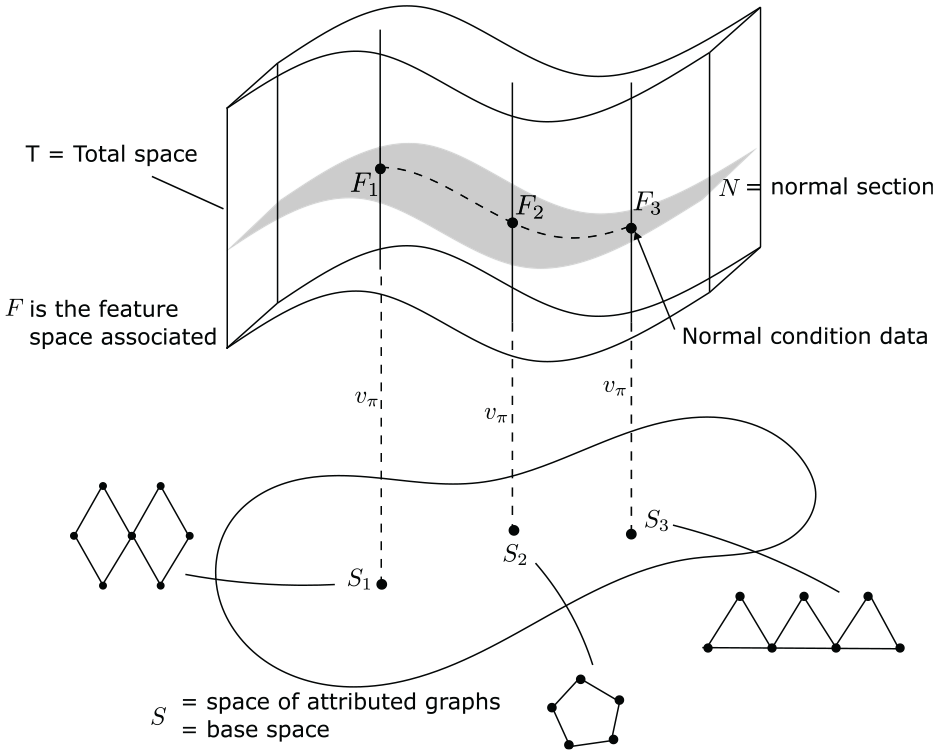
Schematic of a fibre-bundle showing the spaces of structures and features in PBSHM.
The idea of transfer across heterogeneous populations raises the question of when structures or substructures are sufficiently similar that transfer is possible, that is, does not lead to negative transfer, and make diagnostics worse. Within the fibre bundle, there may be some target structure
Successful topological comparisons were conducted using AGs to form communities of similar structures for transfer in the context of PBSHM. 21 However, the method based on the Jaccard distance 21 can only compare discrete attributes within the graphs, that is, whether the two attributes being compared are the same or different. Moreover, the described method leads to a high computational burden. The current paper aims to extend these capabilities to include comparison of continuous node attributes by applying kernel-based methods. This is a significant, and indeed a necessary, extension to the current framework, because the ability to compare continuous node labels such as material properties is crucial to comparing structural behaviours in PBSHM. 22 The graph-kernel methods used in this paper are based on previous work on protein function prediction in the field of biology,23–28 where graphs with continuous and discrete attributes are compared in polynomial time.
In this paper, the graph-kernel approach to assessing similarity of structures will first be applied to a toy dataset. The toy dataset was introduced by Gosliga et al. 21 to demonstrate a method of measuring the topological similarity between structures using discrete node labels. The same toy dataset is used in this paper to illustrate the benefit of implementing graph kernels – where the comparison can be extended to continuous node labels – while significantly reducing the computational time required. Here, the complexity of included labels in the formulation is systematically increased. The most suitable developed methodology is then applied to a population of real operational bridges in order to form similar communities for transfer learning.
Original contribution
This is the first scientific study on developing a framework for measuring similarity between graphical representation of structures for PBSHM that extends beyond discrete node-label comparison to continuous node labels. This methodology takes the next step in assessing structures in a metric space to find similar structures for transfer. By using graph kernels, populations of structures can be compared quickly and effectively. A number of graph kernels ranging from those that compare discrete node labels to more sophisticated kernels that compare continuous labels are applied to find the most suitable solution. The advantages and drawbacks of these kernels are discussed in the context of PBSHM. The developed methods are applied to two datasets. The first dataset contains a population of toy structures that demonstrates the effectiveness of these techniques in a truly heterogeneous population. The second is a population of real bridges represented by much larger graphs (in comparison to the toy structures) that illustrates the success of applying graph kernels to form communities of similar structures and the computational efficiency of the proposed methods.
The structure of the paper is as follows. In section ‘Graphical representation of engineering structures’, the abstract representation of structures in the form of IEs and AGs is explained. The toy dataset used in the first part of this paper is then described in section ‘The toy dataset’. In section ‘Related work on assessing similarity of graphs for PBSHM’, previous work on comparison between structures for PBSHM is presented to demonstrate the current state of research in this topic. Section ‘Graph kernels’ then introduces graph kernels and presents the results of applying graph kernels to the toy dataset. A case study is then conducted in ‘Case study: Measuring the similarity between a heterogeneous population of bridges’ section where the most suitable graph kernels from section ‘Graph kernels’ are applied to a population of operational bridges. Finally, section ‘Conclusions and future work’ includes the conclusions and future work.
Graphical representation of engineering structures
The first stage in establishing the representation of a structure for similarity assessment is to construct an IE model. 3 An IE model of a structure is intended to capture the essential nature of that structure in terms of a small (if possible), set of fundamental structural elements of well-established dynamic behaviours. These elements can be labelled as fundamental engineering objects, for example, beam, plate, shell, etc., or contextually, for example, wing, deck, blade.
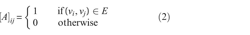
The second step in representation is to convert the IE model into an AG. In the AG representation, individual IEs appear as nodes (vertices) in the graph, while the information about how elements join together is encoded in graph edges. Each node and edge is assigned a vector of attributes, which specify details such as type, material and geometry, etc. The important point now is that the space of AGs is a metric space, as mentioned above. Details of how IEs and AGs are formed are explained by Gosliga et al., 3 along with an example of a metric on the space of graphs.
The level of resolution one may include in these models is subjective. For example, there is no standard for determining the separation method for a wind-turbine tower section or deciding the breakdown of components in aeroplane landing gear. In this paper, engineering judgement is used to represent the structures using the most logical elements. An in-depth study on this topic has been conducted for PBSHM by Brennan et al. 29
Once the structures are in the form of IEs and AGs, graph theory can be used to analyse them. A graph

For comparison, similarly, a second graph can be expressed as
where
Following the conversion of structures to abstract graphical representations, similarity between graphs can be measured. In the next section, the toy dataset used by Gosliga et al. 25 is presented to evaluate the techniques developed in this paper.
The toy dataset
To test the suitability and effectiveness of graph kernels for PBSHM, the dataset introduced by Gosliga et al. 21 is used in this paper. The dataset consists of six simplified, common engineering structures with varying topology, geometry and material compositions, allowing the use of kernels for assessing similarity between discrete and continuous node labels. Figure 2 presents these labelled structures (a wind turbine, two aeroplanes and three bridges), alongside their graphical representations.
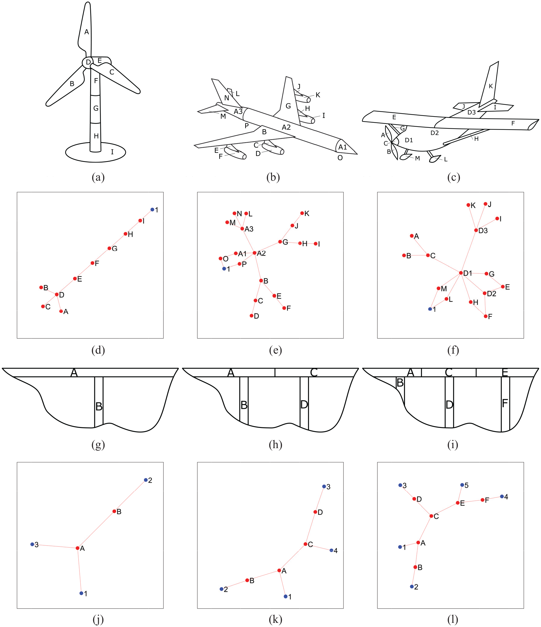
The structures in the dataset, and the corresponding graphs, with nodes labelled according to elements. Each red node represents an irreducible element from the original structure. These nodes are associated with information, such as the geometry of the element and its material properties. The blue nodes are ground nodes that can control boundary conditions. These graphs can be used to compare the topological similarity of the structures. The structures (a) Turbine 1, (b) Aeroplane 1, and (c) Aeroplane 2, and the corresponding graphs (d) Turbine 1, (e) Aeroplane 1, and (f) Aeroplane 2. The structures (g) Bridge 1, (h) Bridge 2, and (i) Bridge 3, with the corresponding graphs (j) Bridge 1, (k) Bridge 2, and (l) Bridge 3.
In this paper, the focus is on measuring the similarity when considering the node labels (specifically, the material properties, geometry and element types), of each graph. Here, the density, tensile strength, modulus of elasticity and the coefficient of thermal expansion are used as the material properties. The geometry of the element is represented by its total volume. The elements that make up the structures are assigned a type according to shapes with well-defined dynamical behaviours when possible. Here, ‘beams’, ‘shells’ and ‘plates’ are used for components such as towers on turbines, engine casings on aeroplanes and decks on bridges. Additionally, some elements are assigned the type ‘complex’ when the aforementioned types are unsuitable; landing gear and rotor hubs fall into this category. Finally, there exist ‘ground’ nodes; these are connected to elements that contact the ground or their surrounding environment. These nodes are highlighted in blue in Figure 2, and their adjacent edges control boundary conditions. For simplicity, boundary and edge attributes are not considered here for similarity comparisons.
Figure 3 visually presents the materials30–39 and types assigned to each element in the dataset. A specific combination of shapes and colours are used here to define the attributes. For example, a square node, coloured in green is a concrete beam, etc.
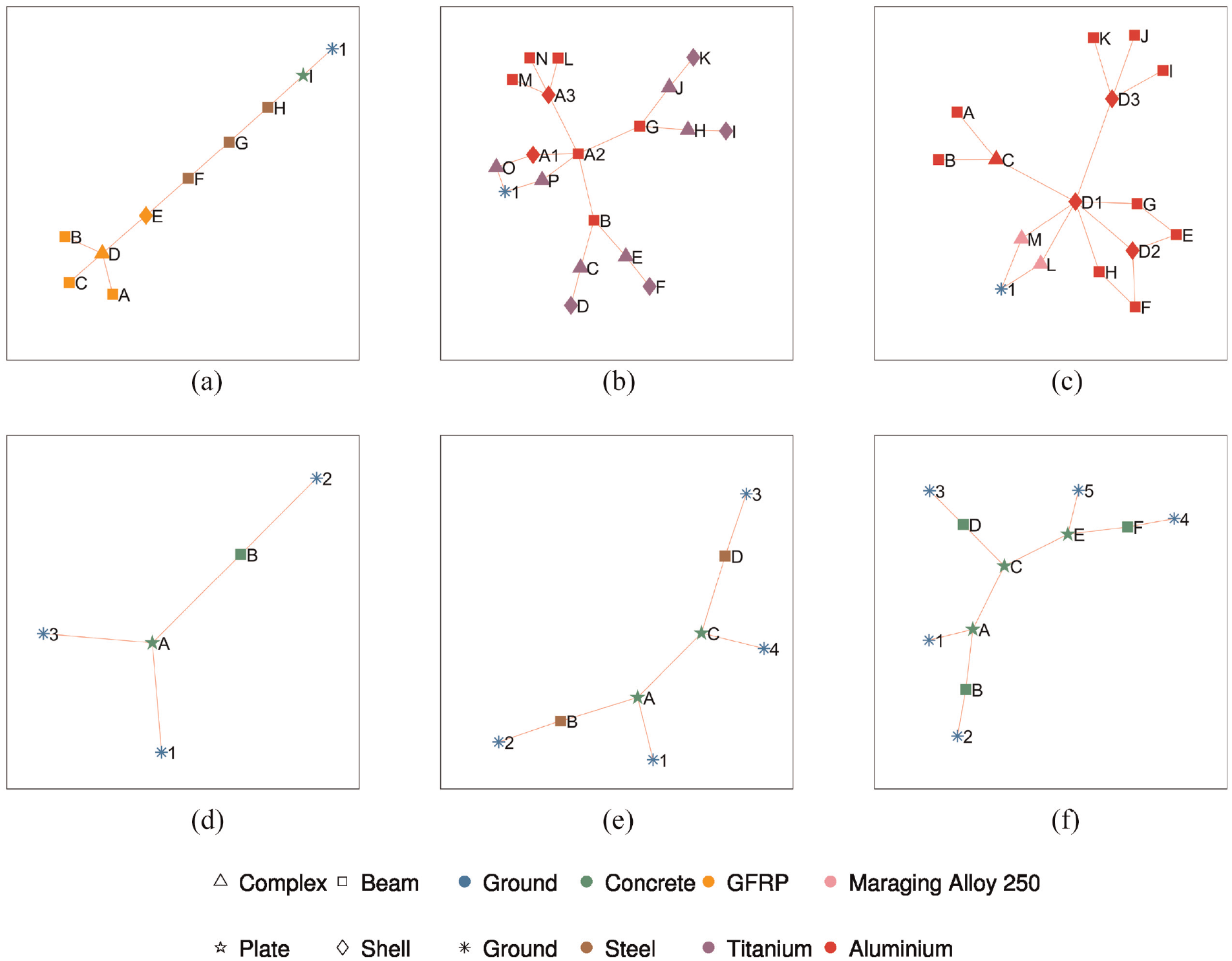
The graphs from Figure 2 re-imagined with element types (shape of the nodes) and materials (colour of the nodes) highlighted for visual comparison. (a) Turbine 1. (b) Aeroplane 1. (c) Aeroplane 2. (d) Bridge 1. (e) Bridge 2. (f) Bridge 3.
In the following section, previous related work that demonstrates the methods used in PBSHM for AG similarity assessment is presented. The described methods compare the topology and discrete node attributes, as well as structural equivalence using ideas from graph matching. Advantages and drawbacks of using such methods are also discussed.
Related work on assessing similarity of graphs for PBSHM
When it comes to measuring similarities between graphs, the idea of topology becomes a key component. The topology of structures can be established by the connections between nodes of graphs. A structure’s topology can help determine its dynamic behaviour; comparing topologies between structures enables insight into their dynamic similarities. Without obtaining any attributes about the elements, it is possible to compare two graphs simply by assessing their topology. By considering the isometry classes of metric spaces, distance metrics can be found between two graphs of different sizes. 40 Gromov-Hausdorff distance, the Kantorovich-Rubinstein distance and the Wasserstein distance are some of the example metrics that can be used in this case.
One should, however, consider structural equivalence rather than just topological similarity 22 for a stronger comparison between structures (i.e. the AGs should be directly equivalent with ground nodes in corresponding places 21 ). The current state of research in assessing structural similarity for PBSHM is, therefore, based on calculating the structural equivalence between graphs.21,41 By determining the maximum common subgraph (MCS) between two graphs – a common substructure in the structures of interest – it is possible to include structural equivalence. Previous work 21 used the modified Bron-Kerbosch algorithm to obtain the MCSs, which is the same process replicated in this work. A distance metric can then be used between the graphs of structures and their MCSs to obtain a measure of similarity. In related work by Gosliga et al.,21,41 the Jaccard similarity coefficient,
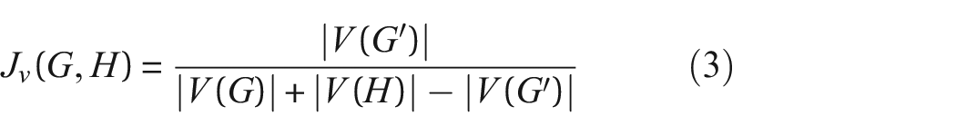
is utilized to obtain the Jaccard distance,

giving a measure of structural similarity. Here,
The Jaccard distance
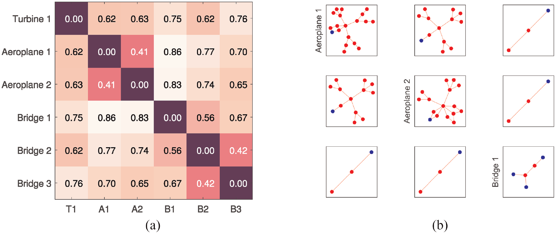
(a) The topological similarity between the structures and their MCSs, calculated using the Jaccard distance
At the next level of detail in comparing structures, one can consider other attributes, such as the material properties and geometry of the elements that provide a comprehensive characterization of the structures. This information is encoded in the AG representation via the node attributes. To aid comparison, a metric that is more sophisticated than the Jaccard distance is needed, because the Jaccard + MCS method is unable to process continuous node labels. In the next section, graph kernels are introduced as a method for assessing similarity between AGs.
Graph kernels
Graph kernels, introduced by Gärtner et al.
42
and Kashima et al.,
43
were designed as a similarity measure for comparing graph substructures that can be computed in polynomial-time. The aim was to find a mapping
In order to find the mapping
Graph kernels are convolution kernels on pairs of graphs and can be used in any kernel method, such as classification, clustering, etc. 46 Graph kernels in the RKHS are positive definite where a distance function can be defined as,

If

if and only if
Following Mercer’s theorem, the Gram matrix that represents the positive definite graph kernels can be normalized to obtain a scale-invariant similarity measure. 47 The Gram matrix or the graph kernel is normalized by
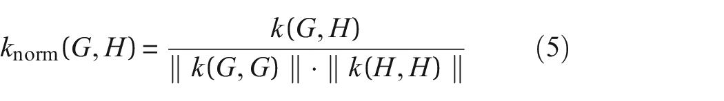
where the norm of a graph kernel calculated on
There exists many types of graph kernels; some are based on ‘walks’, 23 some on ‘paths’, 24 others on ‘graphlets’ 48 and ‘subtrees’, 49 to name a few. The strength of these kernels arise from the ability to compare, not only the substructure of graphs, but also their node attributes.
One of the fastest kernels capable of assessing large graphs with discrete node labels is the Weisfeiler-Lehman (WL) graph kernel. 49 This kernel can be used as a suitable first step to assess the similarity of IEs by comparing the topology of the elements, represented in the AGs as discrete node labels such as ‘beams’ or ‘shells’. In this paper, these node labels will be referred to as type labels henceforth.
WL graph kernel
The WL framework is an iterative algorithm that helps identify if two graphs are isomorphic. It is based on assessing the subtrees of two graphs to identify if the graph substructures are similar. The general idea here is to iteratively relabel graph substructures that differ until the the label sets of the two original graphs are completely different. The runtime complexity of the WL framework is
The WL kernel with
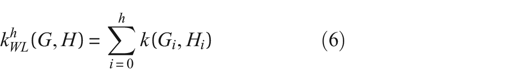
where

and
The new labels

where

which suggests that
The kernel values of each iteration are added to obtain the final kernel value. The Gram matrix normalization method discussed earlier is applied to obtain a measure of similarity across the entire population.
A visual example of the graph relabelling process is is presented in Figure 5(a) to (d). Here, Bridge 1 (referred to as graph
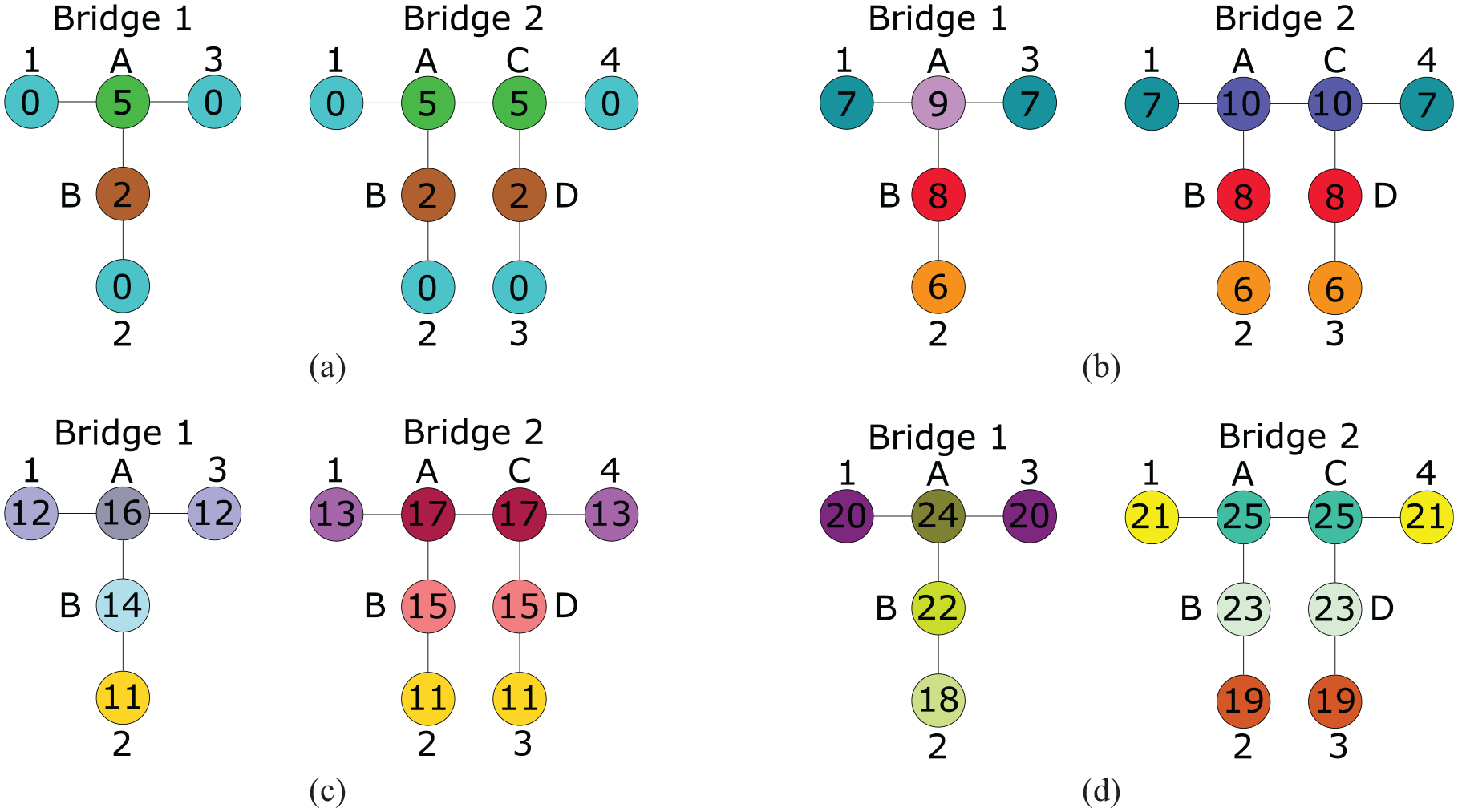
The evolution of node labels with each iteration of the WL-kernel when comparing data from Bridge 1
The neighbouring node labels
The node labels at each iteration of the WL kernel for Bridge 1
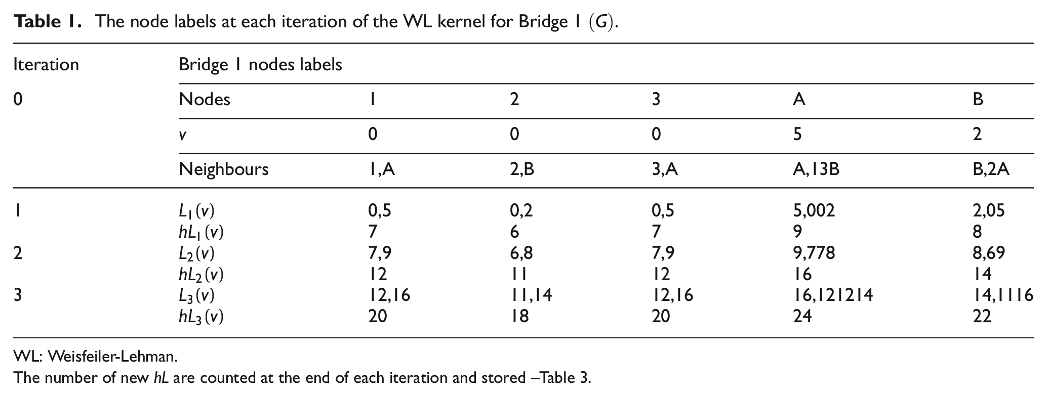
WL: Weisfeiler-Lehman.
The number of new
The node labels at each iteration of the WL kernel for Bridge 2
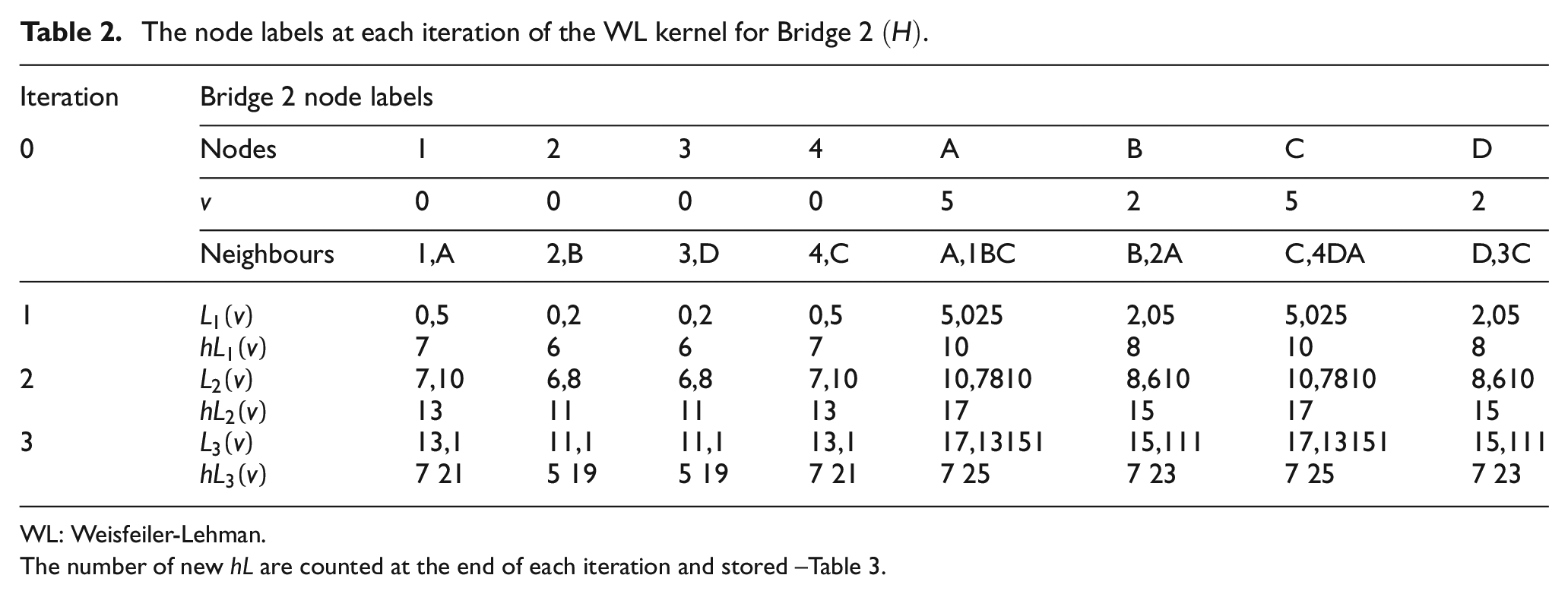
WL: Weisfeiler-Lehman.
The number of new
The counts of node labels of Bridge 1
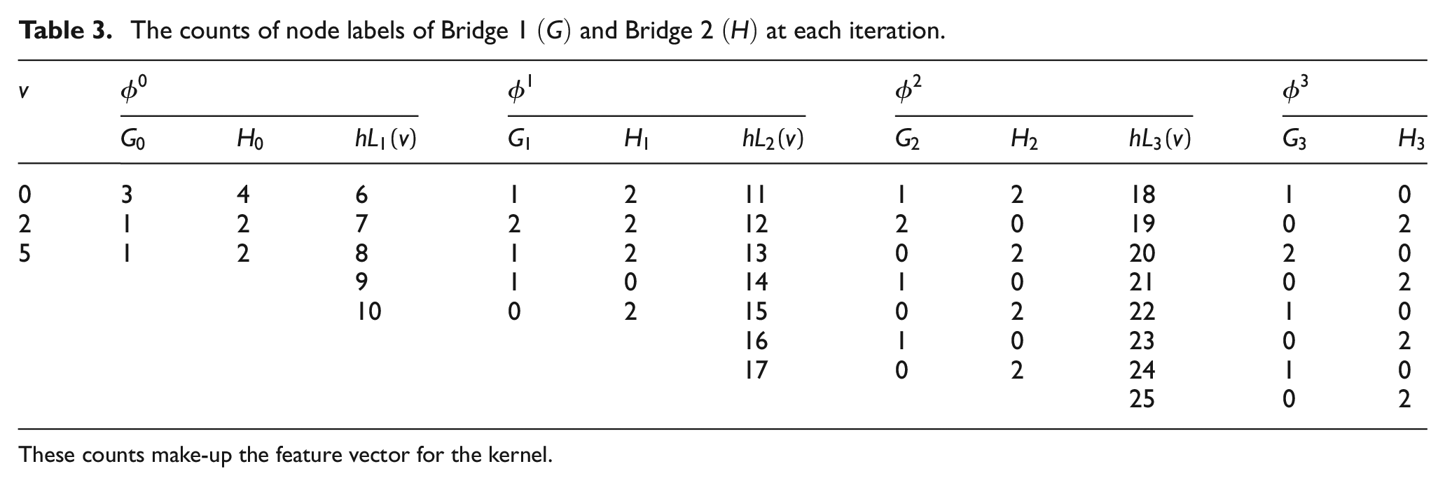
These counts make-up the feature vector for the kernel.
The similarity between the structures (introduced in section ‘The toy dataset’) calculated using the WL kernel is presented in Figure 6(a). Here, discrete node labels that describe element shapes are included in the formulation. Since the WL kernel only considers the labels of the neighbouring nodes in each graph, topological similarity is preserved here. Adding the information about the element types has grouped the three bridges together. This result is unsurprising as the bridges only contain a combination of beam and plate elements. Aeroplane 2 and Turbine 1 are constructed predominantly of beams, which may be the reason for their apparent high similarity. The similarity values calculated by the kernel when considering only the topology as well as the inclusion of type labels are found in Figure 6(b). As node labels are incorporated, the increase in distance between the structures is expected; the structures will move further apart in the metric space when more information – that describe the differences between them – is included.
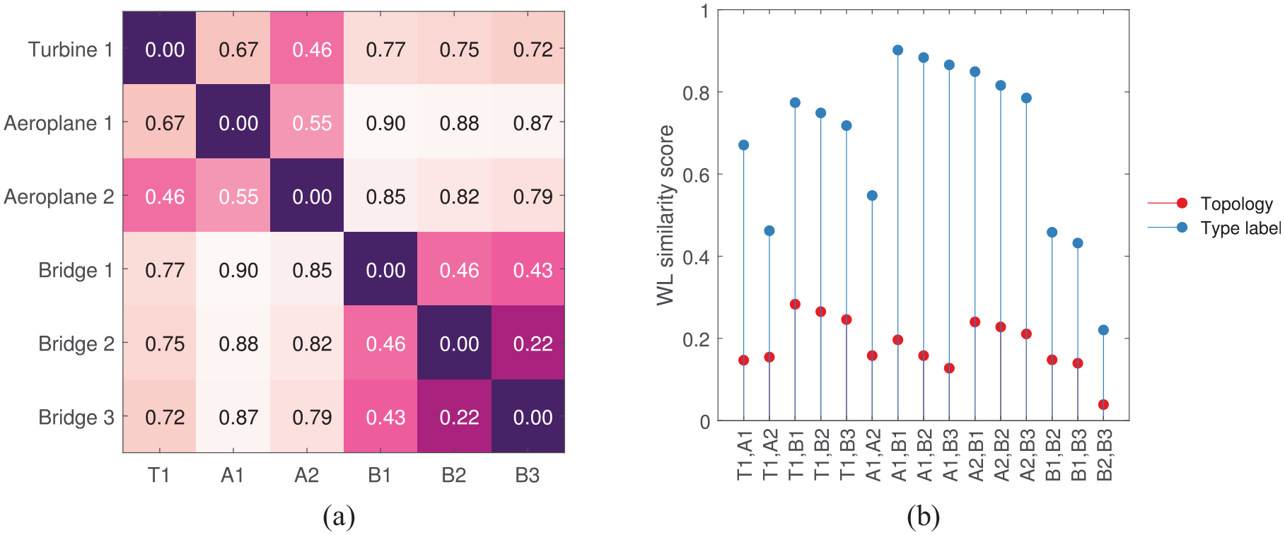
(a) The similarity of graphs from section ‘The toy dataset’ calculated using the WL kernel. Here, the discrete node labels that describe the shape of each element (as seen in Figure 3) are included in the kernel. (b) The kernel values when considering only topology (red) and when including type labels (blue).
The WL kernel is clearly a useful tool to find similarity of graphs with discrete node labels. Shervashidze et al. 49 suggest a faster algorithm that enables the global computation of multiple graphs simultaneously. The runtimes of large graphs are much faster when using the said global method compared to pairwise comparisons. As civil structures can comprise many elements, the global WL kernel may be very useful for PBSHM. This kernel is, however, not able to compare continuous node attributes that are included in AGs. In the next section, the random walk (RW) kernel is presented, that is capable of handling both discrete and continuous node attributes.
The RW kernel
In biology research, to compare different types of graph attributes in protein function prediction, the RW kernel was successfully utilized by Borgwardt et al. 23 The kernel is able to analyse both continuous and discrete node labels, providing many advantages over previous attempts, making it a powerful tool for attributed-graph comparison. The advantages stem from the fact that comparing discrete labels indicates whether two nodes are the same or not, whereas comparing continuous labels are helpful to obtain a sliding scale of similarity/dissimilarity. In the context of SHM, the ability to compare continuous node labels will be used to include material properties of each element of the structure into the kernel. Including discrete and continuous node labels can help assess the similarity of structures and obtain a full picture of the differences between structures in terms of their topology, geometry and material properties. Consequently, the RW kernel may help to verify the PBSHM framework established in ‘When is a bridge not an aeroplane?’ by Worden et al. 22 where the hypothesis is: distances – a measure of dissimilarity – between structures that are different will increase, as more information is added to the AGs (as attributes) that describe the structures.
In its simplest form, the RW kernel counts the number of matching labelled RWs within two graphs and provides a measure of topological similarity. Later, methods that include discrete and continuous attributes within the RW formulation are discussed. A ‘walk’ of length
The RW kernel is defined as,
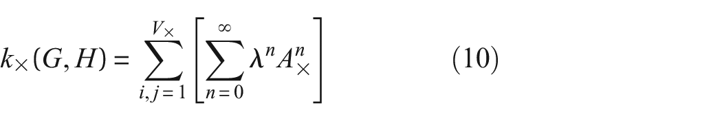
where
Equation (10) can be computed using the preconditioned conjugate-gradients method
50
(used here that computes in
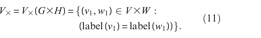
The RW kernel in Equation (10) can be modified to include a number of other positive-definite kernels operating on attributes, that is, kernels assessing discrete and continuous labels can, therefore, be included as part of the adjacency matrix. The adjacency matrix of the modified RW kernel from Equation (10) becomes,
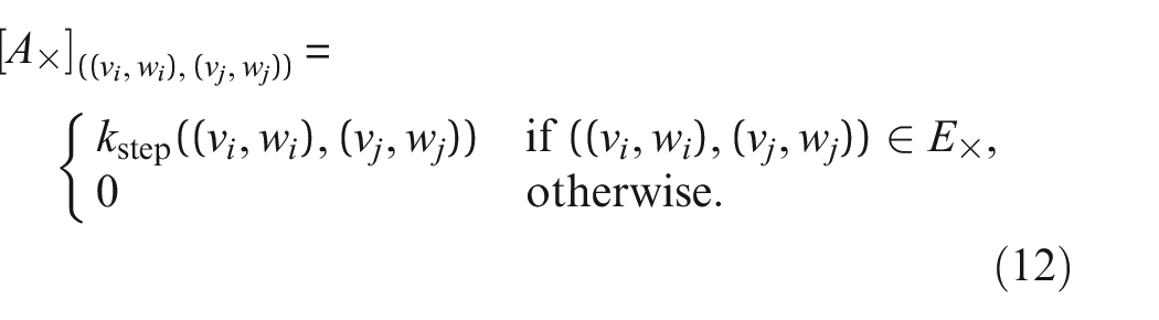
where
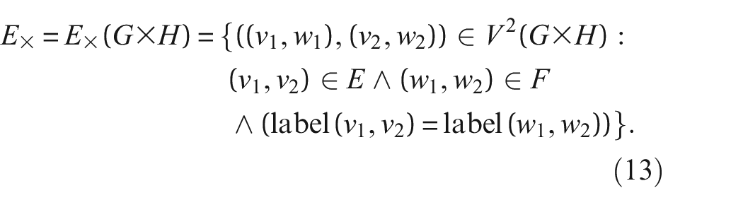
where ∧ is a logical AND operator.
The step kernel (not accounting for edge similarity) for
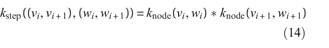
and the

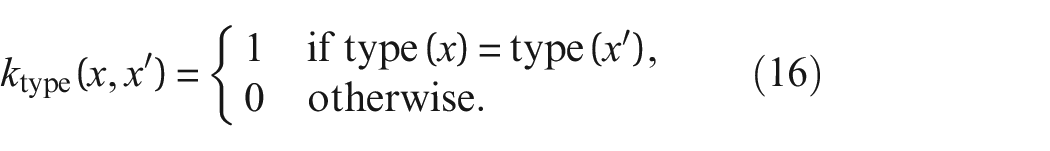
As suggested by Borgwardt et al., 23 a type kernel can assess discrete labels within the RW. In this work, discrete node labels that describe the shape of each element (e.g. ‘beam’) are designated type labels, and will be used within the type kernel. The type kernel only allows a walk in the direct product graph if the two nodes are the same type. For this step, a Dirac kernel is used, where a value of 1 is given if the two nodes are of the same type, and a 0 is given otherwise, that is,
For evaluating continuous attributes, a node-label kernel is employed here. The node-label kernel uses the Gaussian kernel to evaluate any vectorized continuous attributes. In this case, the material properties of the elements are used as the node labels. The Gaussian kernel is defined here as,
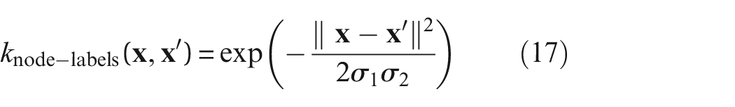
where
Once the RW kernels are calculated on each pair of graphs in the population, similarity measures are obtained by normalizing the Gram matrix. The similarity between the structures in the toy dataset when considering their type and material properties is presented in Figure 7(a). Slightly different types of concrete were used in the beams and plates for Bridge 2 and 3 in order to obtain non-zero node-label kernel values. By including these attributes, the RW kernel has identified high similarities within the group of bridges and within the two aeroplanes. This is a useful initial result for PBSHM, as likely candidates for positive transfer have been identified and grouped together. Interestingly, high similarities are observed between Turbine 1 and Bridge 2, which does not make physical sense. From Figure 7(b), the reason for this behaviour can be attributed to the similarities in the material properties as the kernel values are not pulled apart here. Both structures contain a combination of steel and concrete components, which may be the underlying reason for this result. This is possibly an artifact of comparing high-level similarities where little information is provided in the AGs. This result is expected to improve as more information is included in the formulation.
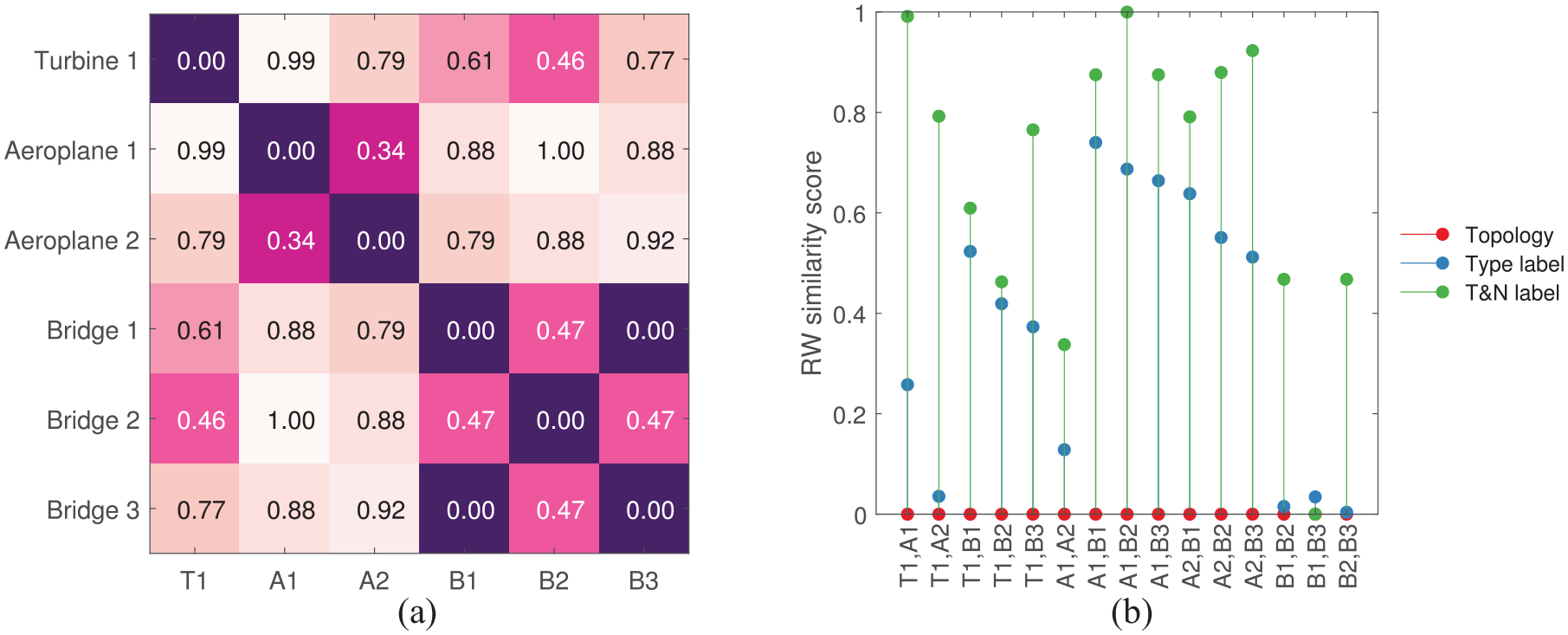
(a) The distance between graphs from section ‘The toy dataset’ calculated using the RW kernel. Here, the discrete and continuous node labels that describe the shape and material properties of each element are included in the kernel. (b) The kernel values when considering only topology (red) and when including type labels (blue) and material properties (green). Worden’s 22 hypothesis that distances will increase as more attributes are added to the AGs is verified in (b).
One must now take care when considering these structures for transfer, as an important attribute has been left out of formulation up to now, which is the dimensions of the elements. It should be obvious that even though the two aeroplanes are similar to one another when considering the current (rather crude) attributes and the RW kernel, that they are, in fact, considerably different in practice. In this specific context, the main difference in these structures arise from their size (if one is to make the assumption that their aspect ratios remain consistent). By employing the Brownian bridge kernel, 23 a length kernel,

can be introduced into Equation (15), where
Figure 8(a) and (b) presents the results of the RW kernel when taking the previous attributes as well as the volume of each element into account. The size of Aeroplane 2 53 has led the distance between itself and the rest of the population to increase, including Aeroplane 1. This result is promising as it demonstrates the usefulness of the length kernel in reducing the threat of negative transfer, by including important geometrical considerations into the mix.
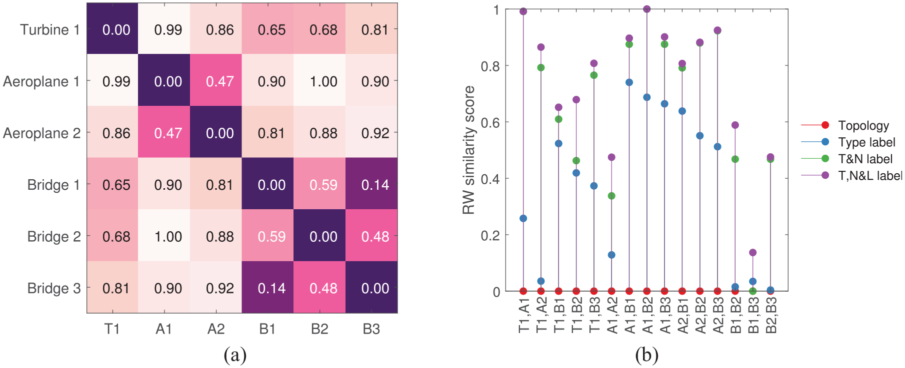
(a) The distance between graphs from section ‘The toy dataset’ calculated using the RW kernel. Here, the material properties, shape and volume of the nodes as well as the graph topology are included. (b) The kernel values when considering only topology (red) and when including the type kernel (blue), node-label kernel (green) and length kernel (purple).
Although the RW kernel was the first of its kind to incorporate continuous node attributes
42
and has shown to be useful in the context of PBSHM, it suffers from the problem of ‘tottering’; the RW kernel’s walks can revisit the same cycle of nodes leading to graphs with similar substructures to present artificially high similarities. Solutions to this problem have been found using the graph-invariant kernels
27
and the shortest path (SP) (a path is a walk without repeating nodes) kernel.
24
Although calculating all paths and longest paths is NP-hard, SPs can be computed in
The GraphHopper kernel
The GraphHopper (GH) kernel builds on the idea of comparing paths within graphs, where it counts simultaneous ‘hops’ along paths of discrete lengths. It is a sum of node kernels and is in the form,
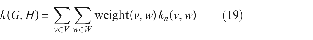
where
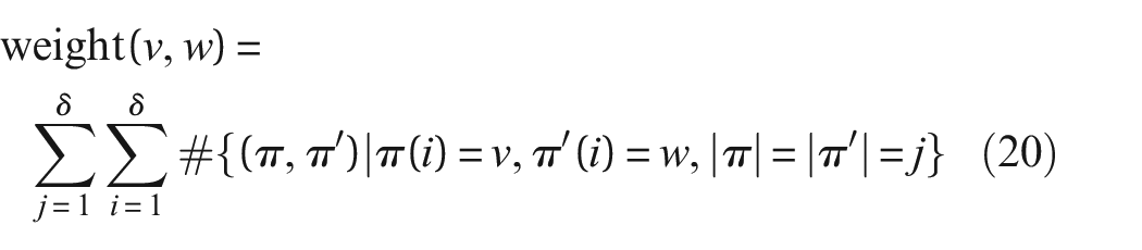
counts the number of times
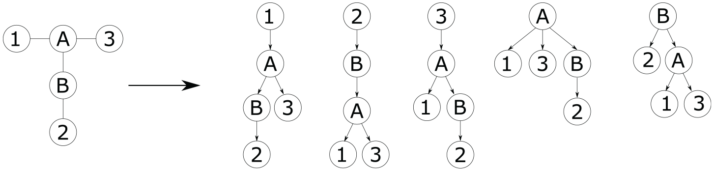
Graph of Bridge 1 on the right and the transition to the DAGs on the left.
The similarities measured across the population of toy structures in Figure 10(a) show that the GH kernel also groups the bridges together, and the aeroplanes together. However, the difference between the aeroplanes is much larger than that of the RW kernel, which makes physical sense as one plane is based on a large-scale passenger jet, whereas the other is based on a small, light propeller plane. When considering the bridges, the RW kernel results show different similarities compared to the GH kernel. For example, the RW kernel identifies Bridge 1 and 3 to be the most similar whereas the GH kernel detects Bridge 2 and 3 to be the most similar. The GH results in Figure 10(b) represent reality a little better here as it penalizes the differences in topology, material properties, type and sizes much more than the RW kernel, which only pulls Bridges 1 and 3 apart for difference in sizes (Figure 8(b)).
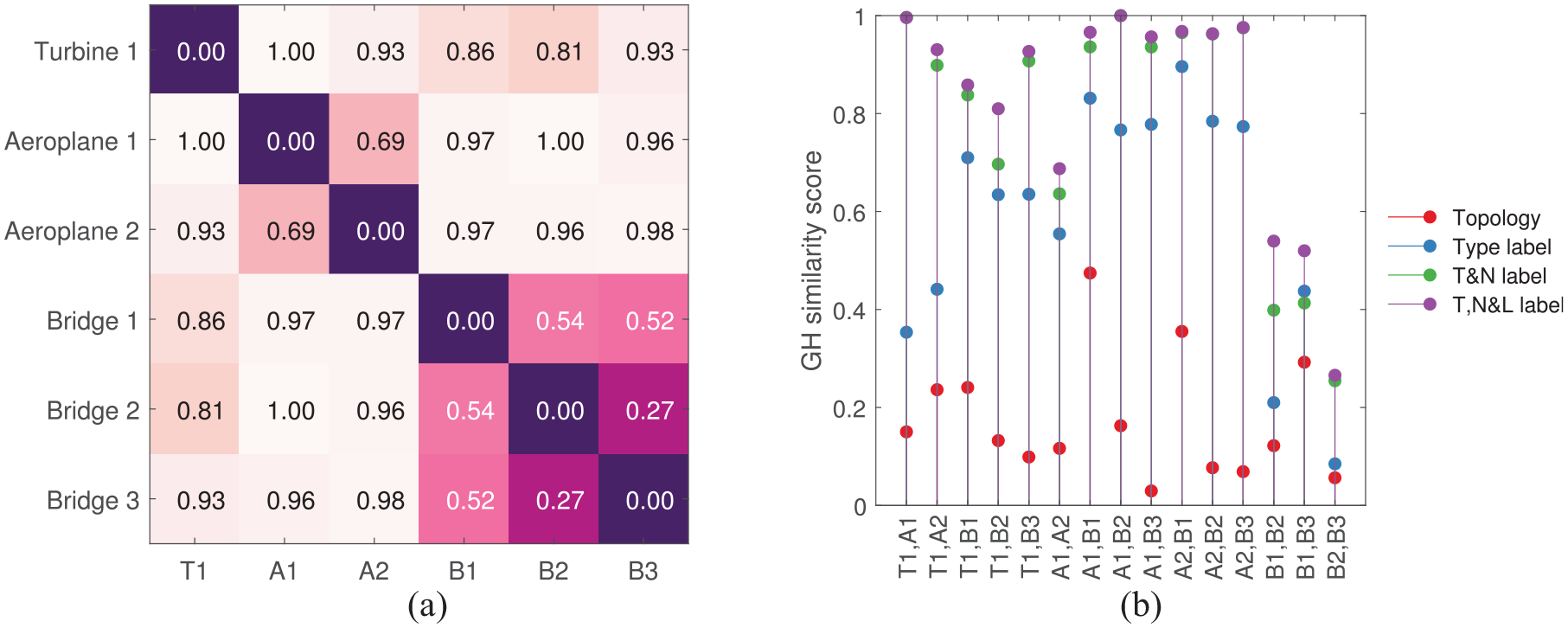
(a) The distance between graphs from section ‘The toy dataset’ calculated using the GraphHopper kernel. Here, the material properties, shape and volume of the nodes as well as the graph topology are included. (b) The kernel values when considering only topology (red), when including the type kernel (blue), including the type and node kernels (T&N in green), and including the type, node and length kernels (T,N&L in purple).
Figure 10(b) shows that the topological differences between the AGs are captured at a similar scale to attributes themselves, that is, the topological differences are in the range of
Compared to the RW kernel, the GH kernel has high dissimilarities between most structures because it does not suffer from tottering. Given the faster computation times and the resistance to tottering, the GH kernel is well suited for use in PBSHM for assessing structural similarity. In comparison to results from related work based on the Jaccard similarity and MCSs (that captures subgraph isomorphism) in Figure 4(a), the GH kernel has shown to be a good contender for structural similarity assessment in PBSHM; the GH kernel groups the bridges and the aeroplanes together, forming tighter communities than the Jaccard method where the distance between Bridge 1 and Bridge 3 are bigger than the distance between Turbine 1 and Bridge 2, for example. As a result, the GH results indicate that transfer is less risky between the bridges which makes practical sense.
Clearly, including attribute comparisons in the formulation has been an advantage in similarity comparison of structures, demonstrating the power of graph kernels in the context of PBSHM. In the next section, these graph kernels are used to assess the similarity of a heterogeneous population of real bridges, to evaluate their effectiveness and to gauge their usefulness for estimating the risk of negative transfer in PBSHM.
Case study: Measuring the similarity between a heterogeneous population of bridges
In the previous section, the use of graph kernels for assessing suitability of transfer learning in PBSHM was evaluated using a simulated toy dataset. The dataset was specially designed to draw out the differences between typical SHM structures to test the suitability of different similarity measures. In this case study, the aim is to test these measures on a dataset associated with real SHM structures in order to assess their performance for industrial application.
In this study, the similarity between a population of real bridges is measured, where the number of nodes (or individual components) in the bridges are much higher than the partition of structures into sub components within the toy dataset. One objective here, therefore, is to determine whether the graph kernels are able to handle larger datasets, to produce fast similarity comparisons. As the dataset only contains different types of bridges, another objective is to evaluate whether the graph kernels are sensitive to smaller changes within a population (in comparison to the toy datasets where the differences between the attributes and topology between the structures/AGs are much larger).
For the sake of simplicity, joints are not modelled in this case study; that is, there are no edge attributes.
The bridge dataset
The dataset used in this case study contains seven operational bridges from the United Kingdom. Specifically, it contains one arch bridge, one cable-stayed bridge, two beam-and-slab bridges, two truss bridges and a suspension bridge. The abstract graphical representations of the bridges with attributes highlighted are shown in Figure 11. The IEs of these bridges were specified in earlier work by Gosliga et al. 41 and reproduced here. An introduction to each graph is presented in this section. Table 4 provides a summary of the attributes included in each graph.
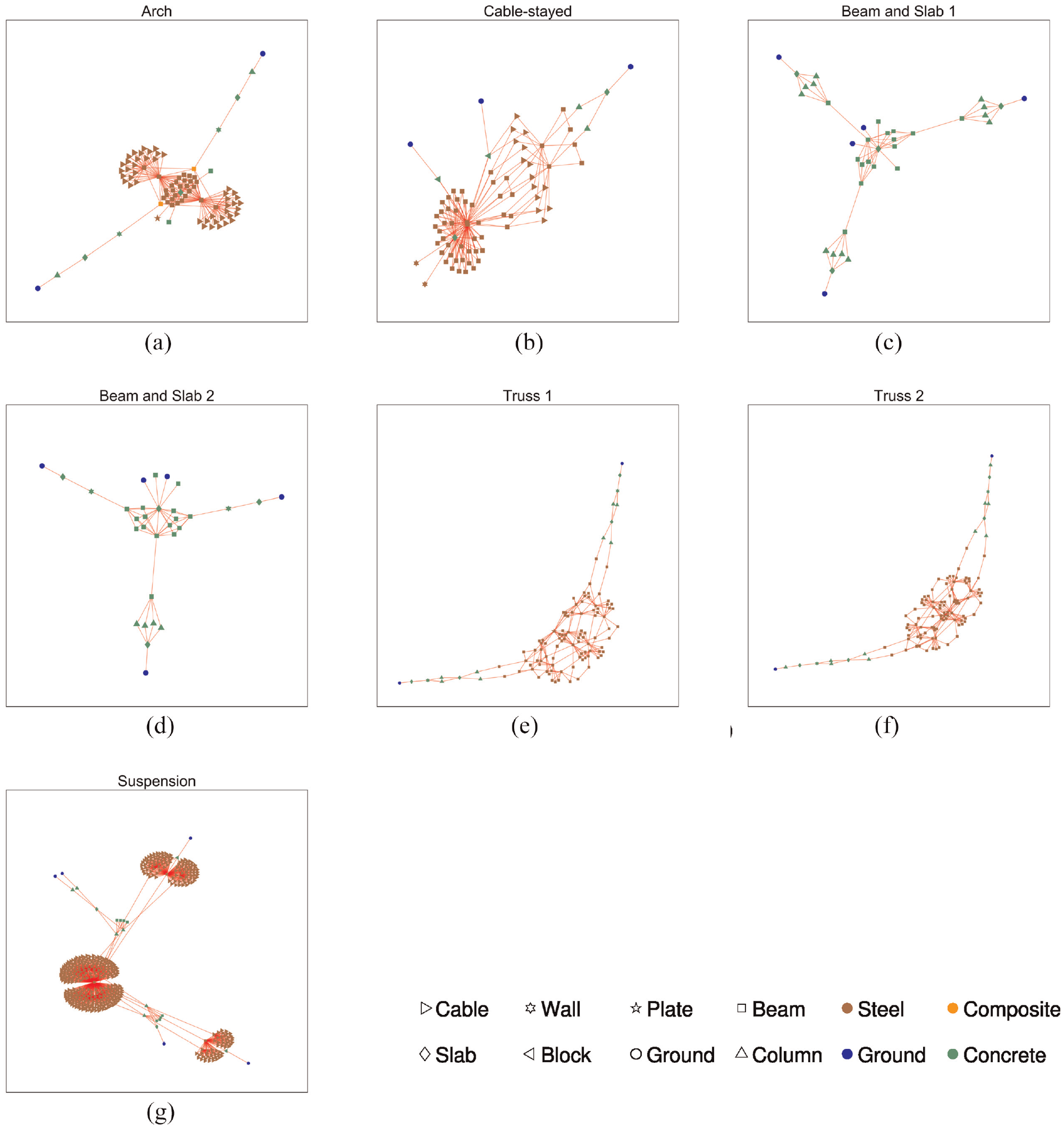
The graphs are: (a) The Arch bridge, (b) The Cable-stayed bridge, (c) The Bean and Slab Bridge 1, (d) The Beam and Slab bridge 2, (e), The Truss bridge 1, (f) The Truss bridge 2 and (g) The Suspension bridge.
Summary of the information contained in the AGs of the bridges in the dataset.
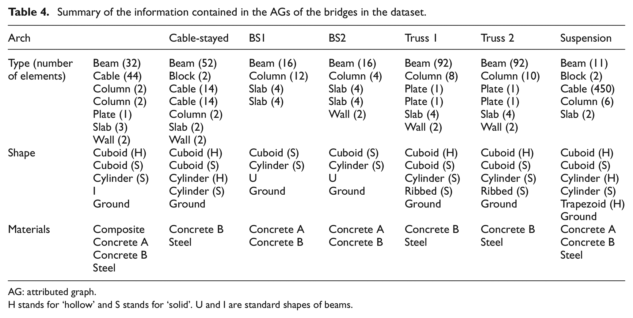
AG: attributed graph.
H stands for ‘hollow’ and S stands for ‘solid’. U and I are standard shapes of beams.
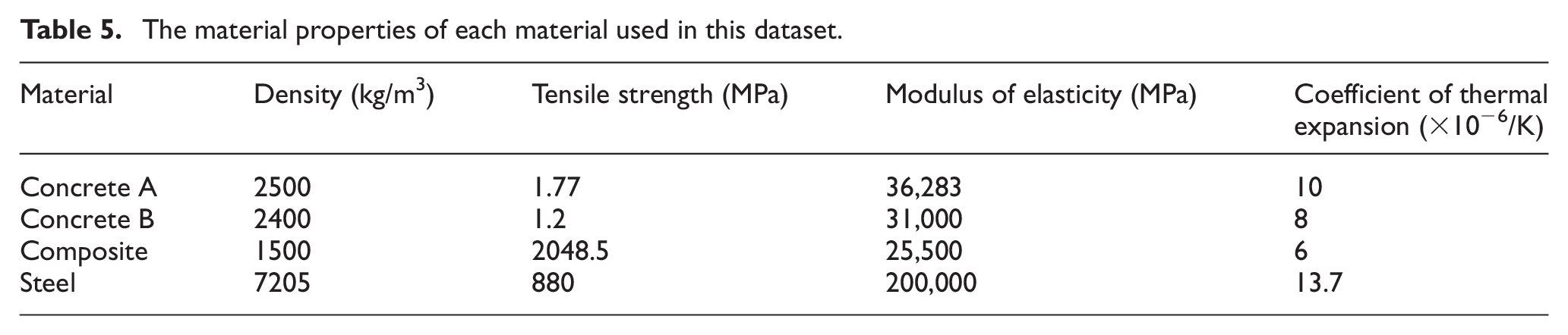
The element types encountered for the set of bridges include: beam, block, cable, column, plate, slab and wall. The shapes of the elements are cuboid (solid and hollow), cylinder (solid and hollow), ribbed (solid), trapezoid (hollow) and I and U (precast beam shapes). The materials consists of composites (GFRP), two types of concrete (A and B) and steel.30–34 The material properties included are density (kg/m3), tensile strength (MPa), modulus of elasticity (MPa) and coefficient of thermal expansion
The material properties of each material used in this dataset.
Arch bridge
Located in Northern Ireland, the tied-arch bridge in this case study (referred to as the ‘Arch’ bridge or AR, henceforth) has a span of 103 m and is composed of steel. The deck in these types of bridges is supported by arches that span between supports. The arch can be supported on struts where the deck is above the arch or the arch is supported by hangers where the deck is below the arch. The arch bridge in this dataset contains two arches at either side of the deck which is supported by longitudinal girders and transverse beams. Figure 12 presents a photo and a drawing of the bridge and Figure 11(a) shows the corresponding graph with attributes. Table 4 details the summary of element types, shapes and material properties of the Arch bridge.
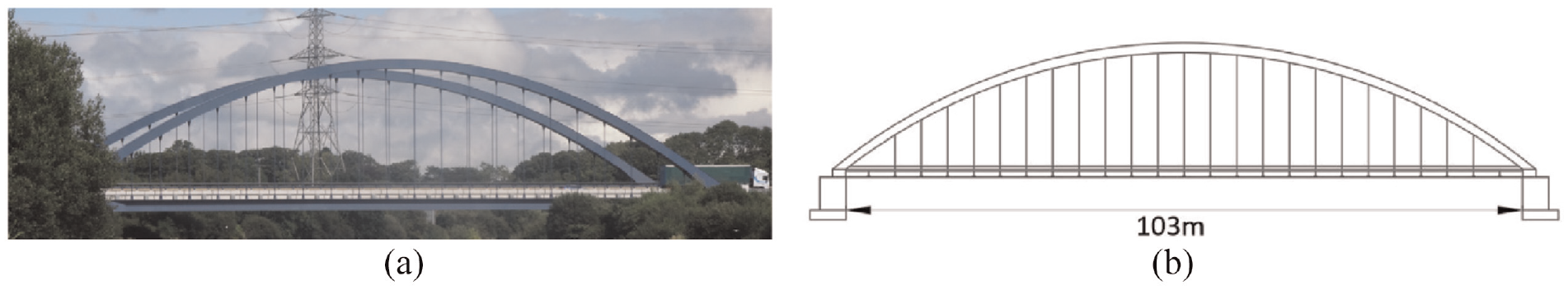
(a) A photograph of the tied arch bridge. (b) A schematic of the bridge.
Cable-stayed bridge
The bridge dataset contains one cable-stayed footbridge referred to as ‘Cable-Stayed’ or CS here. In this particular bridge, that is located in Exeter, the deck is supported by transverse beams and longitudinal girders and cables that are themselves connected to pylons. A photo and a drawing of the bridge is presented in Figure 13. The graphical representation and the AG of the bridge (with material properties and element types) can be found in Figure 11(b). Table 4 presents the attributes in the AG of the cable-stayed bridge.
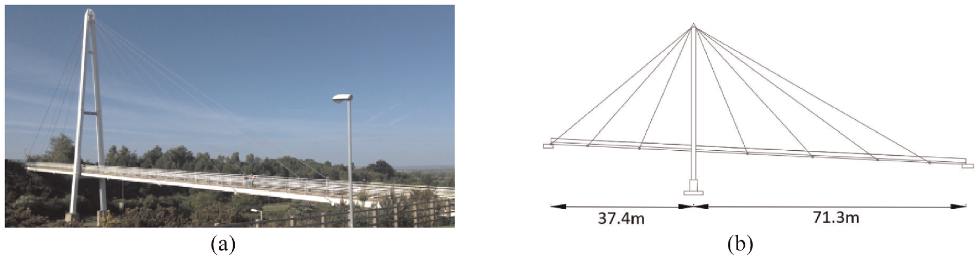
(a) A photograph of the cable-stayed bridge. (b) A schematic of the bridge.
Beam-and-slab bridges
The dataset contains two real integral-abutment beam-and-slab bridges located in Northern Ireland, named here as ‘Beam and Slab 1’ (BS1) and ‘Beam and Slab 2’ (BS2). Both bridges are made of reinforced concrete and have a similar topology. Essentially, these bridges contain beams that run along the span of the bridge with cylindrical columns to support the decks. Figure 11(c) and (d) present the graph of the beam-and-slab bridges that includes the type and material property information. Table 4 summarizes the types of elements in the AGs as well as their shapes and material properties. Figures 14 and 15 present images of the bridges.
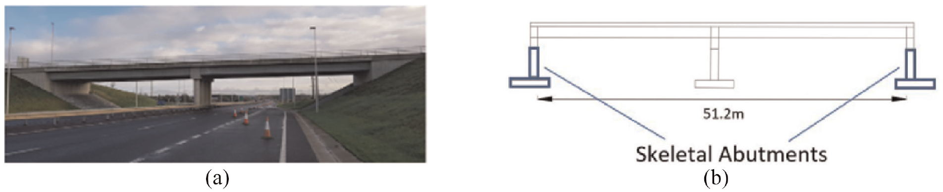
(a) A photograph of Beam and Slab 1. (b) A schematic of the bridge.
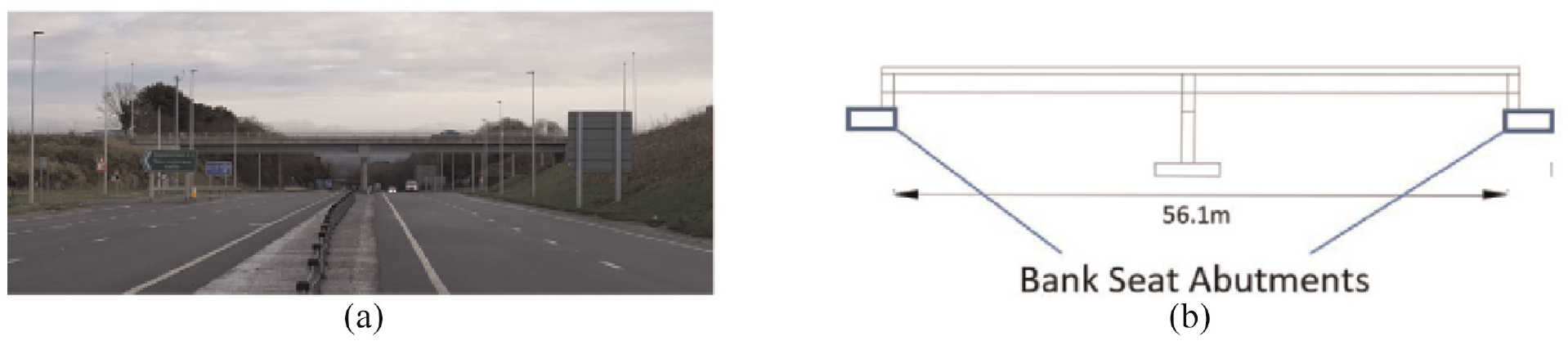
(a) A photograph of Beam and Slab 2 (b) A schematic of the bridge.
The main differences between the bridges stem from the type of abutments and number of beams per span:
BS1 contains skeletal abutments designed to flex with deck movement, and BS2 contains bank-seat abutments.
BS1 comprise of four precast longitudinal beams per span, and BS2 has a slightly longer span and contains five beams.
In BS1, the abutment and intermediate pier each comprise a foundation slab and four columns with a cap beam on top. In BS2, only the intermediate pier is supported by four cylindrical columns as a result of the bank-seat abutments.
Truss bridges
Located in Northern Ireland, Truss 1 (TR1) is footbridge with a span of 36 m that contains a Warren type truss for both walls. It is a simply supported single-span bridge with pad foundations. The deck of this particular bridge is placed below the truss. Truss 1 bridge also contains transverse beam elements and continuous bottom chords that support the deck. Figure 16 shows a photograph and a drawing of Truss 1 footbridge. Figure 11(e) presents the abstract graphical representation of the Truss 1 bridge and its included attributes. The description of the elements in Truss 1 bridge can be found in Table 4. The second truss bridge, referred to in this paper as ‘Truss 2’ (Figure 11(f)) only differs very slightly from Truss 1. Truss 2 (TR2) has a shorter span (by 2 m) and contains piled foundations. A photograph and a drawing of Truss 2 is presented in Figure 17.
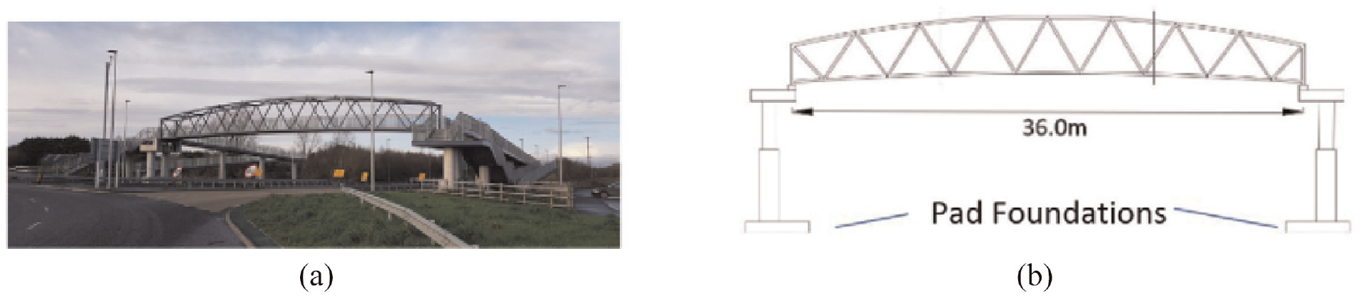
(a) A photograph of Truss 1. (b) A schematic of the bridge.
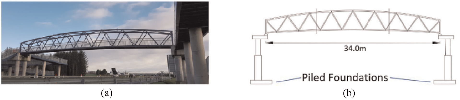
(a) A photograph of Truss 2. (b) A schematic of the bridge.
The suspension bridge
The suspension bridge considered here is the Humber bridge, an iconic bridge in the north of England joining the city of Kingston-upon-Hull to the town of Barton-on-Humber and crossing the river Humber. A photograph of the bridge is given in Figure 18, while the abstract representation is given in Figure 11(g). It is a single-span road bridge of length 2.2 km; at the time of its construction it was the longest bridge of its kind in the world. A detailed description would constitute a major digression; however, various references can be found in The Humber Bridge Board. 54
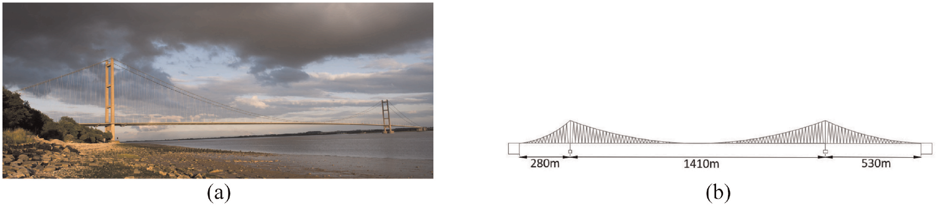
(a) A photograph of the Suspension bridge. (b) A schematic of the bridge.
Results and discussions
To measure the structural similarity of the heterogeneous population of aforementioned bridges, the RW and GH methods suggested in section ‘Graph kernels’ are employed, because they have the ability to include discrete and continuous attributes. For the length kernel, a value of 1000 is set for
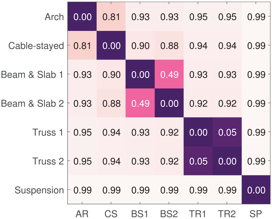
The confusion matrices in Figure 19(a) and (b) represent the RW and GH kernel values (respectively) between each of the seven bridges, when including the geometry classes, material properties and the element sizes.
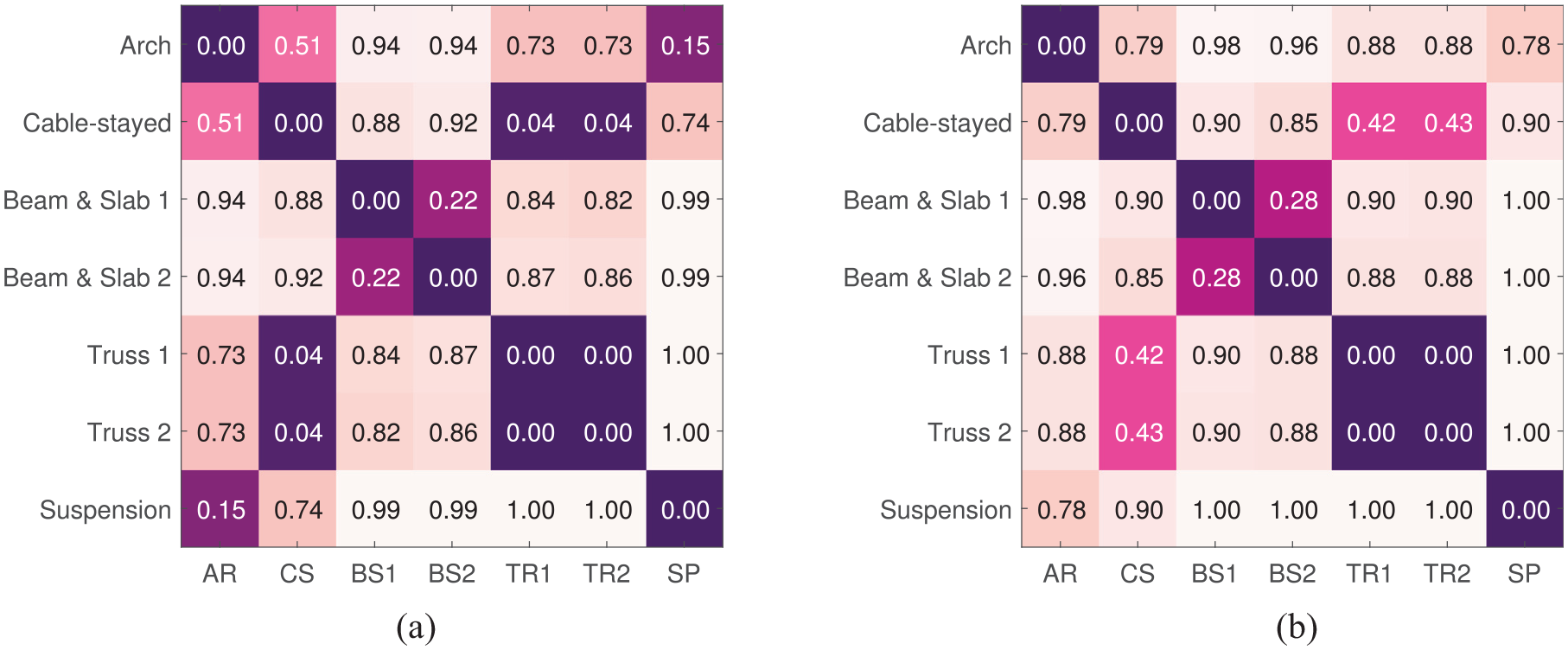
The similarity between the bridges calculated using the (a) RW kernel and (b) GH kernel when taking into account the topology, type, node-label and length kernels.
At first glance, it is clear that the results of the graph kernel comparisons in Figure 19(a) and (b) are sensible and follow engineering knowledge; the bridges that have a similar construction are grouped together. This is a major finding, as the ability to compare continuous node attributes within the similarity formulation allows for many possibilities in the future. For example, it may be possible to include time-series data from a sensor located at a specific element of an AG. Furthermore, the computational complexities of the graph-kernel methods proposed here are sensible. The GH kernel can be computed in
Some of the interesting observations from Figure 19(a), (b), Figure 20(a) and (b) are:
The two truss bridges are found to be almost identical in structural similarity with values of
The two beam-and-slab bridges are also found to be similar within the population, but with a higher value of 0.22 (RW kernel) and 0.28 (GH kernel) compared to the truss bridges. The middle section of the beam and slab bridges share a similar construction, although the end sections do not, 41 leading to the larger distances between them in comparison to the distances between the truss bridges.
It is possible that the RW kernel is suffering from ‘tottering’ here; the similarity between the cable-stayed bridge versus the truss bridges are much lower compared to the similarity values between the two beam and slab bridges, suggesting a high artificial similarity in the former case. As the scale of similarity is arbitrary, that is, the values of similarity are dependent on the type of graph kernels used, the useful information here is the similarity values across the population. To that end, the results from the GH kernel in this scenario are less surprising and make physical sense, because they find the difference between the cable-stayed bridge and the truss bridges to be larger than the difference between the beam-and-slab bridges. The GH kernel is better suited here, as it avoids the problem of tottering.
It is worth dwelling somewhat on the comparisons with the suspension bridge (last row of confusion matrices). As one might expect, there are significant differences with the beam-and-slab bridges; the rest of the entries are interesting. In simple terms, the other bridges share a certain geometrical nature, in that there are superstructures on either side of the deck joined by hangers to deck level. The closest match is between the arch bridge and the suspension bridge (metric value of 0.15 (RW) and 0.78 (GH)); this arguably makes sense because the topological characteristics of the hangers match. In these two bridges, the hangers are vertical, so they each meet both the superstructure and deck with single graph edges. The next closest match is with the cable-stayed bridge (metric of 0.74 (RW) and 0.9 (GH)); one might argue that this distance is greater because the deck connections are simple edges once more, but the connection to the superstructure has multiple cables connected at the tower. Finally, the truss bridges appear very different from the suspension bridge; again this seems to make sense from a topology point of view, as at the points at which the ‘hangers’ meet the superstructure or deck, they also meet other ‘hangers’. The bridges are distinguished by the topology of the connections in their superstructure. Of course, there are also matters of scale to consider.
AG similarity and transfer learning
Both confusion matrices in Figure 19(a) and (b) present high similarity scores between the cable-stayed bridge and the truss bridges. The high similarity between these bridges stems from the similarity in compared attributes, as seen in Figure 22; the truss bridges and the cable-stayed bridge are both made up of the same materials and have similar components of similar sizes. These results suggest that the risk of negative transfer is lower between the truss bridges and the cable-stayed bridge compared to the others in the population. To evaluate this outcome, consider an example where a target structure within transfer learning is a truss bridge with a damaged truss. These results suggest that a loss of tension in a cable within the cable-stayed bridge may be comparable to the presence of damage in a truss within the truss bridges. As a result, the cable-stayed bridge may be used as the source structure here, provided that it contains labelled information. It makes sense not to use the beam-and-slab bridges for transfer here as they do not contain any metal components or overhead support structures such as cables or trusses (as reflected in the low similarity scores). Although visually, the arch bridge may also be a likely candidate for transfer (as the arch bridge contains metal overhead support archers connected to a deck, similar to a truss bridge), greater topological differences as well as disparities in the type, materials, and the size of the components make the arch bridge an unsuitable candidate.
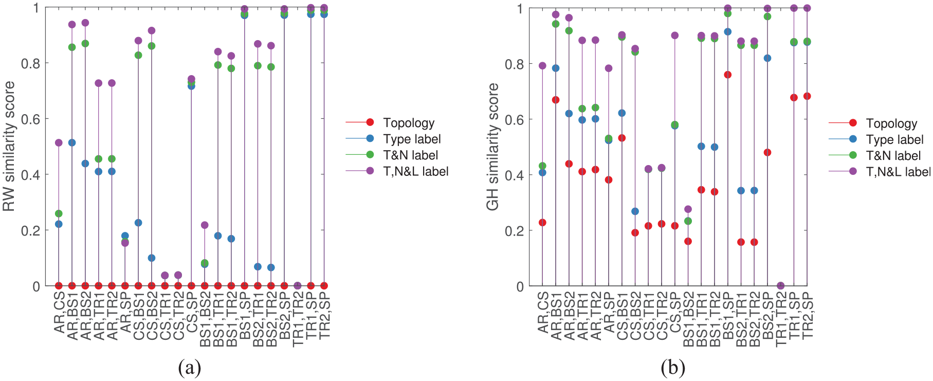
The kernel values of (a) the RW kernel and (b) the GH kernel when considering only topology (red), when including the type kernel (blue), including the type and node kernels (T&N in green), and including the type, node and length kernels (T,N&L in purple).
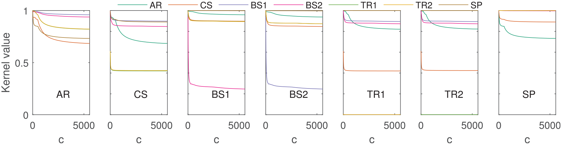
The behaviour of the length kernel as the value of constant
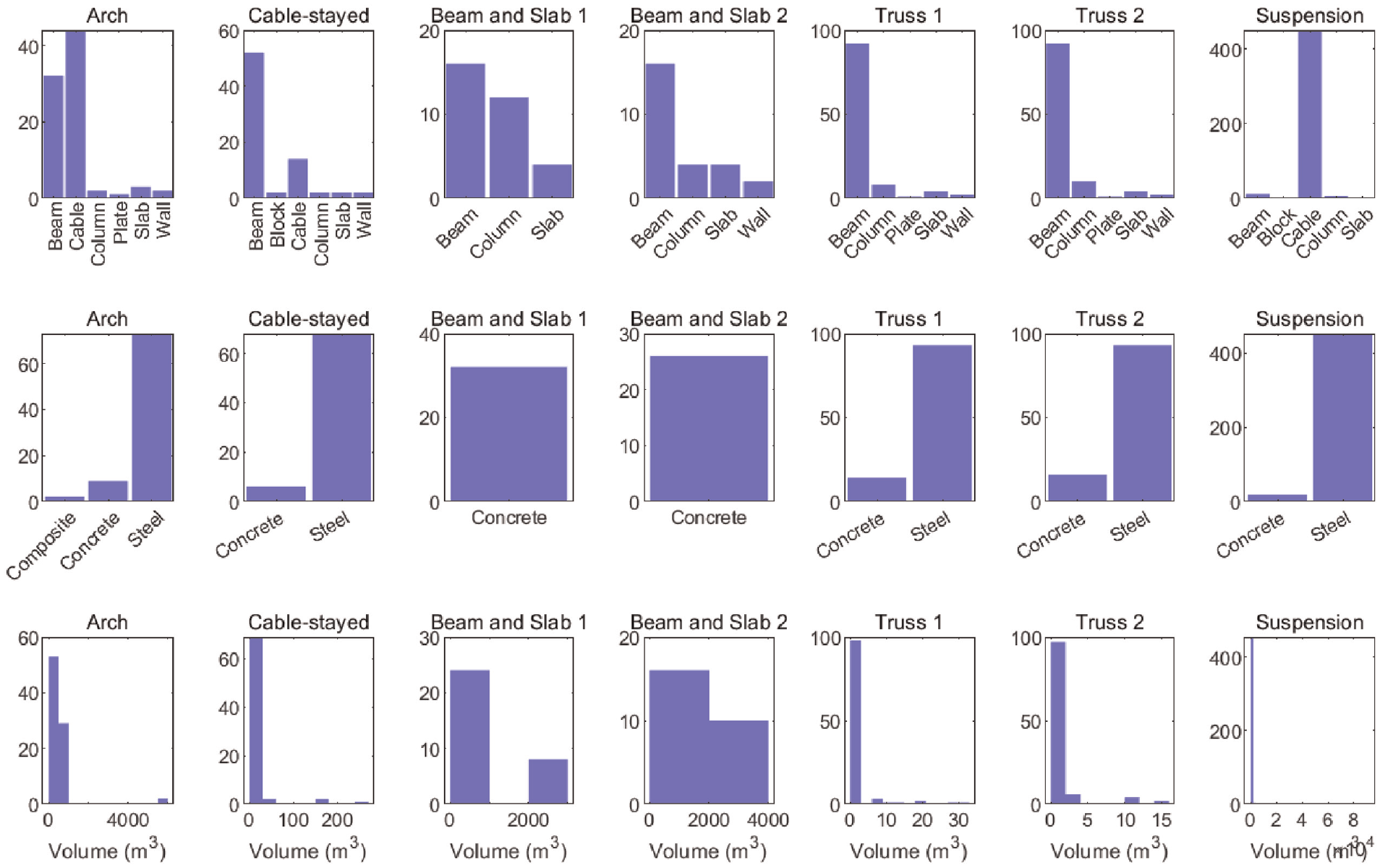
The attributes of the bridge dataset where the y-axis represents the number of nodes containing the specific attribute. It is clear that the cable-stayed bridge has similar attributes to the two Truss bridges, giving a high similarity scores within the graph kernel formulations.
There are clearly many benefits to using the proposed graph kernel approach set out in this paper to help evaluate the risk of negative transfer in PBSHM. Consequently, it may be useful to consider threshold values to determine a point at which the similarity values should be discounted for transfer learning, in order to avoid negative transfer across a population. Taking the earlier example of transfer between the cable-stayed bridge and the truss bridge, consider setting a threshold at a similarity value of 0.5. The idea here is that if the kernel value between these two bridges surpass 0.5, then transfer should not be conducted. Figure 23(a) presents this scenario using the GH kernel results of Truss bridge 1 versus the cable-stayed bridge and the arch bridge. It is clear that the arch bridge crosses this threshold, suggesting a high risk of negative transfer. Figure 23(b) presents a similar scenario where a threshold is used to evaluate which bridges are suitable to transfer information when beam-and-slab 1 is the target structure. Here, all bridges besides beam-and-slab 2 cross the threshold, making them unviable for transfer, where the arch bridge is the most likely candidate source structure that will result in negative transfer. These results closely follow the assumptions made in the original framework of structural similarity assessments set forth by Worden et al. 22 in the paper ‘When is a bridge not an aeroplane?’, thus verifying those findings with a suitable metric.
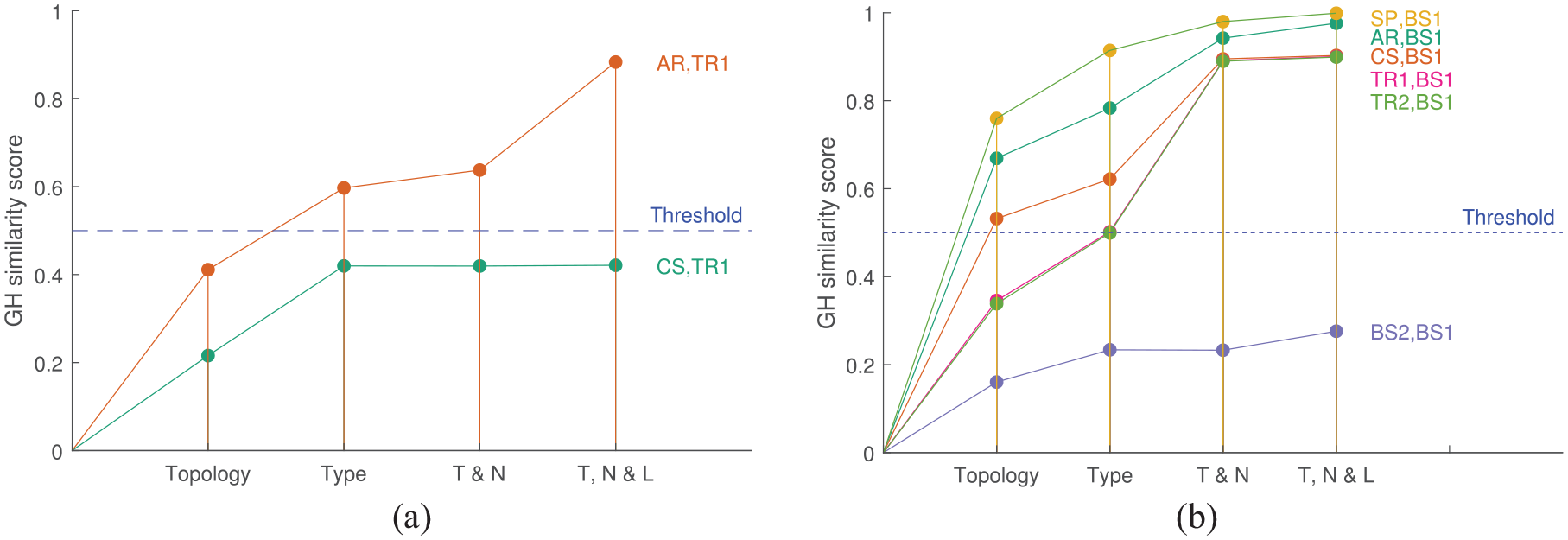
Setting a manual threshold for transfer learning to find suitable source structures for a given target structure. (a) When the target structure is TR1, source structures AR is unsuitable as it has crossed the threshold. Source structure CS may be suitable for transfer. (b) When the target structure BS1, BS2 is a suitable source structure (considering all others) given the threshold. Here, the similarity values provided when considering only topology, when including the type kernel, including the type and node-label kernels (T&N), and including the type, node-label and length kernels (T,N&L). (a) Identifying source structures for TR1. (b) Identifying source structures for BS1.
This section has demonstrated that graph kernels can be used as similarity measure with desirable properties that serve as a metric in the space of AGs/base space. The available kernels not only capture the substructure isomorphisms within the population well, they are also able to assess the attributes within the graphs, providing a complete picture of the differences. Next, a comparison between the proposed graph kernels method and the current MCS-based methods is undertaken to highlight the advantages of the graph kernels methodology.
The proposed graph kernels versus the current methods used in PBSHM
For comparison against the proposed graph kernels methods in this paper, the current methods of similarity assessment of structures in PBSHM that utilizes the Jaccard distance and MCSs is reproduced from Gosliga et al. 41 in Figure 24.
The Jaccard distance when considering the size of the common maximum subgraph between structures with attribute matching. This figure is reproduced from the work by Gosliga et al. 41
Figure 24 presents the similarity of the bridge dataset when using the MCSs – which provide information related to the sub-structures – of the bridges along with discrete node comparisons (similar to applying the type kernel in the graph kernels method). The approach has led to sensible results that follow engineering judgement. 41 However, there are two major drawbacks to consider. Firstly, the Jaccard + MCS method is unable to assess continuous node attributes. Secondly, the computational efficiency of obtaining an MCS is NP-complete, leading to significant computational times (in the 102 h range) when considering the large AGs of these bridges. Graph kernels are a helpful solution here as they can incorporate continuous node attributes and give a measure of scale of the nodes, while computing the similarities within seconds. Table 6 summarizes the current state-of-the-art method of assessing structural similarity in PBSHM (Jaccard distance calculated on MCSs) and the graph kernels method proposed in this paper.
Summary of methods applied in PBSHM for assessing similarity of graphs.
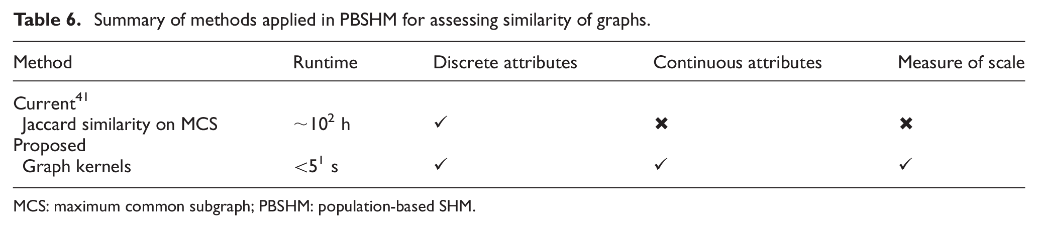
MCS: maximum common subgraph; PBSHM: population-based SHM.
Conclusions and future work
PBSHM was proposed as a solution to address the drawbacks of SHM related to lack of labelled data. The idea is to share labelled information between similarly-behaving structures via transfer learning, in order to increase the pool of available information and improve the performances of learners across a range of SHM behaviours. To assess similarities within populations to find suitable candidates for transfer, metrics are required to measure similarities in the collected data and the structures themselves; the assumption is that ‘similarity in data suggests similarity in structures’ and ‘similarity in structures’ suggests ‘similarity in data’. In this paper, the focus was to find metrics that can assess the similarity of structures.
By treating structures as AGs, this is the first study to use graph kernels to assess various aspects of SHM structures including their topology, geometry, scale and material properties. Graph kernels show similar behaviours to distance metrics, and serve as suitable metrics within the space of graphs/structures. The inclusion of node attributes pulled dissimilar structures apart within the space of graphs, verifying the findings/assumptions from earlier studies on this topic. 22 The suitability of graph kernels was first demonstrated on a population of simulated toy structures where they were able to group similar structures such as bridges together. Later, the metrics were tested on a group of real, operational bridges, where they identified structures of similar construction to be suitable for transfer. The results suggested that the GH kernel based on measuring SPs is well suited for assessing similarity for PBSHM as it can handle discrete and continuous node attributes, has runtimes in the range of 5 1 s, and does not suffer from ‘tottering’. In this paper, manual thresholds were set in order to separate appropriate structures for transfer. In future work, principled methods of determining automatic thresholds will be studied.
Compared to previous methods based on the Jaccard index and MCSs, the graph kernel methods were better suited for industrial application of PBSHM; the graph kernels assessed the substructure isormorphisms between graphs in a fraction of the time, where some graph kernels (the RW kernel and GH kernel) were able to assess both continuous and discrete node labels. As previous methods are unable to assess continuous node attributes, the graph kernels provide a considerable advantage for PBSHM. The hope is that, in future work, sensor data can be included in the formulation as continuous attributes, allowing this framework to simultaneously assess structure and feature data.
In this paper, joint information was not included for simplicity and because methods of defining joints for PBSHM are currently ongoing. As a result, methods of modelling joints will be conducted in future work.
Footnotes
Declaration of conflicting interests
The author(s) declared no potential conflicts of interest with respect to the research, authorship, and/or publication of this article.
Funding
The author(s) disclosed receipt of the following financial support for the research, authorship, and/or publication of this article: This work has been supported by the UK Engineering and Physical Sciences Research Council (EPSRC), via the project A New Partnership in Offshore Wind (grant numbers EP/K003836/2 and EP/R004900/1). K.W. also gratefully acknowledges support from the EPSRC via grant number EP/J016942/1 and E.J.C. is grateful to EPSRC for support via grant number EP/S001565/1. The authors would also like to thank Queens University Belfast for providing the bridge dataset used for this work. For the purpose of open access, the author has applied a Creative Commons Attribution (CC BY) licence to any Author Accepted Manuscript version arising.