
Abstract
Damage detection is perhaps the most critical objective of structural health monitoring. Proper documentation of the progression of structural damage from onset to failure enables performance-based maintenance that mitigates risk and contains socioeconomic impact. Recently, damage detection methods that focus on change detection through analyses of the structural global response in the frequency or time domain have garnered attention due to their efficiency and accuracy. This work proposes a novel time-domain, nonparametric, data-driven change detection method. The time-domain B-Spline transfer function is defined as a signature time history response of the structure, referred to in this work as the B-Spline signature response (BSR). BSR may be computed directly through a physics-based simulation, or it be extracted in a discrete form from measurements of displacement, velocity, or acceleration time histories of structural response to any external excitation. The BSR is independent of loading, is a characteristic of the system, and captures the condition of the structure at the time of acquisition without the need for identifying structural properties. In this work, the fundamentals of the BSR concept are introduced first along with the process of extracting a BSR from structural responses to arbitrary excitations. Verification and validation studies are conducted based on computer simulations and laboratory testing and are discussed in detail. Subsequently, an approach is proposed to detect change through correlation of BSR signals acquired at different times during the monitoring period. Any changes in the intrinsic characteristics affecting the response cause BSR changes and correlation loss. The change detection methodology is demonstrated through computer simulations and experimental investigations. Initial parametric studies are conducted to investigate the suitability of the proposed approach to detect small structural changes. This article demonstrates the validity of the proposed method and establishes the framework for further development and case-specific applications.
Keywords
Introduction
Maintaining civil infrastructure in a state of good repair is critical to the quality and safety of daily life, yet deterioration over time is inevitable. As structures age, the state of the structure changes, and damage accumulates due to both environmental and mechanical factors, which ultimately leads to some type of failure. It is key to document this progression to failure to accurately predict the structure’s service life and prevent catastrophic and tragic accidents, such as the 2021 Surfside building collapse in Miami, Florida, or the 2018 Morandi Bridge collapse in Genoa, Italy.1,2 A less visible but equally important factor in damage mitigation and failure prevention is the need to prioritize and optimize maintenance strategies to reduce the massive associated maintenance costs. This is evident in the nearly 1 trillion USD invested into civil infrastructure by the United States in 2021 or the more than 500 billion USD similarly invested by China in 2013.3,4Exempli gratia, as of 2022 more than half of the more than 600,000 highway bridges in the United States are in fair or poor condition and in need of repairs or replacement, 5 and new bridges are being built larger than ever before with higher vehicle loading as demand increases.6–8 Even localized damages or elevated stress fields can increase the rate of structural deterioration and affect the general response of a structure.9–12 These impediments underscore the need to better understand the changes of the state and performance of the built environment over time.
The issues regarding structural deterioration have prompted research since the early 1970s, which has led to the emergence of structural damage detection (SDD) technologies. SDD is a subset of structural health monitoring (SHM), which is the process of implementing a damage detection strategy and documenting the progression of damage from onset to failure. Abdo 13 provides a foundational review of the SHM field for further reading. Within SHM, SDD is typically accompanied by pre- or postprocessing of data which can be computationally expensive. 14 SDD technologies targeted at specific locations are known as local techniques, as opposed to global techniques wherein the global response of the structure is analyzed. Global methods have several benefits over local testing, namely no requirement for a network of closely spaced sensors, no requirement for knowing the approximate area suspected of damage, and instrumentation can be easily carried, handled, and attached to structures. 14 These advantages significantly reduce the time needed to inspect a structure when compared to local methods. However, damage is typically a local phenomenon that may not significantly alter the global response of structures. This presents a challenge in how to optimize the detection and correlation of small changes in global response to local damage, particularly in a noisy environment.
Global methods can be broadly categorized into physics-based or data-driven methods. Physics-based methods involve iteratively updating the parameters in a detailed computer simulation model of the structure until the response of the simulated structure to a known excitation matches the response obtained by a network of sensors on the real-world structure.15,16 The updated parameters can then be corresponded to damage. In contrast, data-driven methods determine structural characteristics by analysis of response data from the structure, with recent research focusing on detecting structural change rather than structural damage, where the structural change is indicative of structural damage. Data-driven methods have distinct advantages: no requirement of a detailed computer simulation model nor an extensive network of sensors. However, these methods need to address the ill-posedness of inverse problems and model errors, for which data regularization is commonly used Guo et al. 17 and Yang. 18
Parametric data-driven methods typically aim to determine modal parameters such as natural frequencies, modal flexibility, modal damping, or strain energy from measured responses.19–21 Deviation from a baseline is used to recognize damage. Recently, research has implemented autoregressive analyses to quantify the link between mechanical properties of a system and the regression model parameters.22,23 One critical component of parametric methods is the high sensitivity to noise, particularly fluctuating ambient conditions, which can significantly influence the estimated parameter values. Attempts to reduce this kind of uncertainty have produced new regression models and is the focus of much research effort. 24
On the other hand, nonparametric data-driven methods exploit signal processing techniques to identify damage directly from measured signals, often with the aid of machine learning algorithms.14,25,26 One key advantage of nonparametric methods is that there is inherent accounting for uncertainties in measurements and environmental factors through statistical tools. 27 The analysis can occur in the frequency domain, using wavelets or Hilbert–Huang transform, for example.28–30 These methods are capable of detecting damage from nonlinear and nonstationary data and can be combined with other intelligence algorithms like neural networks to develop quick processing tools. 31 Frequency response functions (FRFs) can be used to determine damage via the difference between the vibrational amplitude actually measured and the vibrational amplitude computed at the same location via interpolation of values measured at other locations.32,33 Systems are also often analyzed in the time domain where changes in the time history response due to an external load can identify damage without needing the additional steps for frequency domain transformation.27,34 Time history analyses utilizing B-Splines as time-domain transfer functions have been implemented for 3-D elastodynamic analyses, 35 dynamic and seismic analyses of foundations, 36 transient response analyses of sleepers in railway lines, 37 transient soil-structure interaction analyses of rigid foundations, 38 and fluid-structure interaction analyses of rigid bodies. 39
This work introduces the fundamentals of a data-driven approach for change detection within the framework of the B-Spline signature response (BSR) techniques. The BSR captures in a single, discrete time-domain, response function the combined effects of the intrinsic system attributes at a particular point in time during the life of the structure that affects its dynamic response to any excitation, without explicitly quantifying the individual attributes a priori. Such attributes include the spatial configuration, material properties, boundary conditions, and any existing damage or deterioration at the time of the BSR extraction. The BSR is independent of external excitations, and it forms a basis function of the system response to any external excitation. A single BSR, by itself, does not detect structural changes. Rather, structural changes are identified as deviations of any BSR from its baseline. Because BSR captures the combined effects of all system attributes in a single function, the fundamental form of the BSR-based change detection presented in this work does not identify the source of the structural change. The implementation and feasibility of the proposed concept is demonstrated through numerical studies and laboratory experiments. The nature of the BSR reduces the instrumentation demands and computational resources. The work presented in this article sets the foundations for the development of a new generation of BSR-based SHM techniques or the potential for improvement of existing technologies.
Mathematical background
The B-Spline polynomial
B-Spline polynomials belong to a family of basis functions used in data interpolation and approximation. The B-Spline functions are piecewise smooth polynomials of order k derived based on a knot sequence
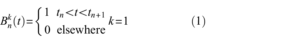
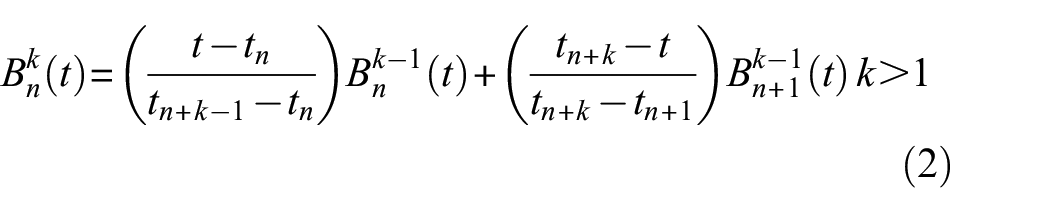
The
where
Since the
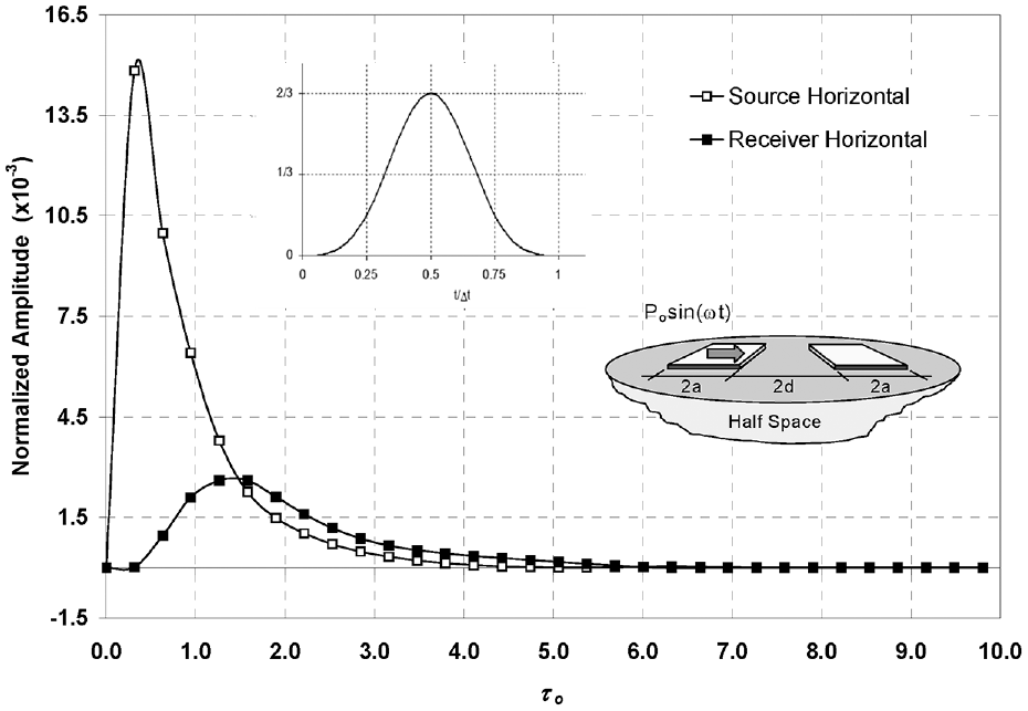
Example of discrete BSR functions of rigid surface foundations.
The B-Spline signature response
A time-domain B-Spline transfer function is a continuous function in time that is defined between any two points
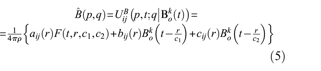
where ρ, c1, and c2 are, respectively, the mass density, pressure wave, and shear wave velocities of the medium and i, j = 1,2,3 are the principal directions of the cartesian coordinate system. In this case, the BSR function, Uij, represents the time history of the displacement response in the “i”direction at the receiver point p caused by a B-Spline,
The dynamic system in this example consists of two rigid square foundations of side 2a resting on an elastic half space, as shown in the inset of the figure. The edge-to-edge distance between the footings is 2d. Since the footings are considered rigid, the motion of the foundation system is fully defined by 12 DOF, that is, three translational and three rotational DOF at each footing center. The direct time domain BEM reported in Stehmeyer and Rizos,
38
is used to compute the response of both foundations when a fourth-order B-Spline force is applied at the source footing on the left, as shown in the inset of the figure. The two BSR curves shown in Figure 1 represent the normalized amplitude of the horizontal translation of the centers of each footing as a function of a nondimensional time parameter,
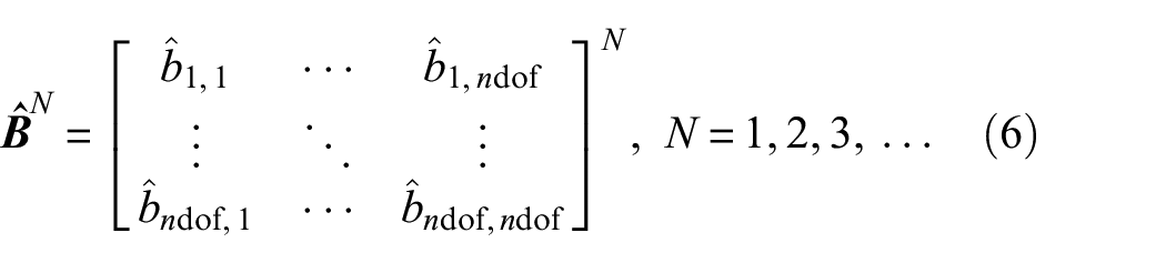
In Equation (6), matrix
a. The BSR is independent of any external excitations. In fact, during loading of time invariant dynamic systems, the BSR is invariant and, therefore, is considered a signature response that captures the current state of the dynamical system. Further, the BSR is dependent only on intrinsic characteristics affecting the dynamic response, including the spatial configuration, material properties, boundary conditions, and any existing damage or deterioration at the time of the BSR extraction. Any changes of these structural characteristics alter the BSR, which is the basis for the change detection method proposed in section “BSR change detection method.”
b. The BSR invariance implies linearity; however, this concept may be extended to include material or geometric nonlinear structures at “the secant state”. In such cases, the BSR invariance would hold with the condition of small perturbations from the baseline state. In a reciprocal approach, the BSR invariance in linear systems may be of value in detecting nonlinear structural response due to material or geometric nonlinearities, which are often attributed to structural damage.
c. In order to obtain the most general form of
d. While the BSR is computed efficiently in numerical models of the physical systems in a direct manner, it is almost impossible to measure the BSR directly in physical systems due to the difficulty of accurately reproducing the B-Spline loading with mechanical means. However, the computational efficiency of extracting BSRs from any response time history, as discussed in section “The inverse problem,” mitigates the issue and shows promise for real-time applications.
e. The BSR is obtained through analyzing the measured time history response and inherently contains uncertainties in the measurements and environmental factors. Thus, a statistical approach will be required with implementation. The first step is to establish the framework for extracting BSRs in a deterministic manner before addressing noise in measurements due to variation in operational or environmental conditions. This work details the methodology of extracting BSRs and identifying damage in a deterministic manner, which will become the basis for statistical analysis in future work.
Using BSRs to predict dynamic response to arbitrary excitation
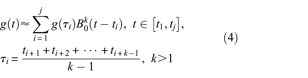
The function interpolation scheme using B-Spline polynomials shown in Equation (4) indicates that if the BSRs of a system are known, then the response to an arbitrary excitation can be computed as a mere superposition of the BSRs without further consideration of the system itself, as demonstrated in Figure 2.
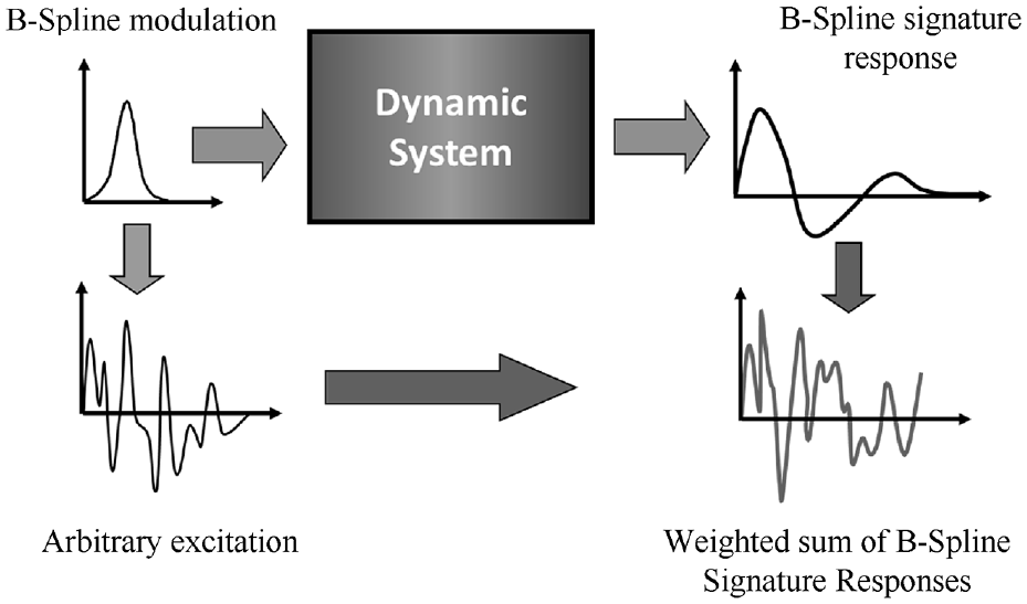
Response to arbitrary excitation using BSR functions.
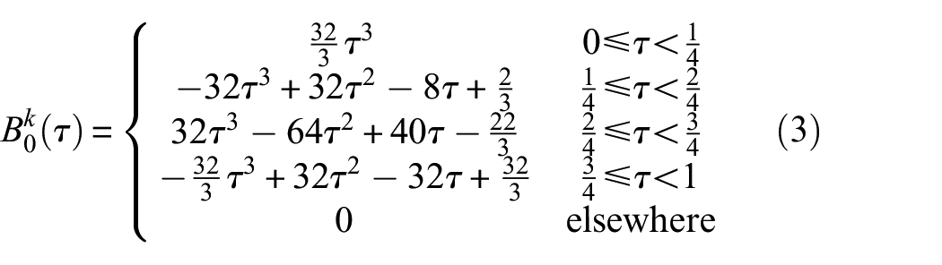
Any interpolation basis function may be used in a similar manner to the B-Spline polynomial. However, the B-Spline family of polynomials are chosen for this work due to the following attributes. B-Splines are defined based on a discrete knot sequence. Equally spaced knots of any length significantly simplify the computation effort and is consistent with data acquisition sampling practices. The choice of the time knot spacing serves as a natural filter of high frequencies of the interpolating polynomial and, by extension, of the resulting BSR. B-Splines can be of any order. Cubic B-Splines are the lowest-order basis functions that satisfy continuity requirements of fundamental principles in elastodynamics, that is, any source excitation has to be twice differentiable.35,44 Thus, the cubic B-Spline polynomial with equally spaced knots is chosen due to its flexibility and suitability in producing BSRs that capture complex structural responses without violating fundamental principles of the physics-based models.
To this end, the vector of arbitrary transient external excitations,
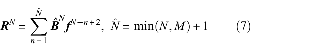
where step M defines the time
The inverse problem
The current state of the structure is captured in the BSR. Therefore, if the response time history,
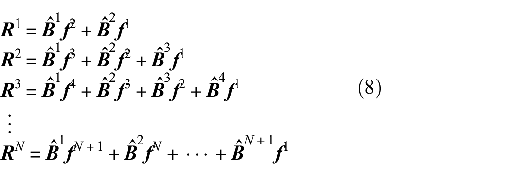
Equations (8) contain one more unknown than the number of equations and cannot be solved for in this form. The additional needed equation is obtained by assuming a natural condition for the BSR function at any step,
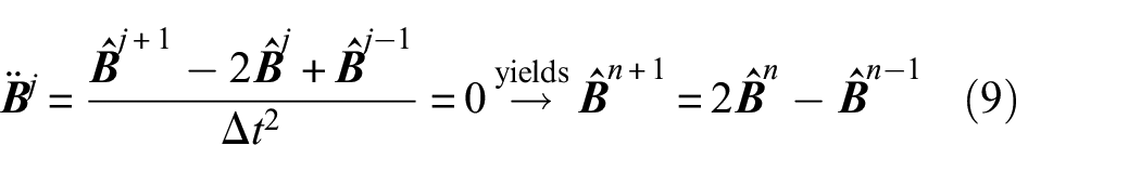
Introducing Equations (9) into (8) yields:
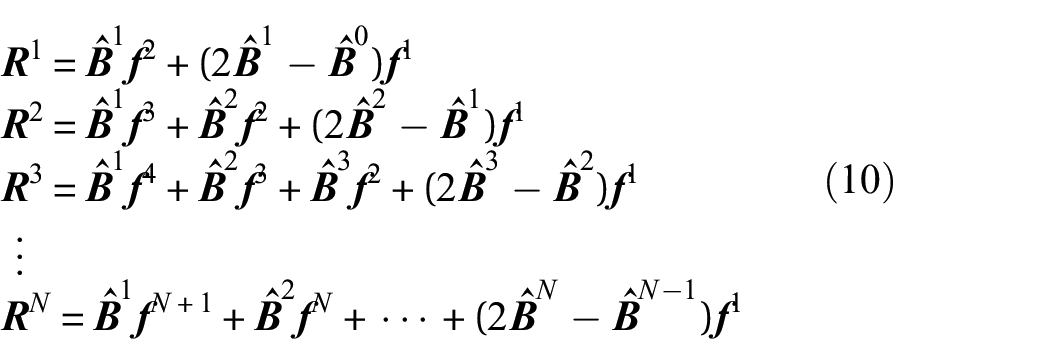
which in compact form can be written as
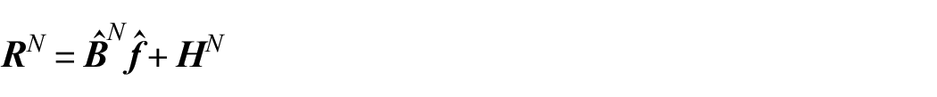
where

where
Numerical validation of BSR extraction
Multi-DOF system
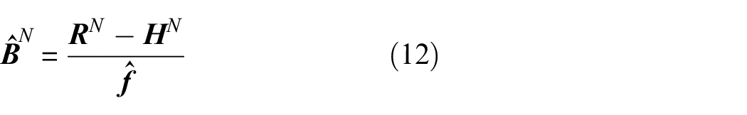
The proposed procedure for extracting the signature response is verified first using computer simulated system responses. For demonstration purposes, and without loss of generality, a two DOF system is considered as shown in Figure 3(a). The system parameters are given in consistent units as
System, loads, and representative response time histories: (a) 2-DOF system, (b) the three excitation time histories,(c) displacement response at DOF 2 due to excitations A, B, and C at DOF 1 and (d) acceleration response at DOF 2 due to excitations A, B, and C at DOF 2.
Extracting the BSR
With both the loading and responses known, Equation (12) can be used to extract the individual BSR components that make up the BSR matrix of the system. The BSR can be extracted using any type of response (displacement, velocity, or acceleration) measurement and is demonstrated for displacement and acceleration. This procedure is repeated for each combination of source and receiver to assemble the BSR matrix for both displacement and acceleration, which is examined in the following sections.
Displacement-based BSR
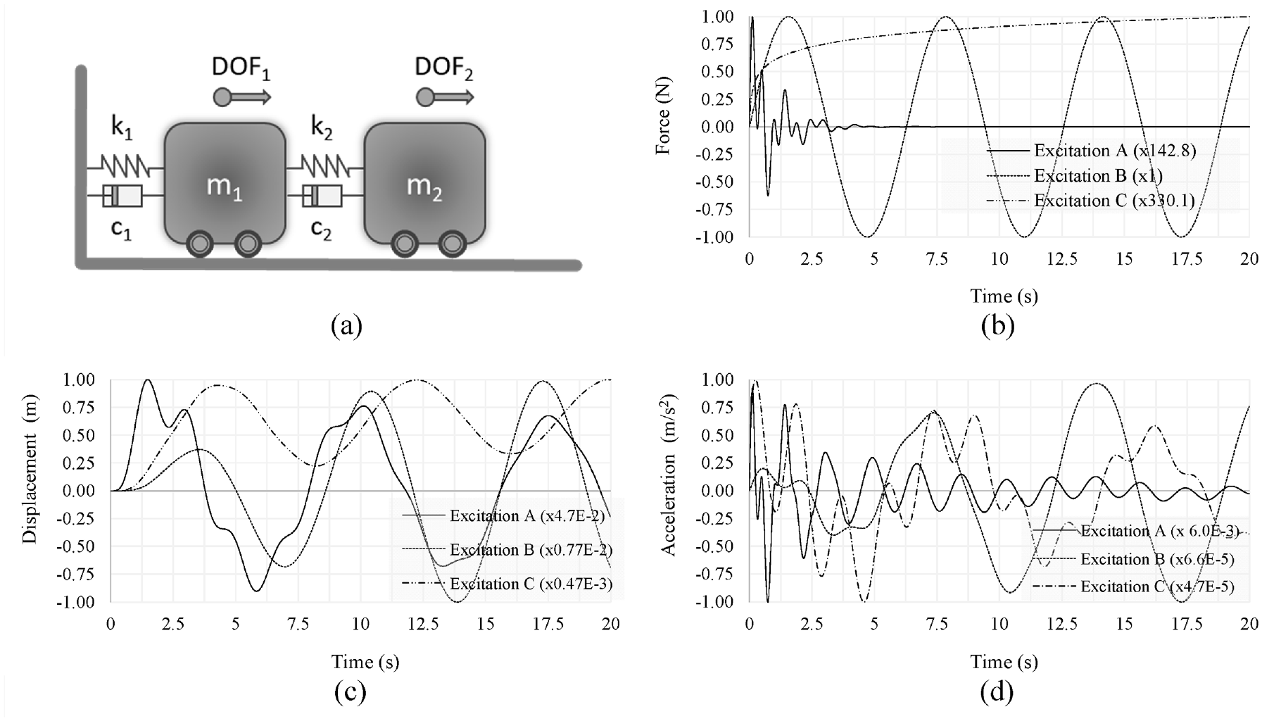
The loading and corresponding displacement responses are used in Equation (12) to extract the system’s displacement-based BSR. Since the system remains the same, it is expected that the signature responses would be identical when extracted from differing load cases, which is shown in Figure 4.
Extracted displacement-based BSR components from excitations A, B, and C.
Acceleration based BSR
Since acceleration measurements are easier to acquire in experiments, the same procedure shown above is used again here with acceleration-based BSR extraction. The extracted acceleration-based BSR from each excitation is shown in Figure 5. As expected, the signature responses are again identical regardless of the excitation.
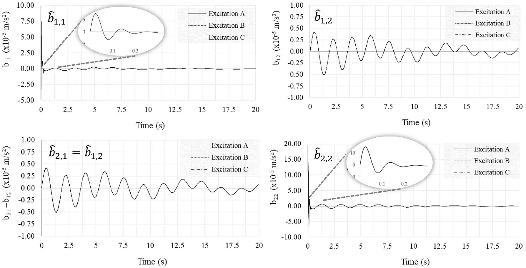
Extracted acceleration-based BSR components from excitations A, B, and C are indistinguishable from one another.
Using BSR to calculate system response to arbitrary loading
This section demonstrates that, without further consideration of the system itself, the extracted BSR can be used to calculate the actual response when any loading is known. To this end, DOF 1 of the system is subjected to the force excitation, Excitation D, as shown in Figure 6(a). The system responses are calculated in Equation (7) using this known excitation time history and the extracted BSRs (Figures 4 and 5). It is noted that only the first column of the BSR matrix that corresponds to the “excited” DOF 1 is needed in the summation shown in Equation (7). The system displacement, velocity, and acceleration responses of all DOFs are also independently computed using Abaqus and the solutions are compared. Figure 6 shows comparisons of representative solutions for the displacement and acceleration response. It is mentioned that the cross-correlation coefficients for the Abaqus generated and the BSR calculated responses are all 1.0000, verifying, thus, the excellent accuracy of the proposed methodology.
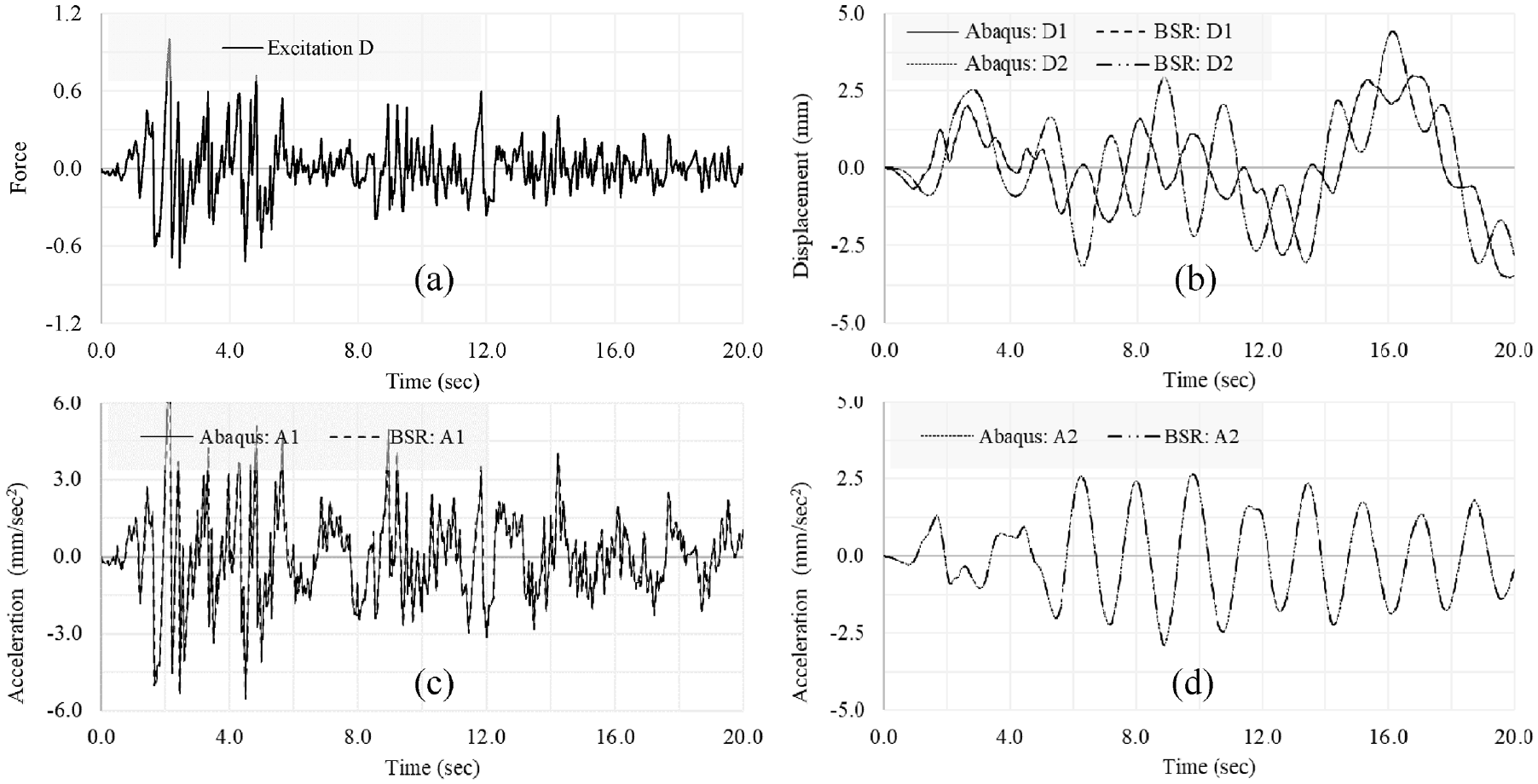
Verification study comparing Abaqus solution with BSR synthesis: (a) excitation time history at DOF 1, (b) displacement response history of DOF 1 and 2, (c) acceleration response history of DOF 1 and (d) acceleration response history of DOF 2.
Observations and checks
Response to arbitrary excitation
When any arbitrary force is applied to the system, the extracted BSR remains unchanged, as evidenced by Figures 4 and 5. This demonstrates how the BSR is independent of external excitation and is dependent solely on the system parameters. The BSR is unique to the current state of the structure.
Symmetry
It is observed that for both acceleration and displacement BSR,
Acceleration as second derivative of position
As acceleration is the second derivative of displacement, so too should the acceleration-based BSR be the second derivative of the displacement-based BSR. As an example of this mathematical check, the displacement-based BSRs,
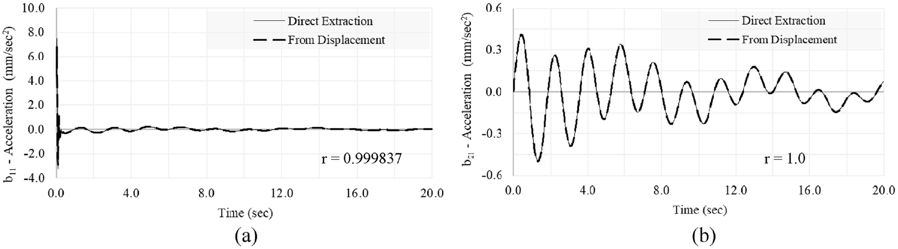
Comparison of extracted versus derived acceleration BSRs for (a)
Experimental validation of BSR extraction
Laboratory experiments were conducted to validate BSR extraction from physical structures. A cantilever structure was excited at various locations using a modal hammer and the acceleration time history was acquired through an accelerometer. The recorded time histories of excitation force and acceleration response were used to extract the BSR between source and receiver points.
Experiment setup
The physical parameters of the structure shown in Figure 8 are
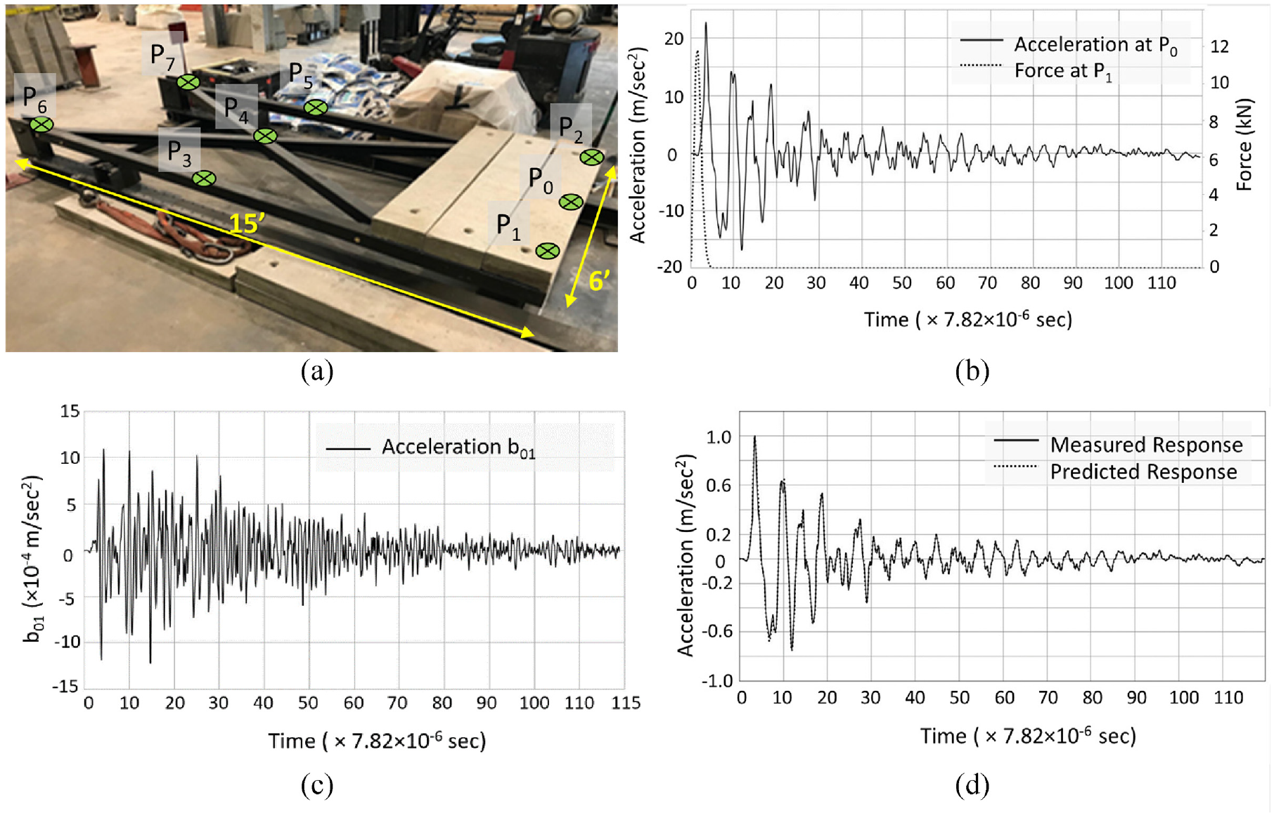
Experimental validation: (a) test structure and setup, (b) time histories of force applied at P1 and acceleration response measured at P0 for extraction of b01, (c) the extracted acceleration b01 using experimental data in b and (d) comparison of measured and predicted acceleration response at P0 when P1 is excited.
Testing procedure
Each test consists of a pair of points, one source point and one receiver point. The source points
The extracted BSRs are expected to remain the same between each point pair, independent of the applied load. To test this concept, the receiver is excited by a second hammer blow and the force and acceleration time histories again recorded. A comparison is then done between the recorded acceleration response to the second blow and the acceleration response predicted with the previously calculated acceleration BSR (from the first hammer blow) utilizing Equation (11). Consistent with notation, each signature response is denoted as b ij , where i indicates the receiver point and j indicates the source point.
Experimental validation study
Here, b01 is presented to demonstrate that signature responses can be extracted experimentally using load and response data and can be subsequently used to predict the response at a receiver point due to any load applied at the source. Figure 8(b) shows the initial force time history at the source node,
Finally, Figure 8(d) shows the acceleration response of the receiver node in response to a second hammer strike in comparison to the response predicted by utilizing the extracted acceleration b01. As expected, they are identical, which shows that the BSR is independent of the excitation and is a unique characteristic that depends on the state of the structure between the source and the receiver points. It is noted that similar behavior is observed for all source–receiver pairs in this experimental validation.
BSR change detection method
BSRs are unique to a structure and capture the state of the structure at the time of extraction without a need to quantify the individual physical structural parameters. The BSRs remain unchanged if the state of the structure is time invariant. The proposed concept for change detection takes advantage of the BSR invariance and identifies change through comparing BSR signals extracted at different points in the structure’s life. Taking one BSR as a baseline state, change is determined by measuring the deviation from the baseline BSR using an appropriate signal processing technique. In this study, change of any two BSR records of the same structure obtained at different times is detected through the cross-correlation coefficient of the records evaluated as
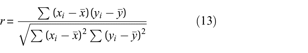
where
Correlation loss between two BSR signals indicates change in the state of the structure between the two acquisitions, which can be associated with damage, although correlation loss in general may be attributed to other factors such as quality of the acquisition. Structural changes detectable by the BSRs include alterations in geometric configuration, material properties, or boundary conditions, as well as the presence of damage or deterioration. These changes appear as deviations in the BSRs extracted at different points during the life of the structure, indicating changes in the dynamic behavior.
Numerical investigation of BSR change detection method
A numerical study using computer simulations was conducted to investigate how significantly a system must be changed before it will be detected by a poor signal correlation of BSRs. For this study, the two DOF system shown in Figure 3(a) is considered. The baseline structure is taken with the system parameters as
The efficacy of the proposed method was examined by correlating the BSR of the baseline system with the BSR of systems with progressively reduced stiffness. Stiffness reduction in one element at a time as well as both elements simultaneously was conducted, and acceleration and displacement BSRs was extracted for each case. Each individual BSR (b11, b12, b21, and b22) for every changed case is cross-correlated to the baseline case. Figure 9 shows how the BSR correlation coefficient reduces as stiffness degrades. It should be noted that the individual BSRs do not lose correlation uniformly. Table 1 quantifies the %Δ from the baseline case’s value for each variable and calculated value. The intent is to isolate change to only the stiffness. However, changing stiffness unavoidably changes the damping coefficient, as the damping ratio was left unchanged. These small changes in damping coefficients were noted to negligibly affect the BSR of the structure. Similarly, a changed stiffness causes a change in the natural frequencies. Within this table, poor correlation values (i.e., <0.90) are denoted in bold.
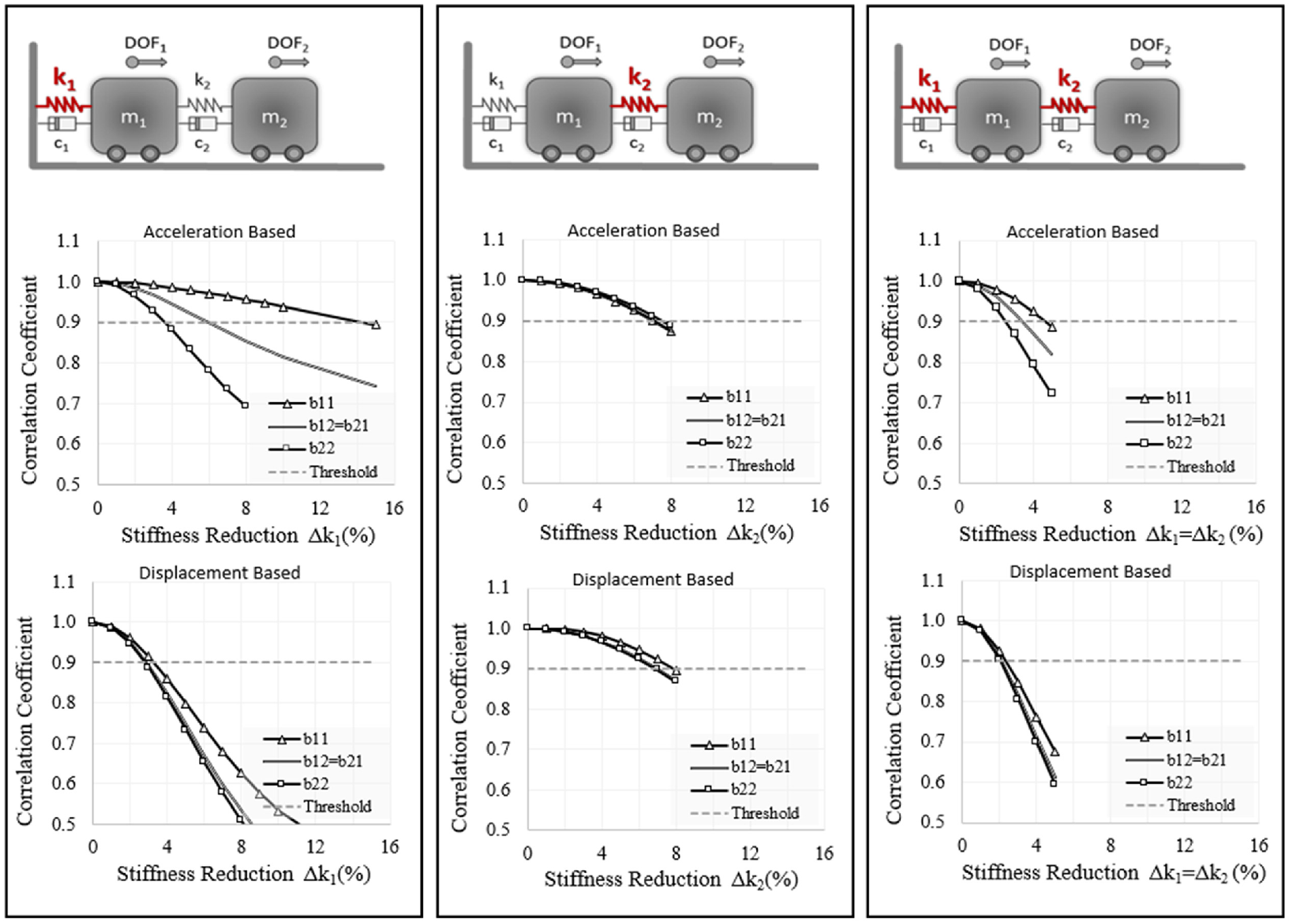
Loss of correlation of (a) displacement and (b) acceleration BSRs to baseline state as stiffness changes in a single DOF.
Percent change of parameter values for condition states with change in single DOF.
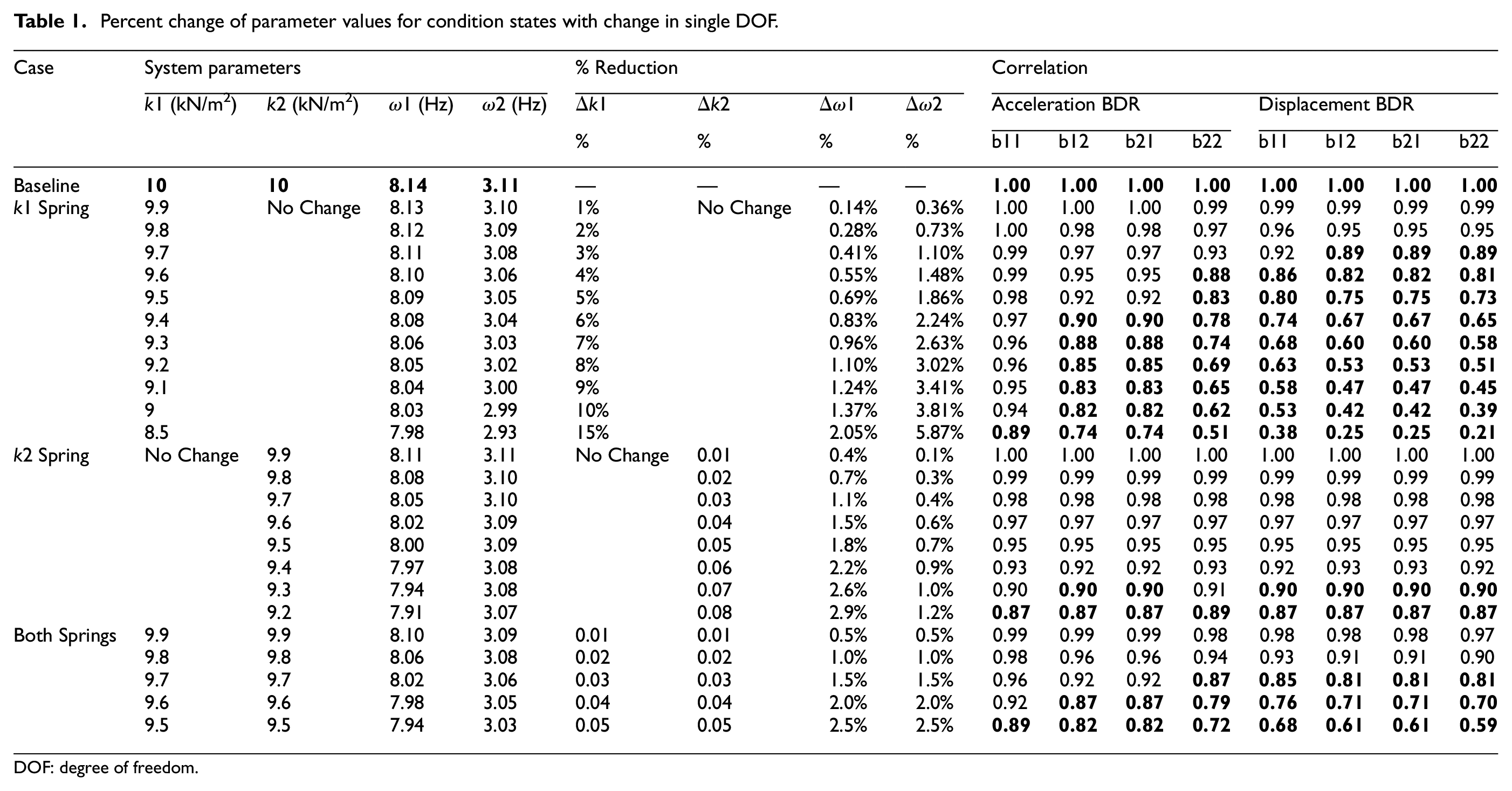
DOF: degree of freedom.
When change is located in the first DOF (spring k1), correlation is initially lost in one BSR for the displacement and acceleration BSRs at 3% and 4% loss in stiffness, respectively, and correlation is completely lost in all BSRs at 4% and 15% loss in stiffness for displacement and acceleration BSRs, respectively. With change in the second DOF (spring k2), correlation is initially lost for both displacement and acceleration BSRs at 7% loss in stiffness and completely lost in all BSRs at 8% loss in stiffness. These studies investigate the proposed method’s performance on singular, localized changes. The configuration of the system puts the first lumped mass in a constrained position, with both k1 and k2 restraining movement, while the second lumped mass is in a more unconstrained position, with the effects of the springs in series consolidated. The disparity between the first and second DOFs in magnitude of %Δ before change is detected indicates the BSR is in some way dependent on the system configuration and warrants further investigation. Additionally, the method appears to be more sensitive to changes in displacement than acceleration, which presents an opportunity for possibly implementing this change detection method with sensors that can detect deformation, such as digital image correlation.
When stiffness is reduced in both springs, a more widespread or global type of change with multiple locations of change is represented. For the displacement BSR, correlation was lost in all BSRs at the same time, at 3% loss in stiffness of both k1 and k2. For acceleration BSR, correlation was lost in one BSR initially at 3% stiffness loss and lost for all BSRs at 5%. It is important to note the distinctions in the BSR correlation values for each condition state.
Changes in BSR versus natural frequencies
The natural frequencies of the baseline case were selected to be representative of a typical structure. The %Δ in the natural frequencies was tracked for each condition case. Intriguingly, the natural frequencies of this system do not change significantly, between 0.5 and 2.5%, when the change in stiffness is initially detected by loss of correlation in the BSRs.
This highlights an important concept: that the natural frequencies can remain relatively unchanged in the presence of significant structural changes. This has been a point of struggle for some damage detection methods that rely on analyzing mode shapes or natural frequencies. The presented method is not reliant on natural frequencies, or quantifying any parametric value for that matter, and appears to be more robust to detecting small structural changes. There also exists the potential for structural change to occur in both stiffness and damping or mass that would cause the natural frequency to remain unchanged, masking the damage. The presented BSR method would be able to detect this change and will be examined in further studies.
Experimental validation of BSR change detection method
A laboratory experiment was conducted to validate the proposed change detection method. A steel plate was bolted to a braced steel frame, shown in Figure 10. The plate was harmonically excited to obtain an initial BSR. Bolts were then removed to introduce structural change and a secondary BSR of the changed structure was extracted for comparison to the initial BSR. Change was determined by poor correlation of the two signals. Details of this experiment were previously published within the context of the development and implementation of a drone-based vibration monitoring and structural assessment system.48,49 The proposed change detection algorithm for damage detection was implemented as the damage detection algorithm of the drone-based system and was introduced without a rigorous discussion of the fundamentals of the BSR techniques and the development and validation of the change detection algorithm, as was done here.
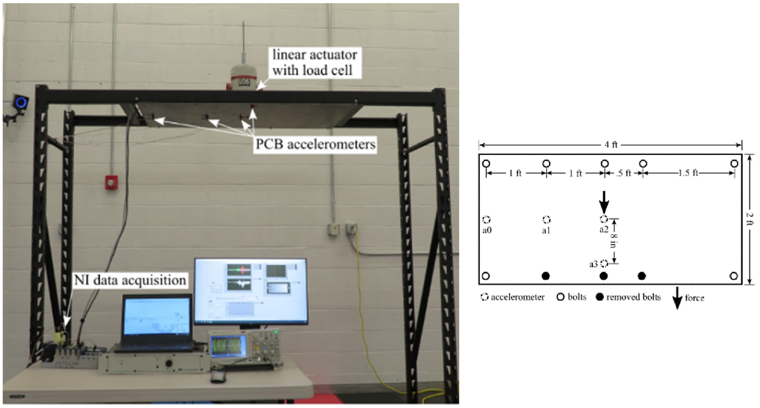
Structural change detection testing apparatus. 48
Experimental validation results
It is expected that any physical changes in the structure’s configuration will alter the BSR. This would be evident through signal correlation of the “before change” and “after change” signature responses. As an example, Figure 11 shows the extracted acceleration based BSRs of before and after instituting change via removal of bolts. The visually apparent differences in these BSRs are quantified in Table 2, which shows the averaged correlation coefficients across three tests. The high correlation coefficients between the three tests of before change supports the previously shown characteristics of BSRs as independent of input force and unique to the structure at the time of extraction. The same is true of the correlation between the three tests after change. However, there is a significantly reduced correlation between the before and after change signals, demonstrating how structural change is indicated by a loss of correlation.
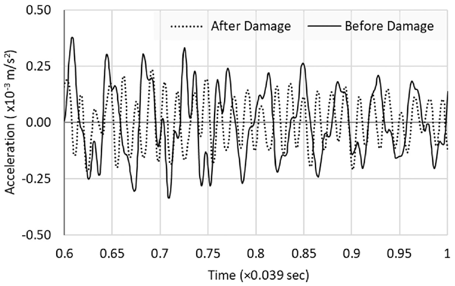
Acceleration-based BSRs of a structure before and after change.
Correlation of BSR before and after change (average cross-correlations of three tests).
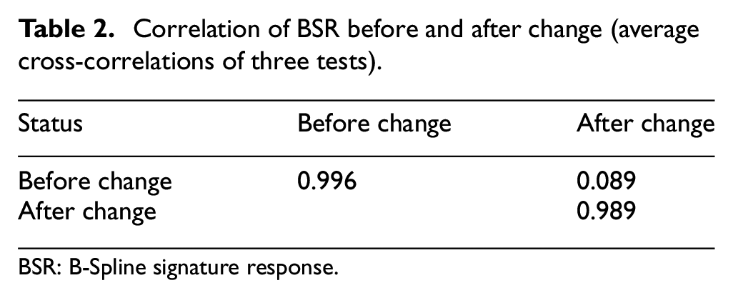
BSR: B-Spline signature response.
Conclusion
This study introduces the BSR concept within the framework of change detection and is intended to be the first in a series of work that expands the method to complement and improve on current SHM approaches. It has been demonstrated that the BSR captures in a single, discrete time domain, response function the combined effects of the system attributes on the response of the structure (“state” of the system), without explicitly quantifying the individual attributes a priori. BSR is independent of external excitations, and it forms a basis function of the system response to any external excitation. A single BSR, by itself, does not detect structural changes. Structural changes are identified as deviations of any BSR from its baseline. Because BSR captures the combined effects of all system attributes in a single function, the fundamental form of the BSR-based change detection presented in this work does not identify the source of the structural change (e.g., change in geometric configuration, material properties, or boundary conditions, as well as the presence of damage or deterioration). The proposed change detection method is successfully demonstrated in numerical studies and laboratory experiments. The findings of the studies presented in this article form the basis of current and future investigations on the development, implementation, and qualification of the proposed method to specific applications. In particular ongoing and future studies are addressing the following research questions:
The presented study establishes the fundamentals of the methodology and proof of concept, while setting the framework for further investigations focusing on (i) addressing specific application challenges, such as sensitivity to measurement noise and varying environmental or operational conditions; (ii) identifying potential benefits compared to existing techniques in view of the reduced data processing requirements of the BSR; and (iii) integrating with current SHM practices.
The BSR concept has been derived from linear systems. However, the application of BSR change detection may be extended to capture the dynamic responses of nonlinear systems and the BSR invariance would hold with the additional consideration of small perturbations. Experimental validation of this concept and development of testing procedures are in progress.
By definition, a BSR function relates excitation to response between any two locations and thus, the proposed change detection concept at its current development state detects the presence of change between these two points. However, localization and severity of the change detection can be determined through a coupled analysis of the spatial and temporal patterns of correlation loss between a network of point pairs. Global or local changes can be differentiated by defining an appropriate size and density of this network.
The BSR method will detect any changes of the intrinsic dynamic characteristics, including temporary changes such as those due to temperature fluctuations. While temperature is not an intrinsic characteristic itself, intrinsic characteristics of the system may be temperature-dependent, and significant temperature changes can alter the state of the system. The system may or may not return to its previous state once temperature effects subside. This warrants further investigations regarding the testing protocol to account for temporary system state changes.
Footnotes
Declaration of conflicting interests
The author(s) declared no potential conflicts of interest with respect to the research, authorship, and/or publication of this article.
Funding
The author(s) received no financial support for the research, authorship, and/or publication of this article.