
Abstract
Guided ultrasonic wave based structural health monitoring has been of interest over decades. However, the influence of prestress states on the propagation of Lamb waves in thin-walled structures is not fully covered yet. So far experimental work presented in the literature only focuses on a few individual frequencies, which does not allow a comprehensive verification of the numerous numerical investigations. Furthermore, most work is based on the strain-energy density function by Murnaghan. To validate the common modeling approach and to investigate the suitability of other nonlinear strain-energy density functions, an extensive experimental and numerical investigation covering a large frequency range is presented here. The numerical simulation comprises the use of the Neo-Hooke as well as the Murnaghan material model. It is found that these two material models show qualitatively similar results. Furthermore, the comparison with the experimental results reveals that the Neo-Hooke material model reproduces the effect of prestress on the difference in the Lamb wave phase velocity very well in most cases. For the
Keywords
Introduction
A promising method for the development of reliable structural health monitoring (SHM) systems for lightweight structures utilizes guided ultrasonic waves (GUWs). Based on their propagation characteristics and interactions with discontinuities in the waveguide, information about material properties or existing damage in the material can be obtained.1,2 In order to analyze the wave propagation data correctly, knowledge about the fundamental wave propagation properties and the influences of structural properties, damage, inhomogeneities, and environmental conditions is indispensable. Furthermore, the presence of internal stresses and strains leads to a change in the phase velocity of GUW propagating in solids. This phenomenon is known as the acoustoelastic effect.3,4 Since all structures are subject to gravity and hence exhibit internal stress states at any time, the interaction of GUW with stress states is crucial for an accurate interpretation of the measurement data.
Fundamental investigations in the field of acoustoelasticity go back to geophysical problems. Biot5,6 developed a theory for the analysis of small deformations and elastic waves under the influence of an internal stress state. Based on this the influence of an internal stress state on homogeneous plane waves can be found in Man and Lu. 7 In the field of acoustoelasticity it is initially not relevant what causes the internal stress state. However, two different scenarios can be distinguished. If the internal stress state is present in the absence of loads, it is referred to as a residual stress state. 8 Otherwise, it is referred to as a prestress state.
More recent studies in the field of acoustoelasticity rely on nonlinear constitutive models to describe the occurring effects. In the field of solid mechanics, and especially in the field of GUW-based SHM, the application of constitutive models to represent the acoustoelastic effect is limited to the strain-energy density function introduced by Murnaghan. 9 This is based on the work of Hughes and Kelly, 10 which deals with the experimental determination of third-order elastic constants by investigating the wave propagation in isotropic materials under the influence of uniaxial and hydrostatic stress states. Thurston and Brugger 11 as well as Toupin and Bernstein 12 extended these investigations to materials with arbitrary crystalline symmetries. Among others Crecraft, 13 Hsu 14 as well as Blinka and Sachse 15 were able to determine the elastic stress states in solids using longitudinal and shear waves. For an overview of the theory of acoustoelasticity and also acoustoplasticity with a focus on hyperelastic anisotropic materials using Murnaghan’s constitutive theories, the reader is kindly referred to Pao and Gamer, 3 Guz and Makhort, 16 and the sources therein.
Early studies on acoustoelasticity in the field of GUW can be found in the works of Hayes 17 and Husson, 18 which provide formulations for the modeling of the acoustoelastic effect. Recent literature contains a large number of numerical studies on this topic using a wide variety of geometries and materials.4,19–25 However, literature dealing with the validation of numerical and analytical results by experimental data is very limited. Gandhi et al. 26 investigate the acoustoelastic effect by measuring the wave velocities of Lamb waves in biaxially stressed plates and compare the results with analytical results. Qiu et al. 27 investigate the influence on wave propagation for uniaxially prestressed plates with a focus on numerical multiphysics simulations considering piezoelectric transducers. Pei and Bond 28 deal with the influence of residual stress states on the propagation behavior of Lamb waves and the influence of uniaxial prestress states on higher-order modes. The listed work is limited to the consideration of the acoustoelastic effect at a few individual frequencies.
Furthermore, even if the field of acoustoelastic investigations in solids is limited to the strain-energy density function introduced by Murnaghan, a large number of other nonlinear constitutive theories are available in the literature. Therefore, in this work, the Neo-Hooke material model is additionally investigated, which goes back to the work of Ronald Rivlin29,30 and represents a classical extension of Hooke’s law to finite deformation elasticity. Further constitutive models for the representation of initial stress states were primarily developed within the field of biomechanics, where the focus is on residual stresses. Since the present work focuses on the influence of a prestressed state, the reader is kindly referred to the work of Ogden30–32 and Hoger8,33 and the sources contained therein for more details about residual stresses.
The state of the art described above highlights open research questions and motivates this work, namely the extension of the experimental investigations on the acoustoelastic effect to a large frequency range, comparative computations based on the Murnaghan and Neo-Hooke material models in the context of acoustoelastic problems, and the corresponding verification. Based on this the present study holds a comprehensive investigation of the influence of an uniaxial prestressed state on the GUW propagation in an isotropic waveguide. Therefore, first experiments are conducted to observe the acoustoelastic effect over a large frequency-thickness range of up to 3 MHz mm. For the data acquisition and evaluation, a technique is used, which was introduced by the authors in previous work.34,35 In the second step, numerical simulations are carried out. Here, not only the material model of Murnghan but also the well-known Neo-Hooke material model is used to incorporate the acoustoelastic effect. Using a small segment of the prestressed waveguide and following an approach presented by the authors in previous work, 36 again the acoustoelastic effect is studied over a frequency-thickness range of up to 3 MHz mm for both material models. To evaluate the numerical simulation and, hence, the suitability of the different material models, the obtained numerical data is compared with the experimental results in final step.
Subsequently, the structure is as follows. First, the theoretical fundamentals of the acoustoelastic effect are presented. Next are the experimental investigations on how prestress states influence the wave propagation properties in an aluminum strip specimen. This is followed by numerical simulations. Afterward, the experimentally obtained data is compared to the results of the numerical simulations based on the Neo-Hooke and Murnaghan material models. The presented work closes with a brief summary and conclusion.
Fundamentals
Investigations on prestressed hyperelastic structures require a revisiting of the theoretical foundations, such as the balance of linear momentum and the constitutive equations. This is the subject of this section.
Kinematics
The starting point of the investigations is the decomposition of the total deformation of the body

Here,
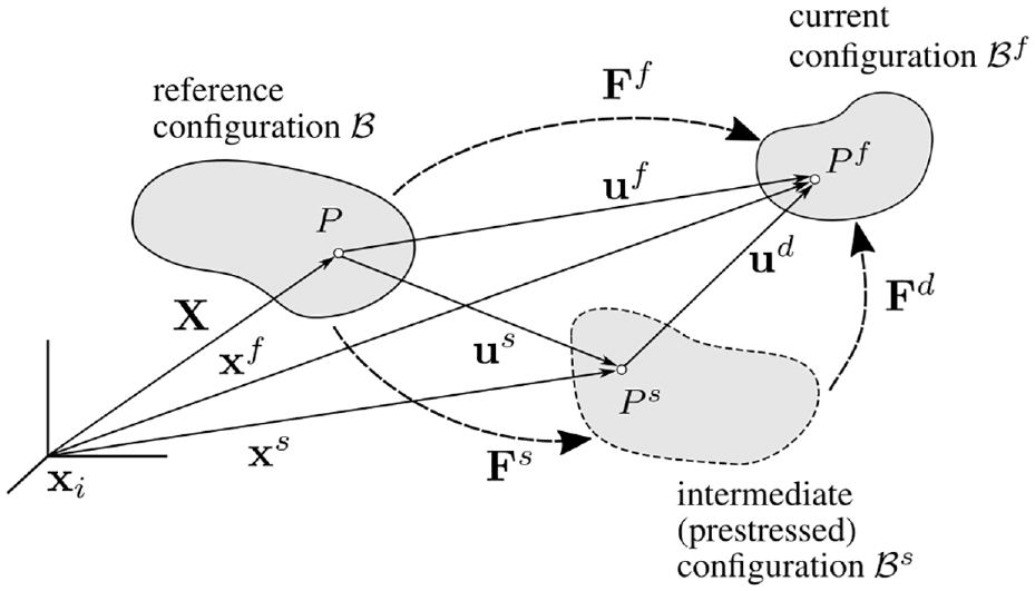
Sketch of configurations, position vectors, displacements, and deformation gradients.
Balance of linear momentum
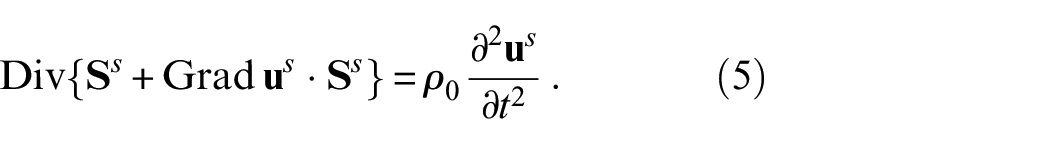
Next, the balance of linear momentum in the current configuration
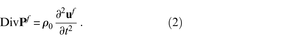
Here,
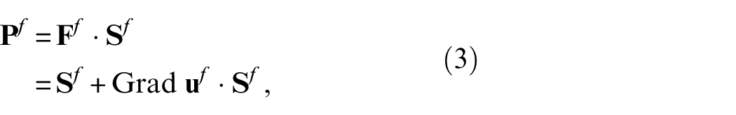
where
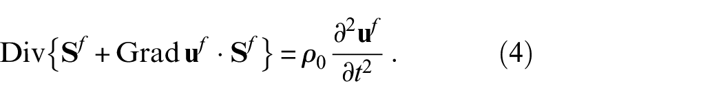
Analogously, the equation of equilibrium in the intermediate configuration
Subtraction 23 of Equations (5) from (4) yields
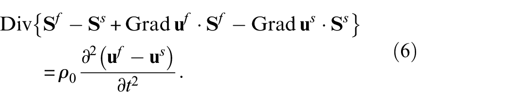
Now

and

After some rearrangements and by use of
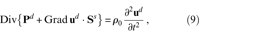
which is considered as the strong form of equilibrium of a body under prestress
Hyperelastic material models
In this work, it is assumed that the structures under consideration can be described by a hyperelastic material law. Then, a strain-energy density function W, which depends on the deformation gradient
When analyzing acoustoelastic phenomena, the Murnaghan material model9,37 is often used, for example.18,23,38 In terms of the invariants
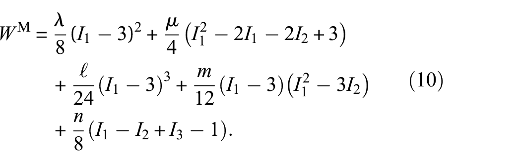
Here
A more easily applicable strain-energy function, often used in nonlinear elasticity, requiring only both Lamé constants, is associated with the Neo-Hooke material model. In case of a compressible material
In this work, the use of the Neo-Hooke material model is motivated by the fact that the prestress may cause a finite deformation, moving the reference configuration to the intermediate configuration and resulting in a deformation-dependent elasticity tensor. The subsequent infinitesimal deformation generated by the elastic waves, however, can be analyzed by a linearized theory in the intermediate configuration.
In the literature, see, for example, 30 further hyperelastic material models can be found, see for example, those according to Mooney-Rivlin or Yeoh. However, investigations on these models are beyond the scope of this work.
Experimental investigations
This section deals with the experimental investigation of the acoustoelastic effect in a prestressed aluminum strip specimen. Therefore, first the experimental setup is described before presenting the obtained results. With this data at hand, the numerical modeling approach, presented in the subsequent section, is validated in a last step by comparing it with the measurement data.
Methodology and procedure
For the observation of the GUW propagation the scanning laser vibrometry is a suitable technique.40–42 This allows one to measure the velocity component of the wave field that is parallel to the laser beam on the surface of a specimen. The result is a velocity matrix
To be able to analyze the effect of a prestress state on the wave propagation by also addressing the multimodal and dispersive nature of GUW, the postprocessing procedure focuses on the frequency-wavenumber domain. This also allows the use of a multifrequency excitation signal. Therefore, a superposition of sinusoidal oscillations is applied in this work. To avoid any influence by a finite sinus burst a Hann window is added. 48 The distance between the excited frequencies is set to 5 kHz. The raw signal can be described by the following expression
where
where M is the window width and m the index with
By repeating the measurement 40 times with an excitation signal shifted by 0.125 kHz the frequency resolution is significantly increased. Figure 2 gives an exemplary excitation signal in the time and frequency domain. It covers a frequency range from 0.125 to 995.25 kHz with steps of 5 kHz and has a total length of 80 ms. To illustrate the frequency resolution more in detail the frequency range on the right side in Figure 2 is reduced. Details regarding the extraction of the frequency—wavenumber pairs and the corresponding peak-search algorithm, as well as the identification of outliers, can be found in previous work by the authors.34,35
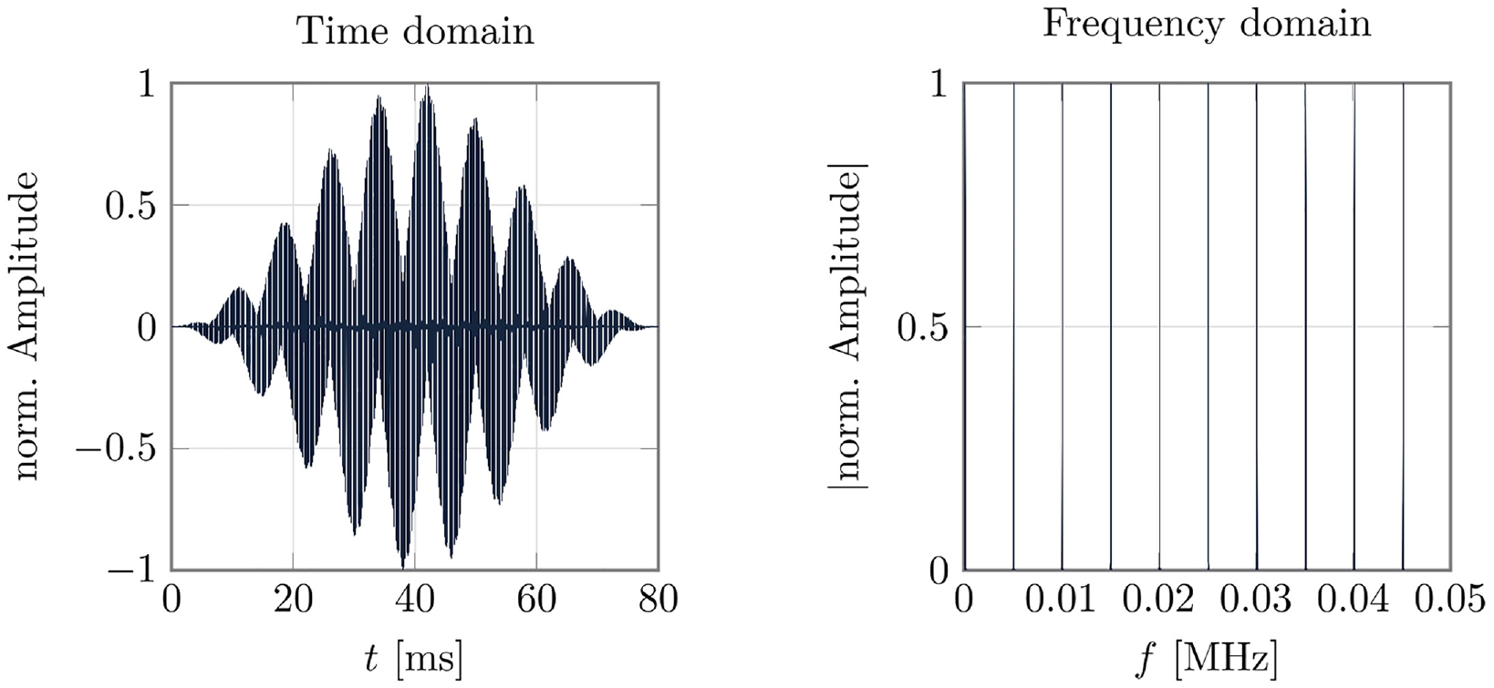
Multifrequent excitation signal. (1) Specimen D05-A, (2) Tensile test machine Z050SE, (3) Laservibrometer PSV500, and (4) Specimen grip 8455.
Within this work, the influence of a prestress state on the GUW propagation in aluminum is analyzed in a range from 0 MPa up to 100 MPa. Following this, the wave propagation is measured first in an unloaded specimen before increasing the external load by 10 MPa steps until a stress state of 100 MPa is reached. For each configuration, the measurement is repeated 40 times following the definition of the excitation signal. Furthermore, with respect to the designated wavenumber range a maximal excitation frequency of 1 and 2 MHz is used, respectively.
Setup and specimen definition
To measure the wave propagation in prestressed specimens, the waveguide is mounted vertically in a tensile test machine Z050SE, as depicted in Figure 3. The excitation signal is first amplified by a high-voltage amplifier before it is passed to a piezoelectric actuator, which is bonded to the surface of the specimen and excites the wave field. A rectangular piezo-ceramic actuator (ceramic type: PI Ceramic PIC 255) with the dimensions 30 × 5 × 0.2 mm3 is used. This shape results in a fairly straight wavefront along the measurement path. The actuator has a wrap-around electrode for one-sided access to the wiring. It is bonded onto the specimen’s surface with Loctite adhesive. The resonance frequencies can be derived from the frequency constants which are given by the data sheet
49
with
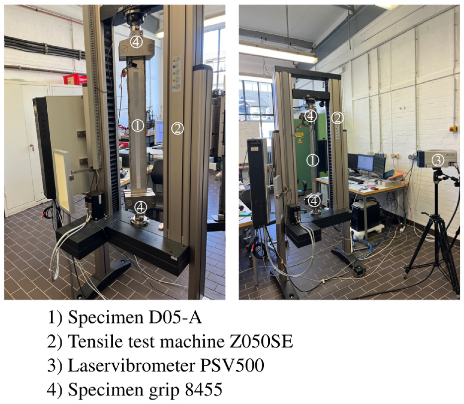
Experimental setup for the laser vibrometer measurement of the wave propagation in a prestressed specimen.
Furthermore, the size of the grips limits the specimen width. To ensure a mostly homogeneous stress field within the specimen, the grip size of 110 mm is identical to the width of the specimen. Due to the use of a non-uniform 2D-DFT for the data extraction and an additional damping on the specimen’s edges by plasticine the effect of edge reflections can be reduced significantly. 34 The length of the specimen is limited by the test area height. This leads to a specimen size of 1100 × 110 mm. Figure 4 depicts a strip specimen made from aluminum AlMg3. Based on the clamping length of the grips and the area required for the piezoelectric element, the maximum measurement length is 700 mm.
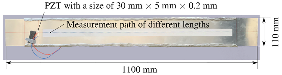
Strip specimen made from AlMg3 with a size of 1100 × 110 × 0.5 mm.
Lastly, the specimen thickness is directly linked to the desired frequency and wavenumber range of the obtained dispersion diagrams by the dispersion relation. Due to the Nyquist criterion with respect to time and space as well as the maximum resolution of the measurement path the observable wavenumber and frequency range are limited. 50
The minimal distance between two measurement points determines the maximum wavenumber. Following the Nyquist criterion, the highest wavenumber is given by half the spatial sampling rate. 34 Furthermore, in previous work of the authors, it was shown that there should be twenty full wave cycles along the measurement distance, 35 which gives the minimum wavenumber. Following this, the minimal and maximal wavenumbers can be obtained by
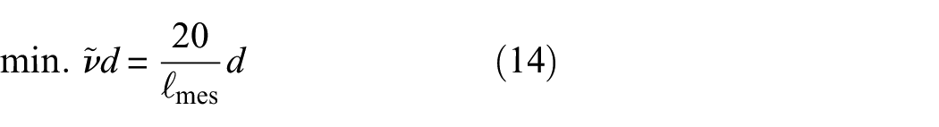
and
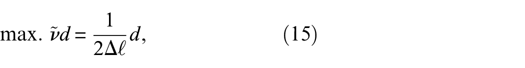
respectively. The variables are defined in Table 1.
Specimen specification.
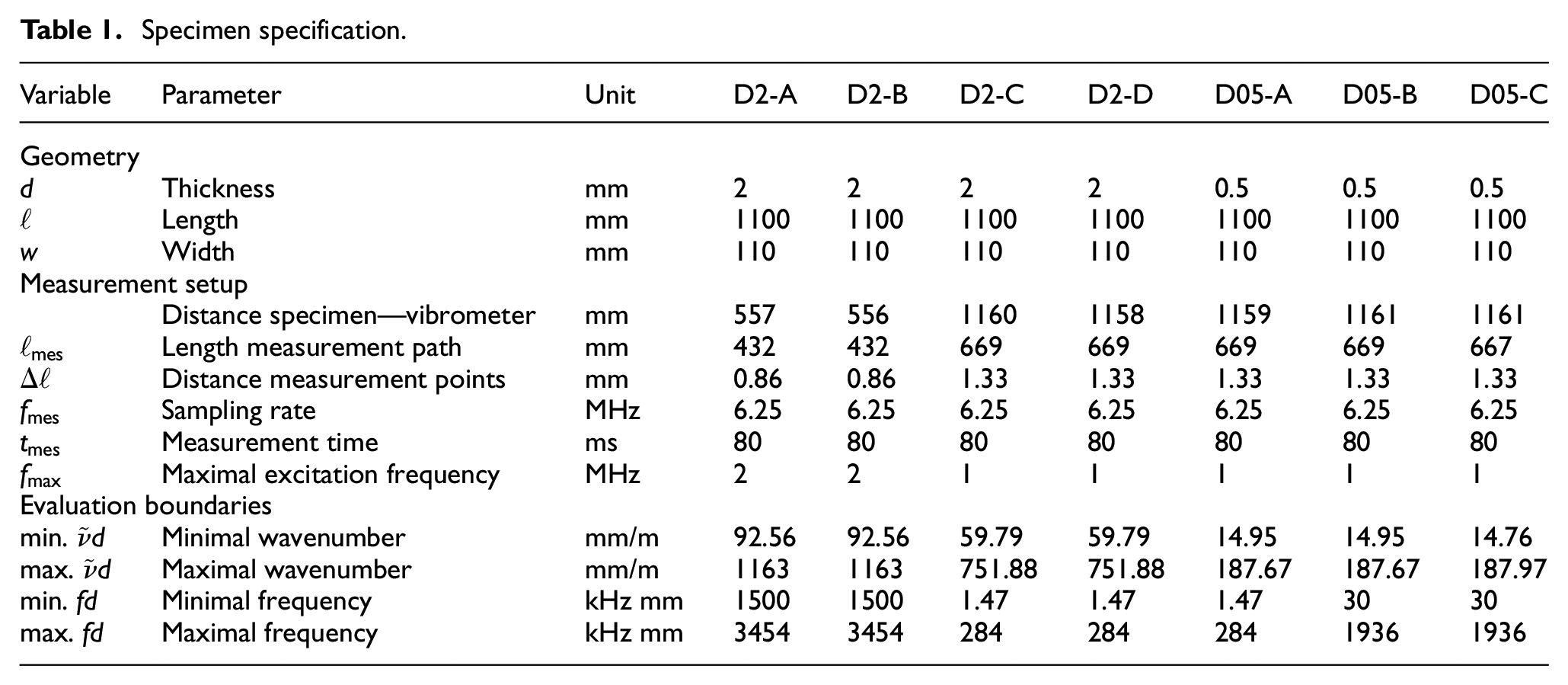
Based on the obtained wavenumber boundaries, the corresponding frequency range can be derived by solving the analytical framework of GUW. With a specimen of 2 mm thickness the
Results and discussion
In this section, the results of the experimental investigations are presented. To analyze the influence of prestress states on the wave propagation the difference of the phase velocity at certain frequencies is derived from the measurement data for each load step. The phase velocity difference
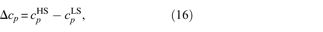
where the index

For the sake of clarity, Figure 5 only holds the change of the phase velocity for the
Phase velocity difference
The diagrams for both wave modes and all specimens indicate similar behavior. First, the measurements of the wave propagation in different specimens lead to comparable results. For the
Considering the influence of a stress state on the
The results are supported by the observation of the
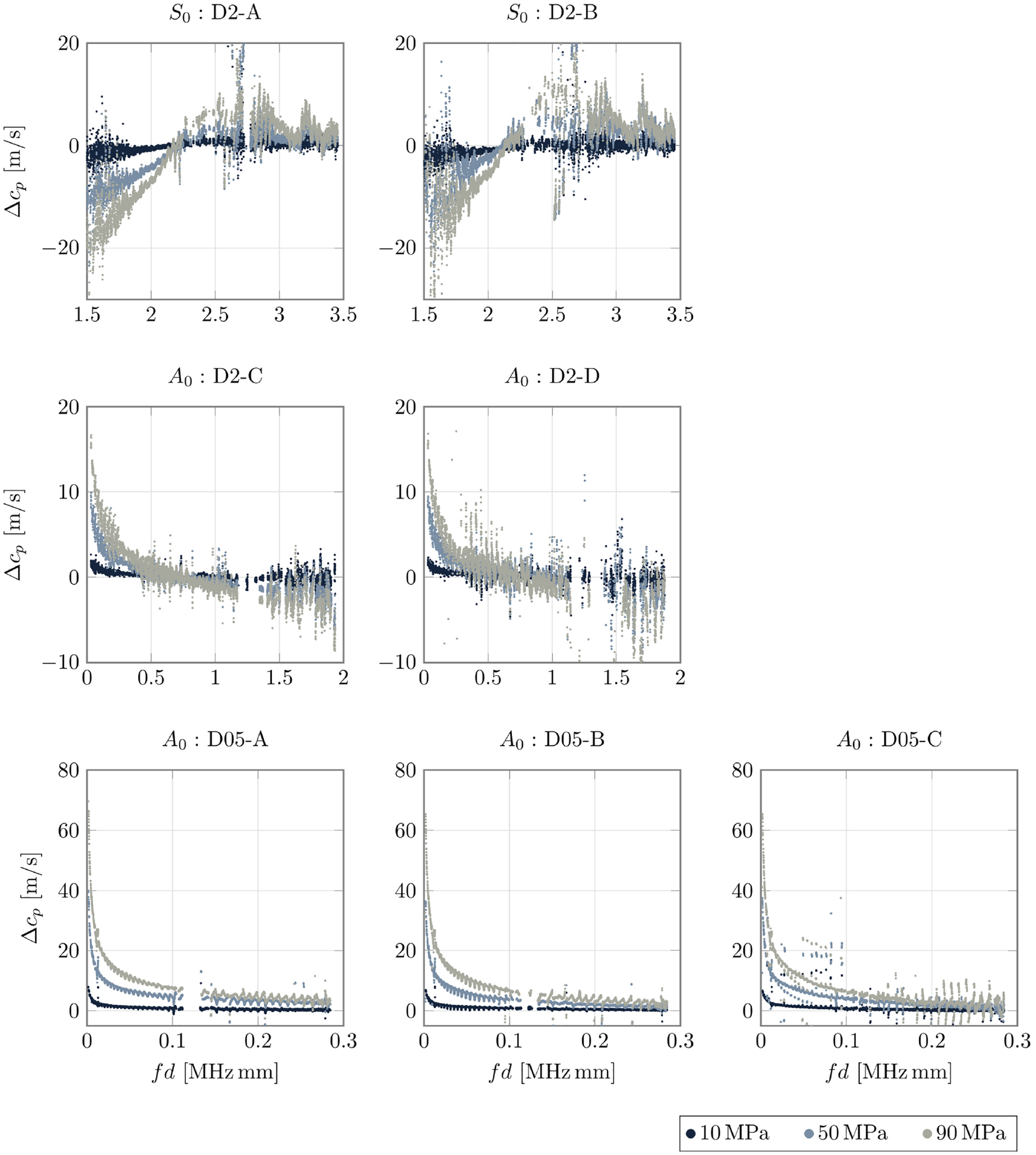
Based on the presented data it is the authors’ intention to analyze the correlation between the phase velocity difference and the prestress state more in detail. Thereby, special emphasis is laid on the
Approximation of the phase velocity
The first row of Figure 6 shows the comparison between the measured data and the regression curve for a frequency-thickness product of 50 kHz. The plots clearly indicate a linear relation between an increasing load state and an increase in the phase velocity for all three specimens. In the second row, this relationship can also be clearly concluded for a frequency-thickness product of 100 kHz. However, with an increasing frequency, the deviation between the measurement data and the linear regression increases. This can be observed in the last row, where the data is depicted for a frequency-thickness product of 200 kHz. Although the data still indicate a linear regression, this can no longer be clearly confirmed. This conclusion is mostly driven by the decreasing phase velocity difference due to a prestress state at higher frequencies, as shown in Figure 5, and is also linked to a decreasing value of
Numerical investigations
The finite element method is used for numerical analysis of the dynamically loaded prestressed specimens. However, before the computations are carried out, the weak form of equilibrium has to be formulated from Equation (9) and then linearized.
The computation of wave propagation in prestressed structures is carried out in a two-step procedure. First, the structure is loaded by external forces or a prescribed displacement, resulting in internal pre-stresses and accompanied by a mapping from the reference to the intermediate configuration, see Figure 1. Subsequently, the dynamical loads which are applied harmonically for the generation of the elastic waves are considered. They cause a mapping from the intermediate to the current configuration. To determine dispersion diagrams a linear eigenvalue problem is solved.
Weak form
The weak form of equilibrium is obtained by multiplying Equation (9) with the virtual displacement vector
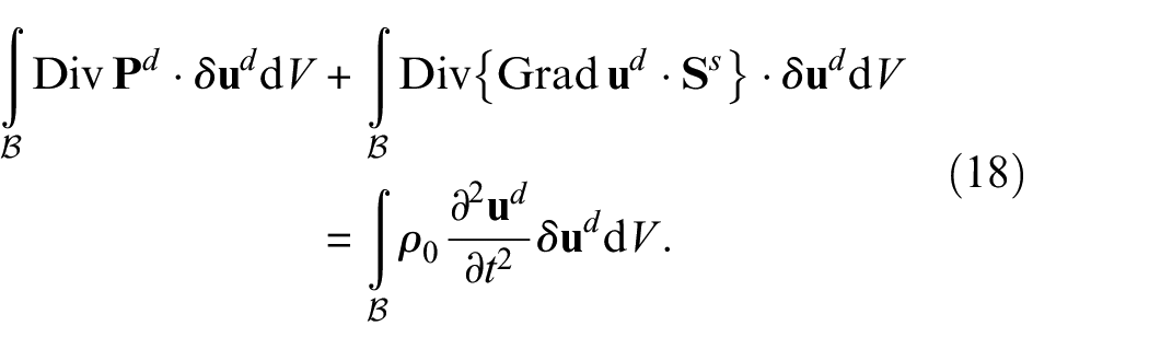
Further straightforward rearrangements by use of the product rule and the divergence theorem yield
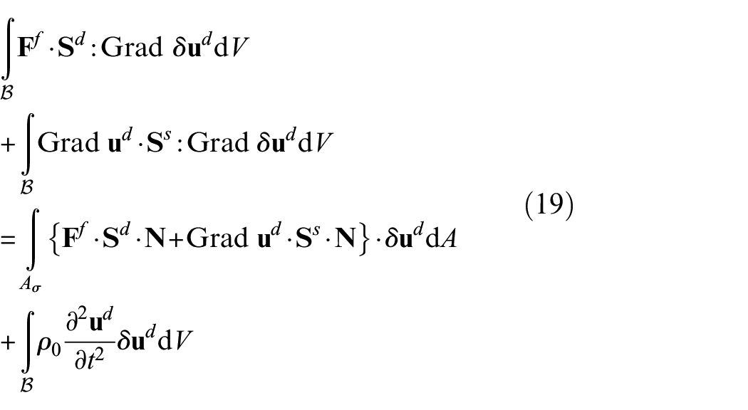
The two expressions on the left-hand side represent the virtual work of the internal stresses, while the virtual work of the external and the inertia loads appear on the right-hand side. Again, the standard formulation for the stress-free body is obtained for
Linearization
Equation (19) is nonlinear with respect to the displacement vector
Discretization and introduction of the standard finite element notation results in the following matrix equation for the entire system

Here,
Eigenvalue problem
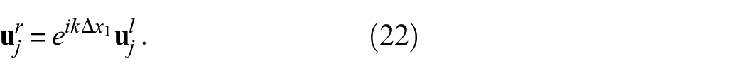
The following considerations are made with regard to isotropic strip-shaped waveguides, see Figure 4, but can easily adapted to other specimens. A corresponding model is shown in Figure 7. The nodal displacements

Here,
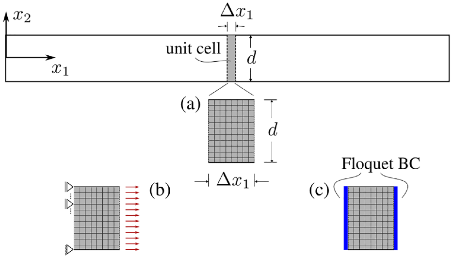
Scheme of specimen and discretized unit cell, not to scale (a), loading and boundary conditions for prestress analysis (b), Floquet boundary conditions (BC) for eigenvalue problem computation (c).
In this way, Floquet boundary conditions are formulated,53,54 which become conventional periodic boundary conditions for
Implementation of Equations (22) and (23) into Equation (20) and some subsequent rearrangements define the matrices

The computed eigenfrequencies are the circular frequencies
This method was originally intended for periodic waveguides but can also be used for homogeneous ones.54,55 It is effective and computationally efficient, especially for prestressed waveguides, since it can be employed directly with a general-purpose finite element code once the prestress state has been computed. In contrast to the semi-analytical finite element (SAFE) method,56–59 which assumes a displacement solution and requires the discretization of the cross-section of the waveguide, the present method uses a geometric assumption of the waveguide, for example, its periodicity, which is reflected by the boundary conditions. 53
Numerical model and computational procedure
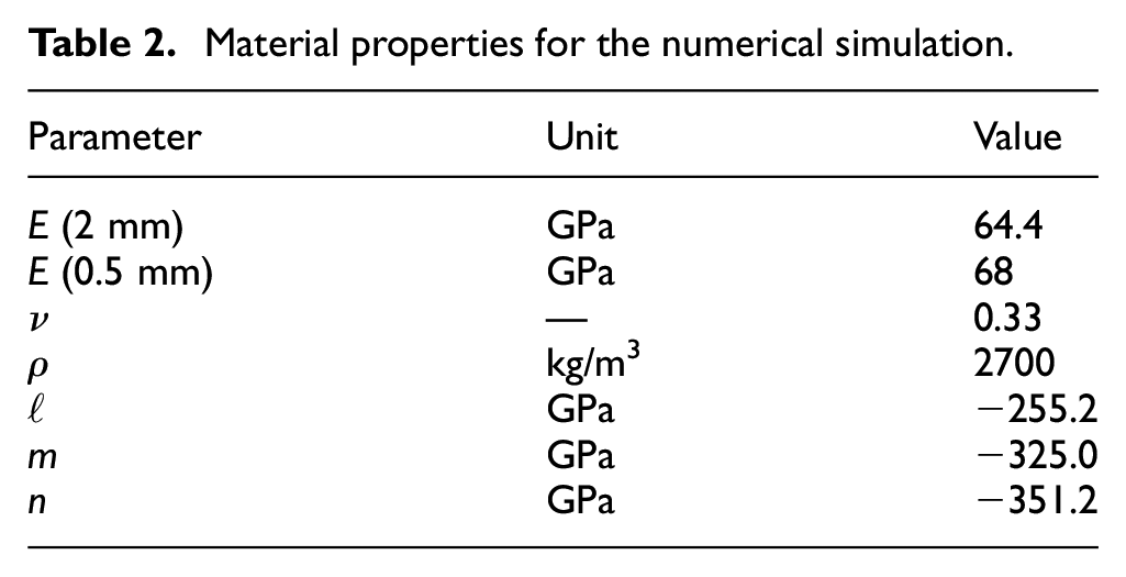
To simulate the acoustoelastic effect in an isotropic waveguide, a 2D model is created representing the specimen in Figure 4. The material properties of the numerical model are provided in Table 2. The Young’s modulus of the aluminum AlMg3 is experimentally obtained from the specimens used for the experimental investigation in section “Experimental investigations.” It is worth noting that Young’s modulus depends slightly on the specimen’s thickness. This will be considered when comparing the numerical and experimental results later on. The third-order elastic constants are taken from literature. 60 They are derived from acoustoelastic analyses based on the fatigue behavior of EN AW-7075. Even though this alloy differs slightly from the one used in the present study, this source is the best available in the literature for third-order elastic constants.
Material properties for the numerical simulation.
The finite element model maps the
The discretization is carried out using finite elements with biquadratic shape functions and a length of 0.01 mm, so that a total of 1000 elements are used. In Mace and Manconi, 61 Ichchou et al., 62 it is recommended to use at least 6 elements per wavelength and 10 nodes per wavelength for high spatial resolution. This means that the finite element mesh is very fine in relation to the expected wavelength, even in the high-frequency range. However, the finite element mesh of the unit cell only has a small number of degrees of freedom, so the computational time is short.
First, this finite element model is used to compute the prestress due to external loading in a standard nonlinear static analysis, see Figure 7(b). Here, either the Neo-Hooke or Murnaghan material model is used. The boundary conditions correspond to those in a common tensile test. The results of this computation are the mechanical quantities of the intermediate configuration.
The subsequent computations simulate the wave propagation in the specimen and yield the mechanical quantities in the current configuration. As mentioned above, a linear eigenvalue problem is solved for this purpose. The left and right boundary conditions now reflect the Floquet periodicity and thus allow the calculation on a unit cell that repeats periodically in the
Numerical results
Results of the numerical procedure for the characterization of the wave propagation in linear waveguides, especially the adapted eigenfrequency analysis to COMSOL Multiphysics, can be found in previous work of the authors.36,63 So, the focus of this subsection is on numerical investigations of prestressed structures.
Figure 8 shows the result of computations on the non-loaded and loaded strip-shaped specimen from Figure 7. The differences in the phase velocities when using linear and both hyperelastic material models in the range of the frequency-thickness product from 0 to 4 MHz mm are shown. As expected, the linear material model makes no difference between non-loaded and loaded specimens. However, both hyperelastic material laws are able to represent phase velocity differences under load, which here is 100 MPa. It is worth noting that both the Murnaghan and Neo-Hooke curves have a zero crossing, albeit at different modes.
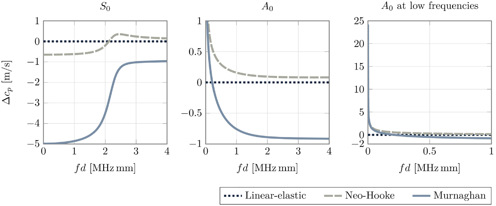
Phase velocities differences
In addition, computations are carried out on strip-shaped specimens at increasing pre-stresses from 0 to 100 MPa. In Figure 9, the results are presented for frequency-thickness products of 50 kHz mm and 3 MHz mm for both modes. It becomes obvious, that the results for the phase velocities at different prestress levels can be perfectly connected by a straight line for both material models and at both frequencies under consideration so that a linear dependency can be concluded. Figure 9 also shows that at the lower frequency, both material models have the same tendency, namely decreasing phase velocity with increasing prestress. However, at a higher frequency, the two material models show opposite behavior.
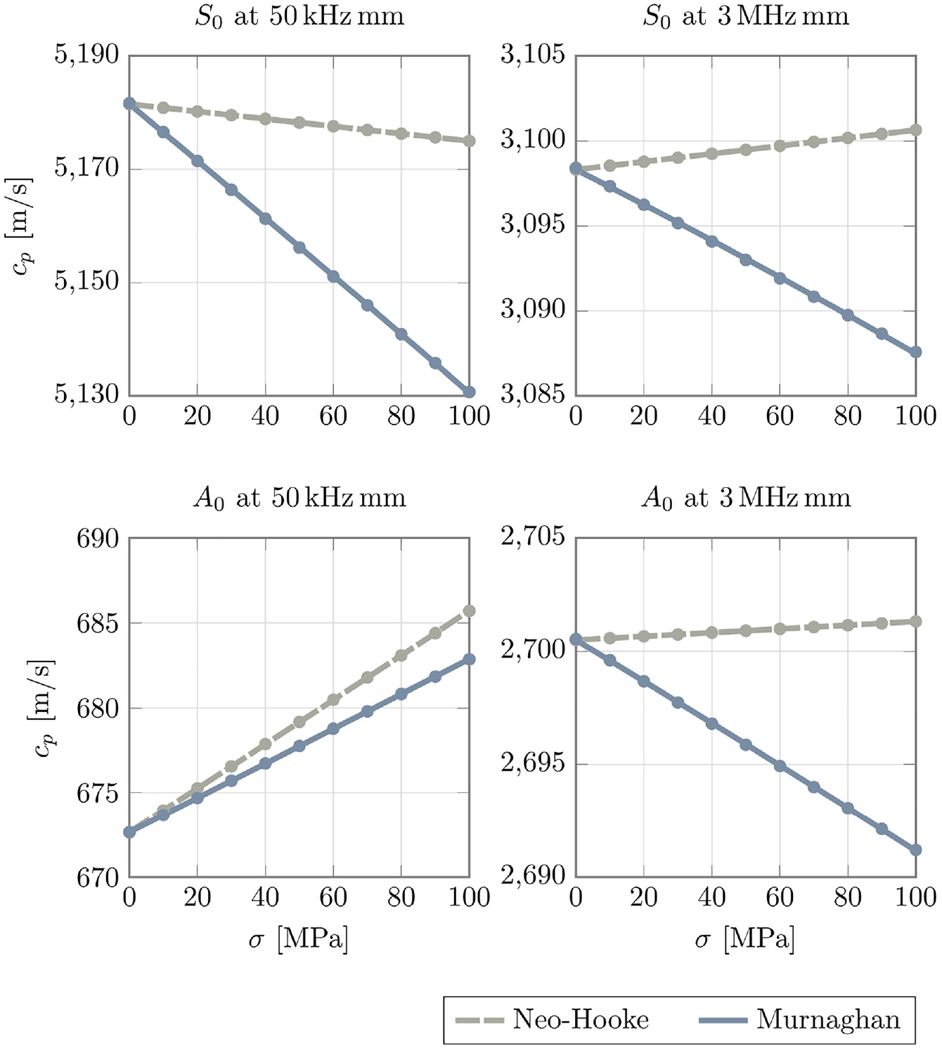
Phase velocities with increasing prestress at 50 kHz mm (left) and 3 MHz mm (right) for the Neo-Hooke and the Murnaghan material model. Upper row:
On the basis of these numerical results, it is not possible to assess which constitutive material model best reflects the physical phenomenon of acoustoelasticity. Therefore, a comparison with experimental results is made in the following.
Comparison with experimental results
In this section, the numerically obtained results are finally compared with the experimental data presented above. The comparison follows the same scheme as done before for the numerical and experimental data, respectively. First, the phase velocity difference is observed for certain load levels over the whole frequency range covered during the experiments. This is followed by the analysis of the correlation between the prestress level and the phase velocity difference.
Phase velocity
Figure 10 holds, on the one hand, the numerical results based on both the Neo-Hooke and Murnaghan material model as well as the experimental data for the
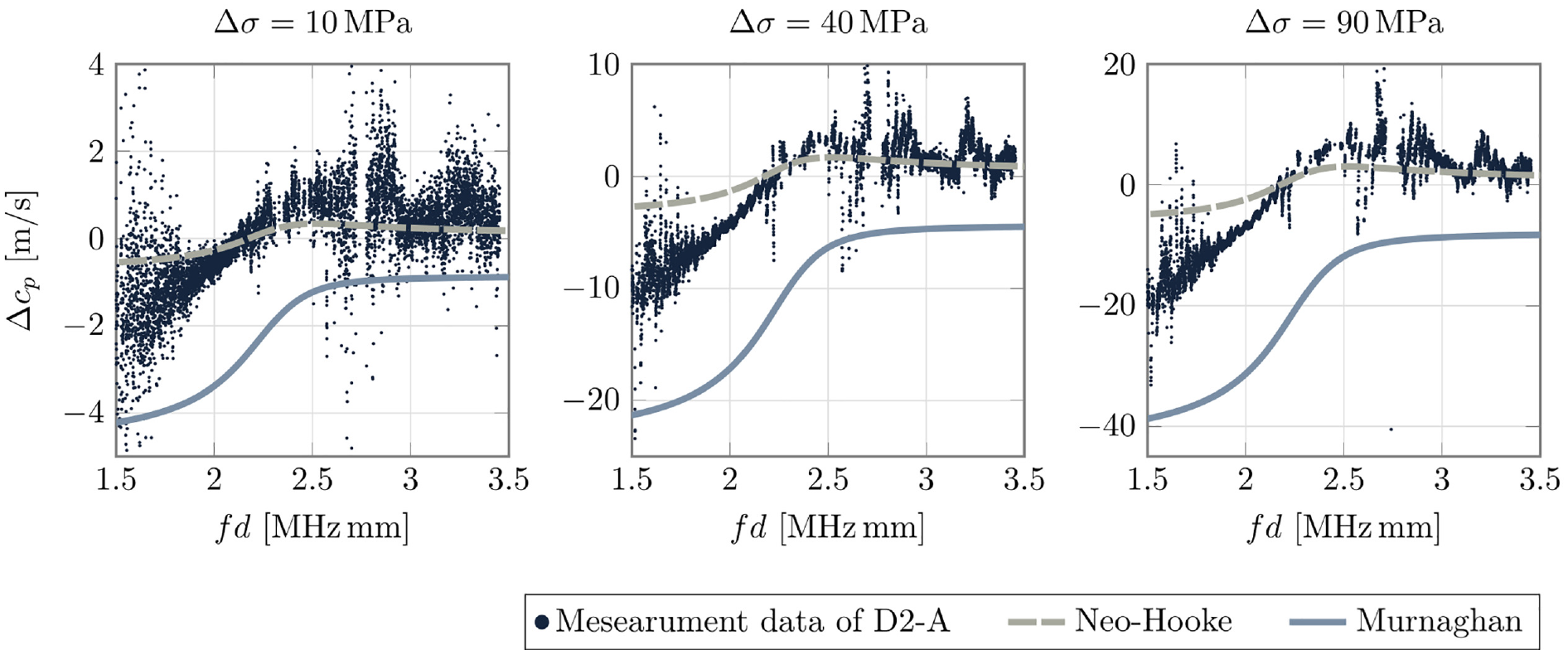
Comparison of the phase velocity difference
Figure 10 reveals that the numerical simulations based on the Neo-Hooke material model clearly reproduce the course of the measured data better than those based on the Murnaghan model. This applies here for all load steps considered. It is particularly noticeable in this comparison that both the measurement data and the Neo-Hooke data show a sign change in the phase velocity difference from negative to positive. This is not the case for the Murnaghan data. A more precise comparison shows that the Neo-Hooke data also shows a difference from the measured data. However, the comparison of the data curves is in a very good range.
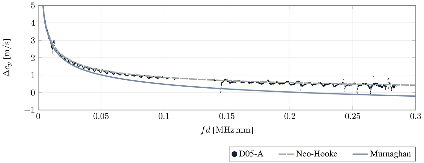
Figure 11 shows the experimental data from specimen D05-A and the numerical data for the
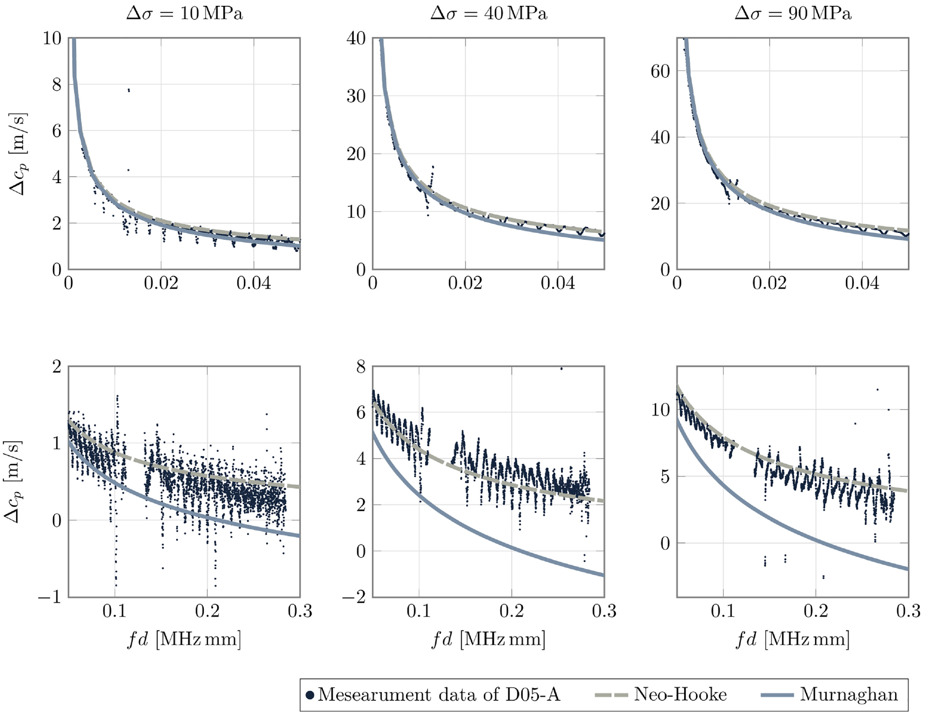
Comparison of the phase velocity difference
In Figure 12, the comparison of the
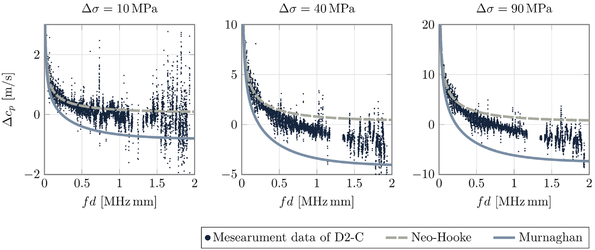
Comparison of the phase velocity difference
Following this, it is concluded that for the
Stress
As already discussed in the context of the experimental data, the comparison is extended to the linear regression of the phase velocity as a function of the prestress state difference. Due to the quality of the measurement data and the derived phase velocity differences, this comparison is limited to the
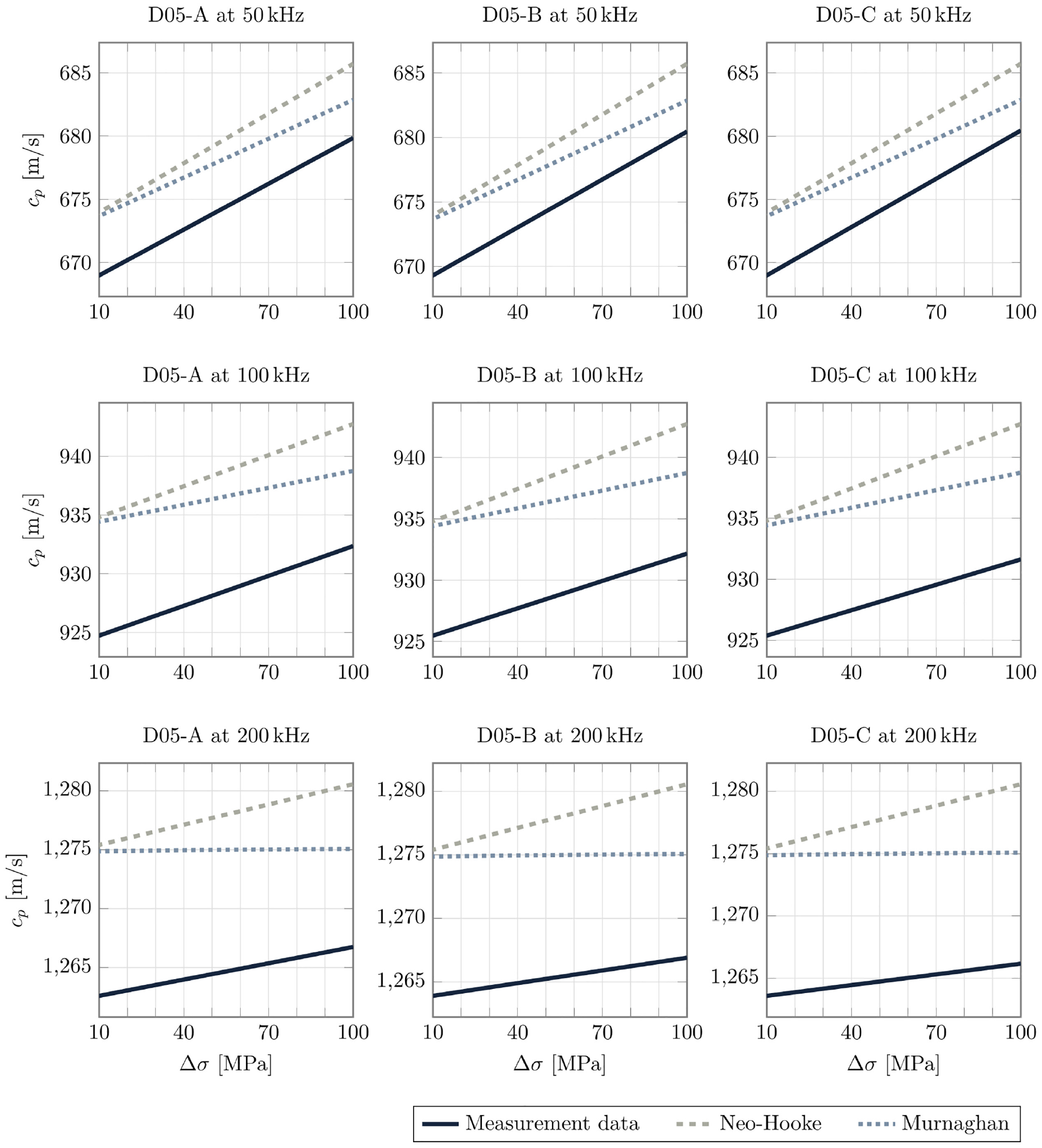
Comparison of the linear regression based on the measurement data for the three specimens D05-A, D05-B, and D05-C with results derived from numerical simulation taking into account the Neo-Hooke and Murnaghan material model.
The comparison meets the expectations. The slopes of the numerical data based on the Neo-Hooke material model fit very well with those from the experimental data. For the Murnaghan material model, on the other hand, the slope differs significantly. However, due to a variation in the material properties between the numerical simulation and the specimens, the initial phase velocity is not the same.
To depict the conclusion of this work in a more comprehensive way, the mean phase velocity difference for a load step of 10 MPa is computed for each frequency within the range of up to 0.3 MHz mm from the linear regression. Since the obtained value comprises the information of all analyzed load steps, it can be interpreted as the phase velocity difference due to a unity uniaxial load step of 10 MPa. The results are summarized in Figure 14 and reveal that the Neo-Hooke material model is very suitable for the representation of the acoustoelastic effect in a frequency range of up to 0.3 MHz mm.
Comparison of the computed unity uniaxial load step of 10 MPa for both the Neo-Hooke and Murnaghan material model with the experimental data of the specimen D05-A.
Summary and conclusion
This work deals with both numerical and experimental methods for investigations of acoustoelastic problems. The methods are exemplarily applied to GUWs in prestressed aluminum waveguides. The results are presented and discussed and serve to verify the numerical model.
First, the continuum mechanical fundamentals of wave propagation in prestressed structures are discussed. The material behavior is assumed to be hyperelastic, and the Murnaghan material law, which is often applied to acoustoelastic problems, and the Neo-Hooke material model, which is broadly used and less complicated to handle, are proposed for the constitutive description.
The aim of the experimental investigations is to determine the phase velocities of the fundamental wave modes
The numerical analysis is carried out using the finite element method. First, the prestress in the specimen is calculated in a nonlinear computation. The associated phase velocities of propagating waves are determined as a result of an eigenvalue analysis on a small unit cell of the specimen. The resulting dispersion diagram is valid for the previously determined prestress. This procedure is computationally very effective and has the advantage that it can be carried out with standard finite element programs. Therefore, it is an appropriate and useful alternative to the SAFE method, which is frequently used for this purpose.
A number of results first show that the experimental and numerical methods proposed in this work provide plausible results. It is also demonstrated that the numerical and experimental results are in very good agreement with the experimental data. Even though individual experimental observations are not exactly reproduced, the comparison shows, on the whole, that the Neo-Hooke material model approximates the experimental results better than the Murnaghan model. This result is significant because the Neo-Hooke model requires fewer material parameters than the Murnaghan model, is therefore easier to handle, and is available in most finite element program systems.
Future work will deal with layered and complex material systems, for example, fiber metal laminates, more complex prestressing states as well as residual stresses.
Footnotes
Acknowledgements
The authors expressly acknowledge the financial support for the research work on this article within the Research Unit 3022 Ultrasonic Monitoring of Fibre Metal Laminates Using Integrated Sensors by the German Research Foundation (Deutsche Forschungsgemeinschaft (DFG)).
Declaration of conflicting interests
The author(s) declared no potential conflicts of interest with respect to the research, authorship, and/or publication of this article.
Funding
The author(s) disclosed receipt of the following financial support for the research, authorship, and/or publication of this article: The work was funded within the Research Unit 3022 Ultrasonic Monitoring of Fibre Metal Laminates Using Integrated Sensors by the German Research Foundation (Deutsche Forschungsgemeinschaft (DFG)).