Sage Journals: Discover world-class research

Abstract

Fibrous plaster (FP) ceilings were commonly used in historic buildings throughout the UK during the 19th and 20th centuries. These ceilings are typically supported by hanger elements called wads, which are made of woven jute fabric embedded in plaster of Paris (POP). Recent collapses of several FP ceilings have raised concerns on our ability to detect and localise damage in wads before they fail. To address this issue, we propose a novel acoustic emission (AE)-based system for non-invasive failure detection and localisation. In particular, we develop a three-stage approach that employs 1D convolutional neural networks (1D-CNNs) to analyse AE waveform data produced by pencil-lead break sources for 2D AE source localisation. The approach involves training and fine-tuning four 1D-CNN models with varying architectures, followed by an ensemble learning method to improve localisation accuracy. AE waveform data is recorded using several sensor cluster geometries, with four sensors arranged in a square cluster. Two AE sensor spacing configurations (50 mm and 30 mm) are investigated. The approach also considers the scenario when only three waveforms are available. Experimental results indicate that for input data containing four waveforms, more than 90% of the source location estimations have an error less than 20 mm regardless of the spacing. When only three waveforms are available, 88% of the source location estimations have an error less than 20 mm. The results show that the proposed approach accurately localises source without prior knowledge of wave propagation velocities in the structure. The results are benchmarked with the beamforming method. The proposed approach provides computational simplicity, improved positioning accuracy and fewer constraints related to sensor locations. This approach may facilitate non-invasive damage detection and localisation in the wads of historic FP ceilings by conducting AE measurements on the underside of ceilings. This approach can also be applied to other anisotropic plate-like structures.

Keywords

Acoustic emission natural fabric-reinforced composite material plate-like structure acoustic source localisation square-shaped sensor clusters convolutional neural network fine-tuning ensemble learning

Introduction

Fibrous plaster (FP) is a natural fabric-reinforced composite material that comprises plaster of Paris (POP) as the matrix material and loosely woven jute fabric layers as the reinforcement material. This material has been widely used for suspended decorative ceilings in many historic buildings throughout the United Kingdom since the late 19th century.¹ Figure 1 presents the typical structure of a historic FP-suspended ceiling that consists of two critical structural components: the ceiling panel and the hangers (‘wads’), both of which are made of FP. The ceiling panel is in the form of a laminated composite material, and the cross-section of a historic FP ceiling panel is shown in Figure 2. Large historic FP ceiling panels also feature timber elements that are embedded in the POP matrix. The ceiling panel is suspended from a timber/metal framework located in the ceiling void, which is the space between the structural floor and the ceiling panel, via wads.²

Figure 1.

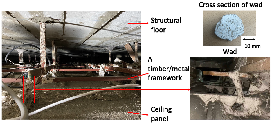
Typical structure of a historic FP-suspended ceiling.

Figure 2.

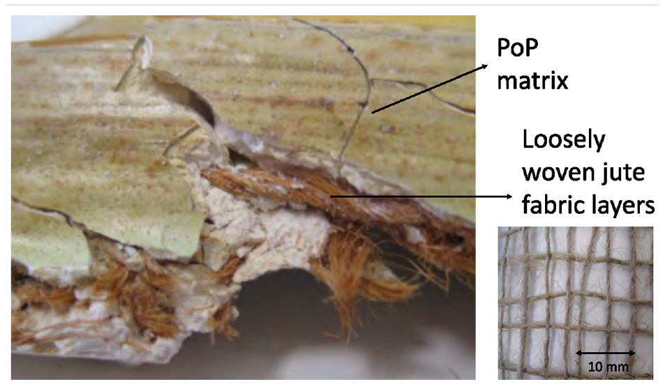
Cross-section of a historic FP ceiling panel.

Due to limited knowledge of the mechanical properties of FP and the structural behaviour of FP-suspended ceilings, inspections are subjective and error-prone. The current guidance for FP ceiling inspections relies on periodic visual and tactile assessments performed by experienced inspectors. This method necessitates the creation of access hatches on the ceiling, which can be costly.³ Recent collapses of several historic FP ceilings in London highlighted the need for more accurate and objective monitoring approaches. Since FP ceiling collapses are often ascribed to failures in the wad elements which are inaccessible from the underside of the ceiling, the monitoring needs to be done remotely. Acoustic emission (AE) techniques have a proven track record in conducting remote damage localisation in anisotropic plate-like structures.^4,5 These techniques facilitate the identification of failure sources through non-destructive means, ensuring that the implementation process does not impose any detrimental effects on the integrity of the original building structures. This article examines a novel application of this approach to historic FP ceilings. The current paper does not differentiate between different failure types but focuses solely on localising the wad where a failure mechanism is generating AE events.

A generic block diagram illustrating an AE-based Structural Health Monitoring (SHM) system for damage source localisation in anisotropic plate-like structures is presented in Figure 3. AE signals produced by the rapid release of energy from microscopic failures can be acquired in situ. The recorded signals are used to estimate the location of the failure source using an array of sensors placed at the surface of the structure, with varying distances to the failure source, which can detect the respective AE waveform at different times.^6,7 The subsequent damage assessment and maintenance are also depicted, but are outside the scope this article and will not be explained in detail. With regards to localisation on homogeneous materials, the measured difference in the time-of-arrival (TOA) of AE signals can be converted directly into the distance between the sensor and the damage source due to the constant AE wave propagation velocity.⁸ However, source localisation for historic FP ceiling panels remains a key challenge in practical applications. The TOA-based conventional methods are not suitable for the historic FP-suspended ceilings since the AE wave propagation is strongly influenced by anisotropy.⁷ The direction- and location-dependent wave velocities are infeasible to measure due to the size and geometric complexity and variation of the composite structure.⁹ Therefore, there is a need for a method that can be used for source localisation in historic FP ceiling panels that does not utilise the wave propagation properties of the structure.

Figure 3.

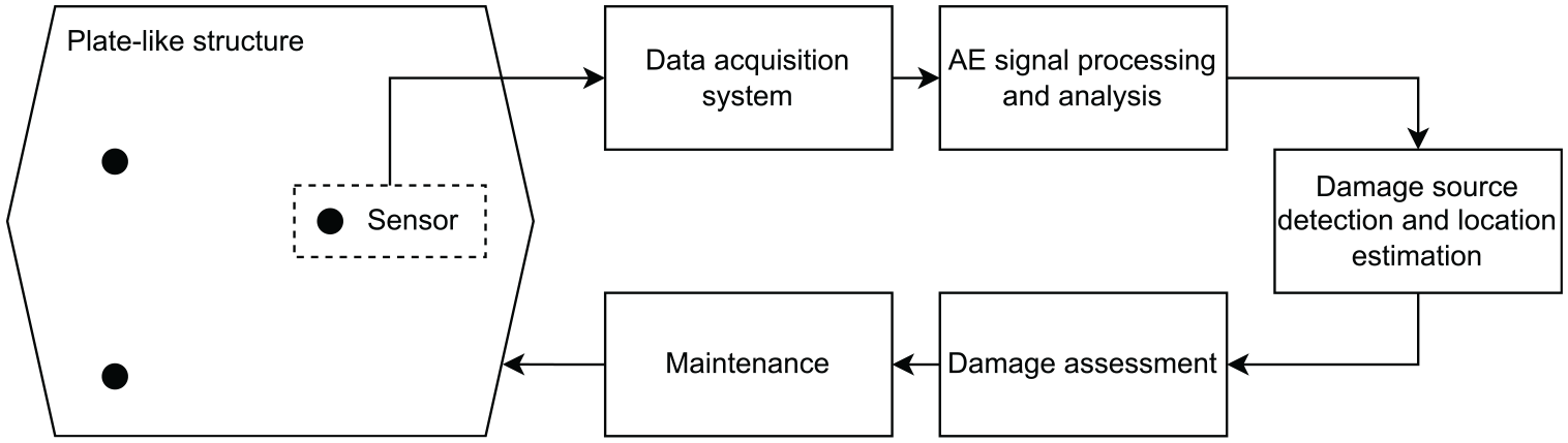
Block diagram of an AE-based SHM system for damage source localisation of plate-like structures.

Many methods have been proposed to improve the accuracy of the source localisation in anisotropic structures, as summarised in a recent review.⁸ The time difference of arrival (TDOA) methods are popular in localising AE sources without pre-measuring wave velocities.^10,11 One specific technique in source localisation of plate-like structures is called the sensor cluster technique. This technique is mostly used by the beamforming method proposed by Kundu et al.¹² This method assumes that the velocities of the waves propagating from the source to the sensors are all the same due to the nature of the sensor cluster. Therefore, it does not require the wave propagation properties of anisotropic materials. The beamforming theory estimates wave incidence angles based on the geometry of sensor cluster placement. As shown in Figure 4, a classic L-shaped sensor cluster consisting of three receiving sensors (S1, S2 and S3) is placed on a plate-like structure. This is based on the understanding that three sensors represent the minimum number required for achieving two-dimensional AE event source localisation. The method assumes that the wave has a straight propagation path from the AE source to the sensor cluster. It can be assumed that the wave velocity of the straight path connecting the AE source to each sensor is approximately the same since the sensor spacing $d$ is much smaller than the distance between the AE source and the nearest sensor $D$ , resulting in similar signals with a slight time offset. The time offset can be used to determine the TDOA, which is the time it takes for the wavefront propagating from the source to reach sensors S2 and S3 after reaching S1. The results, denoted as $δ t_{12}$ and $δ t_{13}$ , can be derived as $d \cos (θ_{1}) / c (θ)$ and $d \sin (θ_{1}) / c (θ)$ , respectively, where $c (θ)$ represents the wave velocity in the $θ$ direction. The wave incidence angle $θ$ can be obtained without requiring any information on the wave propagation velocity. This angle can be expressed as $\tan^{- 1} (δ t_{13} / δ t_{12})$ . In many studies, multiple sensor clusters are used to estimate AE source locations in anisotropic plate-like structures based on beamforming theory, owing to its computational simplicity and high accuracy.^13–19 However, the beamforming method has some disadvantages. The accuracy of the source localisation largely depends on the accuracy of the TDOA measured from the AE waveform recorded by the sensor cluster. This TDOA is used to estimate the wave incidence angle at a specific location on the plate-like structure.²⁰ This wave incidence angle may deviate notably from the actual wave incidence angle, leading to significant errors in the source location estimation.

Figure 4.

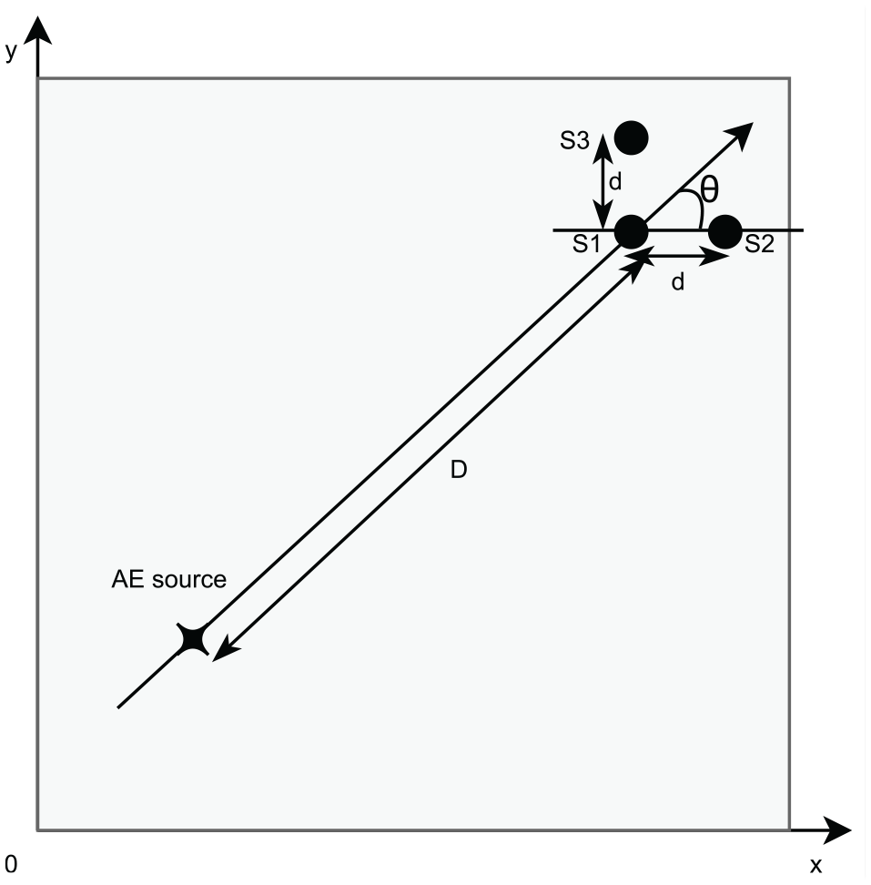
Basic L-shaped sensor cluster for TDOA-based beamforming technique.

Several approaches have been developed to enhance the accuracy of source localisation. Nakatani et al.²⁰ proposed a method for localising sources on anisotropic flat plates using two L-shaped sensor clusters. Only the initial part of the AE waveform signal is extracted to improve the accuracy of the TDOA measurement. This method has high accuracy in estimating source locations, and the direction error is limited to within +10°. However, the approach relies heavily on the accurate identification of first arrival waves, which is either done manually or by using arrival time detection algorithms such as the Akaike information criterion method.²¹ Wavefront shape-based methods estimate source location using techniques such as time-delay estimation and direction-of-arrival estimation.^14,22,23 This method assumes that the AE wavefront propagates in a specific way, such as a spherical wave or a cylindrical wave. Sen et al.¹⁴ used a wavefront shape-based approach by applying a square sensor cluster consisting of four L-shaped sensor clusters to improve the accuracy of source localisation. However, the signal processing required to estimate the direction of arrival can be computationally intensive, resulting in longer processing times and greater computing resource requirements. Furthermore, in practical environments, the wavefront may not obey the assumption that the AE wavefront propagates as a spherical or cylindrical wave, which leads to errors in the estimation of the source location. Neural network techniques have also been employed to improve the accuracy of source localisation using sensor clusters.^24–26 Fu et al.²⁷ applied the square-shaped sensor cluster for the source localisation on the plate-like anisotropic structure by establishing a neural network model. The model takes the measured TDOA as input data and the coordinates of damage sources as labels. The results report high accuracy. However, TDOA measurements based on the obtained group velocity distribution in composite materials are not suitable for practical situations. The velocities can be measured experimentally for specific test objects but are generally not applicable to other structures. Any method that requires knowledge of the wave propagation properties in a plate-like anisotropic structure may, therefore, be of limited practical use.

The sensor cluster technique could be an appealing option for source localisation in historic FP-suspended ceilings. However, accurately and automatically extracting the information present in the AE waveform recorded by the sensor cluster can be challenging and requires novel methods. It has been reported that one-dimensional convolutional neural networks (1D-CNNs) can automatically extract features from AE waveform data and can be directly trained using such one-dimensional time-series signals.²⁸ Therefore, one possible approach to extract information from the AE waveform is to use 1D-CNNs.

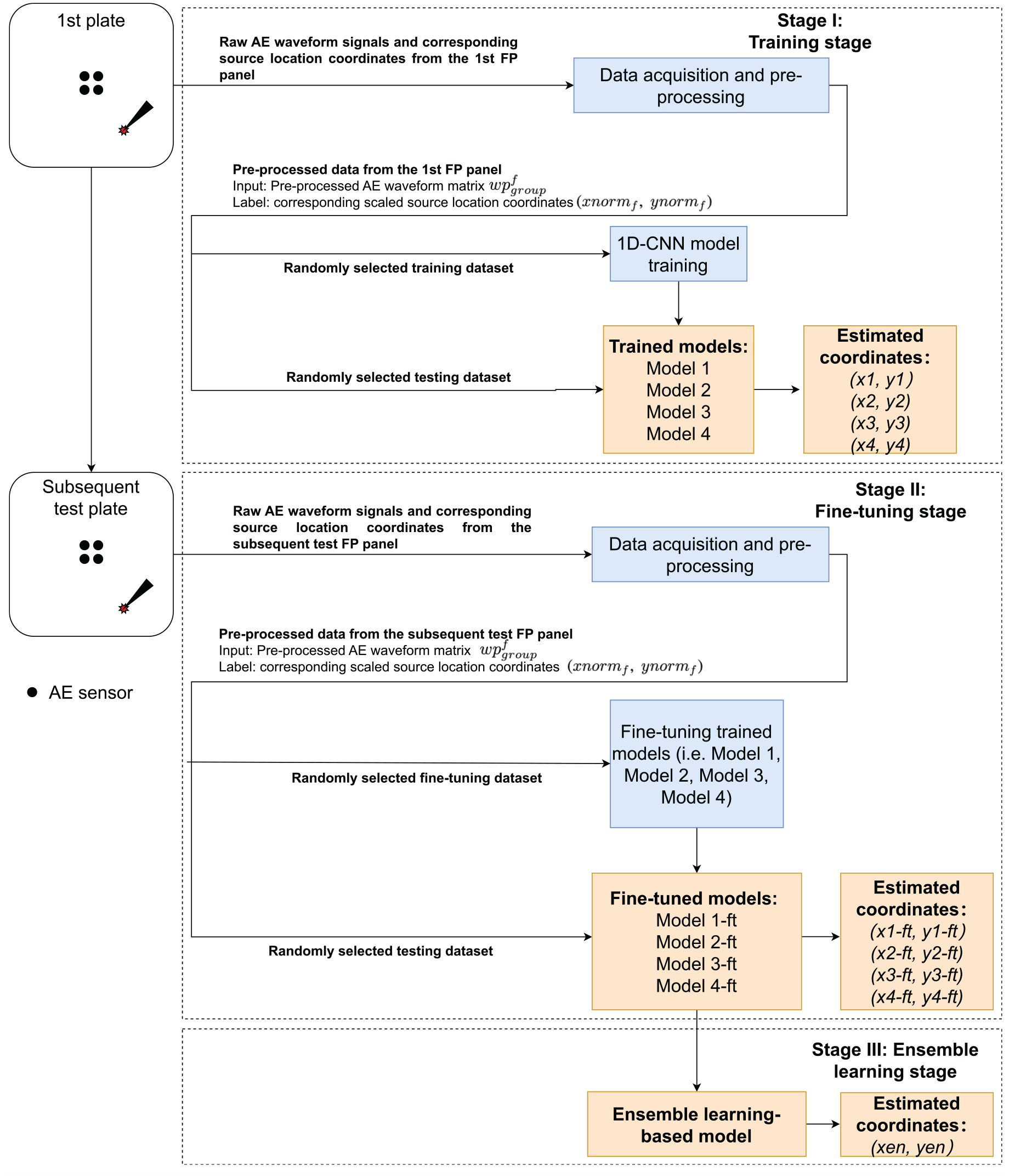
This study presents a novel approach to AE source localisation, using 1D-CNNs to accurately estimate the locations of AE sources on historic FP ceiling panels. To achieve this, a square-shaped sensor cluster is used to record AE waveform data, and the 1D-CNN is used to estimate the source location directly using the AE waveform data without requiring any prior knowledge of wave propagation properties or TDOA measurements. A three-stage approach is proposed for achieving the objective. In stage I, a large amount of data is used to train four 1D-CNN models with different dropout layer implementations. In stage II, the trained models are fine-tuned using a smaller dataset from a new test object, in this case, a historic FP ceiling panel, to make the models adaptable to new test objects and able to perform AE source localisation using a limited amount of data and a short duration of fine-tuning. This historic FP ceiling panel is considered a new test object in practice, and the fine-tuning process is carried out for each new test object. In stage III, an ensemble learning approach is used to combine the localisation results provided by the fine-tuned models, which can significantly improve the localisation accuracy. 1D-CNN models take AE waveform data as input, and the corresponding AE source coordinates as labels. The results are benchmarked using the established TDOA-based beamforming method, which also uses sensor clusters.

The article is organised as follows: It commences with a brief introduction that presents an overview of the methodologies employed, including the data acquisition system and signal processing. This is followed by a detailed description of the designed CNN architectures and the different implementation details, along with an overview of the three-stage approach for establishing 1D-CNN models. The subsequent section describes the experimental setup utilised for AE waveform data collection, followed by the results obtained for AE source localisation in historic FP ceiling panels using the developed 1D-CNN-based method. Finally, a comprehensive assessment of the performance of the developed 1D-CNN method is presented.

Methodology

A block diagram illustrating the steps involved in developing the AE source localisation method, including data acquisition, signal processing and the implementation of a 1D-CNN architecture, is shown in Figure 5.

Figure 5.

Block diagram of the steps involved in developing the AE source localisation method.

Data acquisition system and test configuration

The system is designed with four AE sensors denoted as S1, S2, S3, S4 arranged in a square configuration, mounted at the centre of a square-shaped monitoring area of a plate-like test object. Pencil-lead break sources are generated at pre-determined coordinates. Each sensor receives a single raw AE waveform generated by the pencil-lead break source. For a given pencil-lead break, each of the four sensors records a voltage waveform containing 4096 waveform data points at a data collection frequency of 2 million samples per second, as shown in Figure 6.

Figure 6.

Raw single AE waveform signals generated by one pencil-lead break source recorded by sensors S1, S2, S3, S4 of the square-shaped sensor cluster of default configuration.

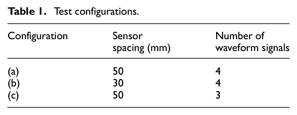
Three distinct configurations for testing are devised, as shown in Table 1. The sensor layout of configurations (a) and (b) are shown in Figure 7. Configuration (a) is the default configuration. Configuration (b) investigates the influence of sensor spacing on the accuracy of the proposed method. The selection of specific configurations involving the utilisation of a sensor cluster with 30 and 50 mm spacing of AE sensors is grounded in the prior work referenced within the paper,¹² which examined sensor spacings of 15, 30 and 50 mm. As shown in Figure 4, the study concluded that reducing the ratio of sensor cluster spacing d to the distance D between the acoustic source and the sensor cluster contributes to improved localisation accuracy. This enhancement can be attributed to a fundamental assumption of the localisation technique, where the lines connecting the acoustic source point to distinct sensors within the cluster exhibit a nearly parallel alignment, a condition met when d/D ratios are low. However, in this study, due to the sensor dimensions (with a diameter of 19 mm), it is impossible to achieve a sensor spacing of 15 mm. Consequently, the 30- and 50-mm configurations were selected. The input data for configuration (c) is generated by randomly dropping one waveform collected by one sensor for each pencil-lead break source using the dataset from the default configuration (a) using the same sensor layout. This configuration considers the scenario when one waveform is not recorded, which can happen due to sensor malfunction.

Table 1.

Test configurations.

Configuration	Sensor spacing (mm)	Number of waveform signals
(a)	50	4
(b)	30	4
(c)	50	3

Figure 7.

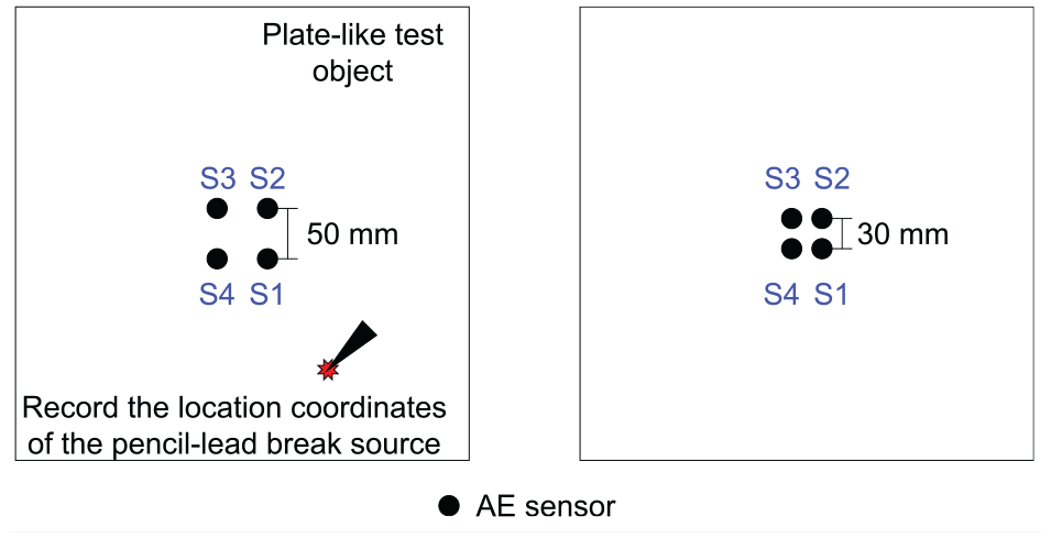
Square-shaped AE sensor clusters with 50 mm for configuration (a) (left) and 30 mm for configuration (b) (right) sensor spacing mounted on a plate-like test object.

AE signal processing

All raw AE waveform data generated by the same pencil-lead break source is synchronised and then organised into a 4 × 4096 matrix. Each matrix is normalised using L2 normalisation, also known as Euclidean normalisation. This ensures that the norm of the normalised vector or matrix is equal to 1, and the matrix is more comparable to other matrices with different scales or magnitudes.

Only the initial portion of each waveform up to the peak amplitude (PA) − is selected for learning (see Figure 8). This initial portion of the signal, during its rise time (RT)’, − records the Lamb wave. Lamb wave is a type of ultrasonic guided wave that propagates through the plate-like structures and is not significantly affected by reflections from other sensors or the edge of the plate.²⁰ This truncation results in waveform lengths less than 4096. The waveforms are then zero-padded back to a length of 4096 to achieve consistency between input signals.

Figure 8.

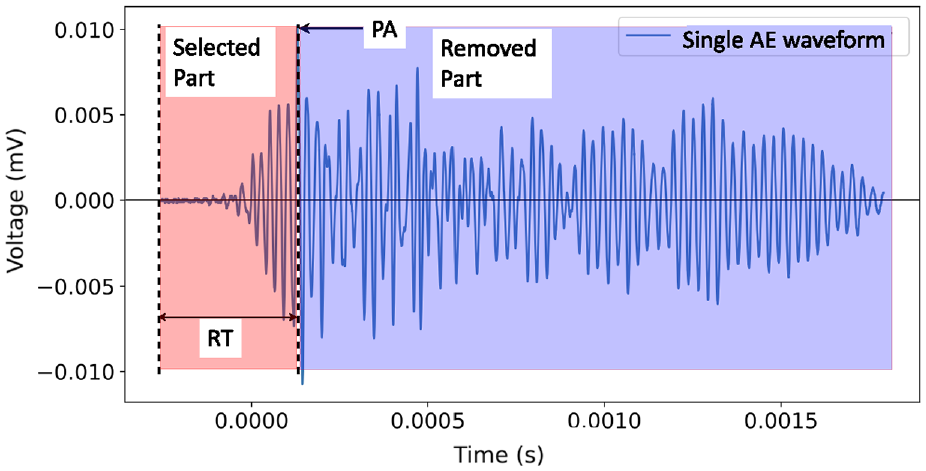
A typical AE waveform with a description of peak amplitude (PA) and rise time (RT).

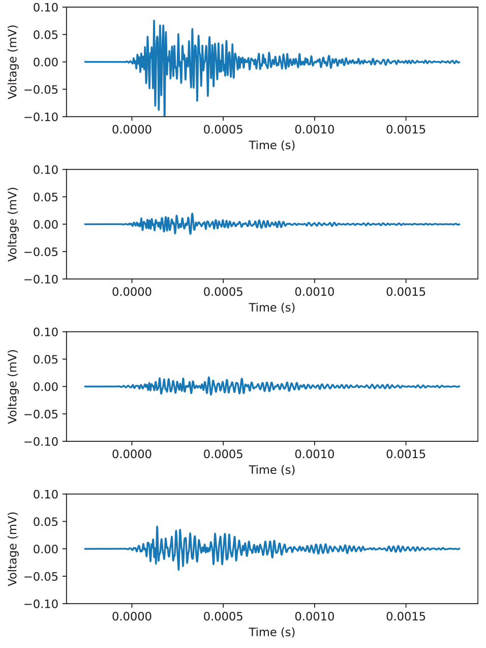
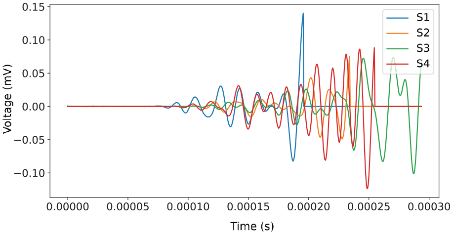
Figure 9 displays an example of a waveform matrix composed of four pre-processed AE waveform signals following a pencil-lead break event. The matrix featuring the pre-processed AE waveform signals is denoted as $w p_{group}^{f}$ , where $f$ is the AE source index. The coordinates of the corresponding pencil-lead break sources are scaled to a range between 0 and 1 and used as the output label for the 1D-CNN model learning. The normalised coordinate of the pencil-lead break source is denoted as $(x nor m_{f}, y nor m_{f})$ . $w p_{group}^{f}$ and $(x nor m_{f}, y nor m_{f})$ are subsequently used as input and label for the subsequent 1D-CNN models, respectively.

Figure 9.

Pre-processed AE waveform signals generated by one pencil-lead break source recorded by sensor S1, S2, S3, S4 of the square-shaped sensor cluster of default configuration.

CNN architecture and implementation details

CNN architecture

The CNN architecture used in this study is presented in Figure 10 with implementation details listed in Table 2. The model consists of four one-dimensional convolutional layers, each followed by a max pooling layer, and two fully connected layers. The convolutional layers have a kernel size of 5 and a stride of 1. The first, second, third and fourth convolutional layers (1DCONV1-1DCONV4) have output channel sizes of 32, 64, 128 and 256, respectively. Each max pooling layer (MP1 to MP4) has a kernel size of 2 and a stride of 2. The first fully connected layer (FC1) uses ReLU activation functions, while the second fully connected layer (FC2) uses Sigmoid activation functions since the target output values (i.e. normlised coordinates X and Y) are in the range of 0–1. The optimiser used is Adaptive Moment Estimation (ADAM), with an initial learning rate of 0.00075 and a cosine annealing scheduler, while the loss measure used is the Mean Squared Error (MSE).

Figure 10.

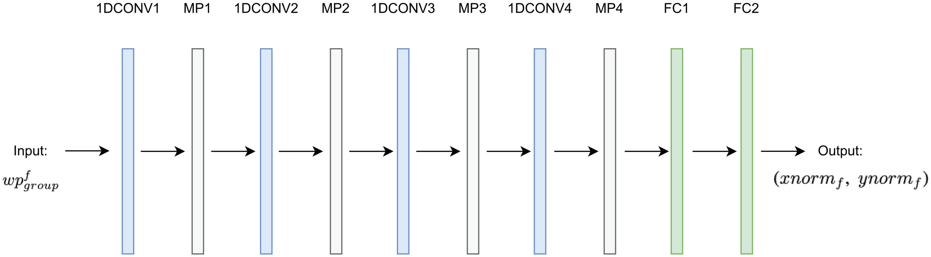
Adopted 1D CNN architecture.

Table 2.

Designed CNN architecture.

Layer type	Input size	Output size	Filter height	Stride
1DCONV1	4 × 4096	32 × 4092	5	1
MP1	32 × 4092	32 × 2046	2	2
DCONV2	32 × 2046	64 × 2042	5	1
MP2	64 × 2042	64 × 1021	2	2
DCONV3	64 × 1021	128 × 1017	5	1
MP3	128 × 1017	128 × 508	2	2
DCONV4	128 × 508	256 × 504	5	1
MP4	256 × 504	256 × 252	2	2
FC1	256 × 252	1000	–
FC2	1000	2	–

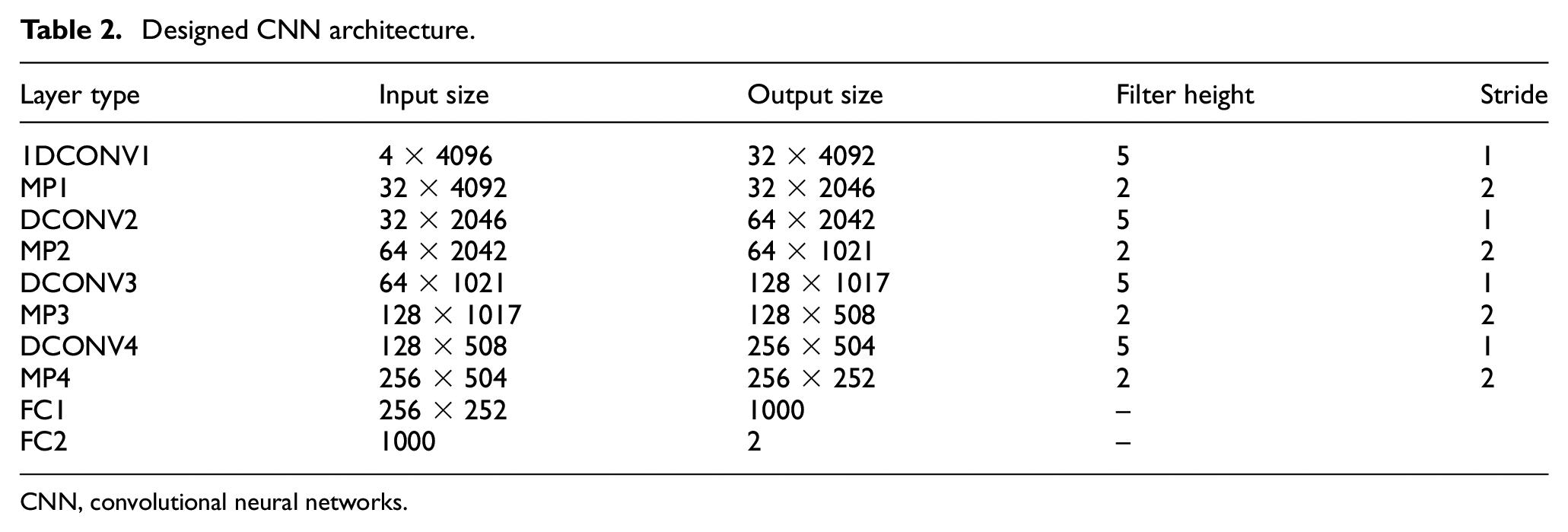
CNN, convolutional neural networks.

Dropout layer implementation

Dropout is a regularisation technique to prevent over-fitting in neural networks. It randomly drops out − by setting the corresponding weights to 0 − neurons in the network during training with a probability of p. This exercise forces the network to learn more robust features and reduces its dependence on specific input features.

Different dropout layer implementations can introduce diversity in CNN models during ensemble learning. Ensemble learning involves aggregating predictions from different models. By combining predictions from 1D-CNN models with different dropout layer implementations, the overall predictive performance can be improved by reducing generalisation errors. It can also help to identify the strengths and weaknesses of each model and combine them in a way that maximises their benefits and minimises their drawbacks.

For the purpose of subsequent ensemble learning, four CNN models were trained using different dropout layer implementations, outlined in Table 3.

Table 3.

Dropout layer implementations for different independent 1D-CNN models.

CNN model	Layer with the dropout layer applied	Dropout probability p
Model 1	FC2	0.3
Model 2	FC1	0.3
Model 3	FC1	0.5
Model 4	FC1	0.1

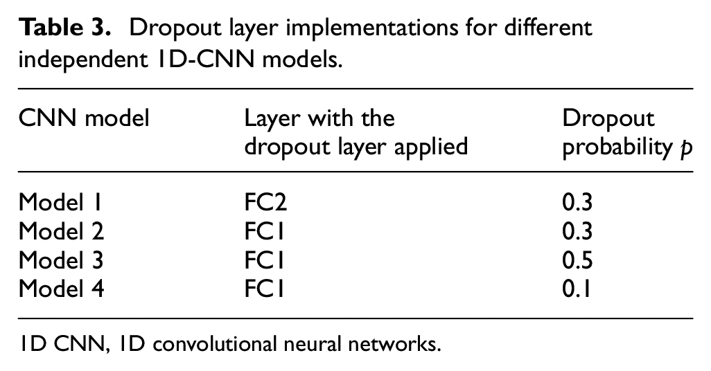
1D CNN, 1D convolutional neural networks.

D-CNN models

To develop 1D-CNN models for AE source localisation that can be applied to various historic FP ceiling panels, this study utilises two plate-like test objects, both of which are historic FP ceiling panels from the same site. The first FP panel is employed in stage I, where a large amount of data is recorded and used to train 1D-CNN models. The subsequent test FP panel is utilised in Stages II and III, where a small amount of data is collected to fine-tune the models trained in stage I and perform ensemble learning, respectively.

The use of two test objects allows for the assessment of the models’ adaptability to new testing scenarios and the evaluation of the effectiveness of the proposed three-stage approach. The subsequent test object simulates a new area for monitoring, obtained from the same site as the first panel. The fine-tuned models and ensemble learning analysis are evaluated based on their ability to accurately localise AE sources on the subsequent test object, using a limited amount of data. This evaluation holds great practical significance for non-destructive testing applications.

For each site-specific application, stage I only needs to be conducted once on a randomly selected area of the monitored FP ceiling site. Stages II and III are required to be conducted for any new area of the site that needs monitoring, where a small dataset must be acquired for fine-tuning the model trained in the first stage.

Stage I: Training stage

During the training stage, the 1D-CNN models take $w p^{f} group$ and $(xnormf, y_{normf})$ from the first FP panel as input and label, respectively. Four 1D-CNN models, Model 1, Model 2, Model 3, Model 4, with the mentioned architecture and dropout layer implementations, were trained independently. The estimated coordinates given by Model 1, Model 2, Model 3, Model 4 are denoted as (x1, y1), (x2, y2), (x3, y3), (x4, y4), respectively. The estimation error is calculated by finding the difference between the recorded and the estimated coordinates, which can be denoted as $Er r_{pre}$ . The total number of epochs during training is 150. The batch size for training is 1.

Stage II: Fine-tuning

In the fine-tuning stage, the 1D-CNN models trained with weights from stage I are adopted for additional training with a small dataset containing $w p^{f} group$ and $(x nor m_{f}, y_{nor m_{f}})$ from the subsequent test FP panel. The idea is to allow the trained models from the previous stage to learn task-specific features that are important for each new test object while still retaining the knowledge learned from the original dataset. The total number of epochs during training is 50, and the batch size is again 1. Using a smaller dataset and epoch number for fine-tuning the new object can help reduce the computational cost and time required for fine-tuning the model. However, it is important to ensure that the smaller dataset is representative of the new object and contains enough information for the model to learn meaningful features.

During this stage, the first two convolutional layers of the model are frozen, whereas the weights of other layers are updated to better capture the subsequent test panel data while training. The optimiser and loss functions remain unchanged. The estimated coordinates given by Model 1-ft, Model 2-ft, Model 3-ft, Model 4-ft are denoted as (x1-ft, y1-ft), (x2-ft, y2-ft), (x3-ft, y3-ft), (x4-ft, y4-ft), respectively. The performance of the fine-tuned models from this stage is evaluated by calculating the difference between the recorded and estimated coordinates using a new dataset from the same test object for the fine-tuning, represented as $Er r_{ft}$ .

Stage III: ensemble learning

As a final refinement, estimations of the source location provided by the four distinct fine-tuned CNN models are subsequently combined. This approach seeks to harness the collective insights of these models for enhanced accuracy. Specifically, the two most proximate predictions of coordinates are averaged, leading to the computation of the final estimated coordinates, denoted as (xen, yen). To gauge the accuracy of the ensemble learning’s final estimation, the disparity between the recorded coordinates and the estimated ones is computed, presenting itself as the quantified error $Er r_{el}$ .

Experiment

Test objects

Initially, AE data was collected from a POP (i.e. the matrix material of the FP) plate to train the aforementioned 1D-CNN models. This was done to ensure that the method could first be applied to simple homogeneous materials before moving on to complex anisotropic FP structures. 1D-CNN Model 1 and the default test configuration (a square-shaped sensor cluster with a sensor spacing distance of 50 mm) were employed. In this experiment, a total of 200 groups of data were collected from a POP plate-like test object, out of which 130 groups (65%) were used for training, 20 groups (10%) were used for validation during the training process for each epoch, and 50 (25%) groups were used for testing.

Two historic FP ceiling panels, sourced from the Great Stairs of the Institution of Civil Engineers (ICE) building (constructed in 1912), were then used for the data collection. These historical ceiling samples, originally intended for replacement in the ICE building, have been repurposed for controlled laboratory data collection. AE data produced by pencil-lead break sources, along with the corresponding source location coordinates, are collected to establish 1D-CNNs based on the three-stage approach. The dataset used for training stage from the first FP panel consisted of 252 groups of effective data. Out of these, 172 groups (68%) were randomly selected for training, 30 groups (12%) for validation and 50 groups ((20%)) for the test dataset. The validation data was used to monitor the model’s improvement at each epoch, while the testing data was used to evaluate the performance of the models after they were trained. The dataset used for fine-tuning stage consisted of 149 groups of effective data collected from the subsequent test FP panel, of which 79 groups (53%) were randomly selected for training, 20 groups ((13%)) for validation, and 50 groups ((34%)) were used for testing. The same dataset is used for training, validation and testing for all four models, both during the training stage and the fine-tuning stage.

Figure 11 provides a visual representation of the test objects, including their cross-sectional views. The POP plate has a thickness of 10 mm, while the historic FP panels have a thickness ranging from 8 mm to 20 mm, excluding the timber laths. The timber laths are embedded inside with a thickness of around 40 mm. The historic FP panels are acquired through random selections from the onsite location. Their approximate dimensions are comprehensively detailed in Table 4.

Figure 11.

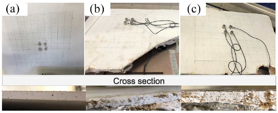
Plate-like test objects and cross sections of (a) POP plate, (b) the first historic FP panel, and (c) the subsequent test historic FP panel.

Table 4.

Test object description.

Test object	Material	Source	Area dimensions (m)	Purpose
POP Plate	POP	–	1 × 1	Validation with a simple homogeneous material
First FP Panel	historic FP	ICE Building, 1912	1 × 1	Stage I: Training
Second FP Panel	historic FP	ICE Building, 1912	0.8 × 1.2	Stages II and III: Fine-tuning and Ensemble learning

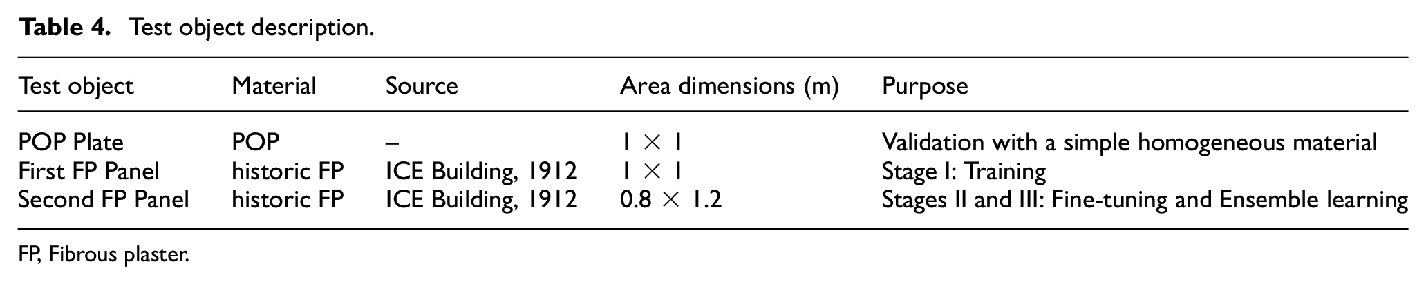
FP, Fibrous plaster.

Experimental setup

The experimental setup, as illustrated in Figure 12, consists of a Mistras system consisting of a 40 dB external amplifier, a four-channel PCI-2 AE data acquisition system, and four narrowband resonant AE sensors of model type R6a. The recorded signals are thresholded at 40 dB to eliminate noise. The ‘AEwin’ software is used to control the data acquisition process. A frequency band filter ranging from 35 to 100 kHz is used to filter the collected signal due to the low frequency of the AE signal generated by the plaster materials.

Figure 12.

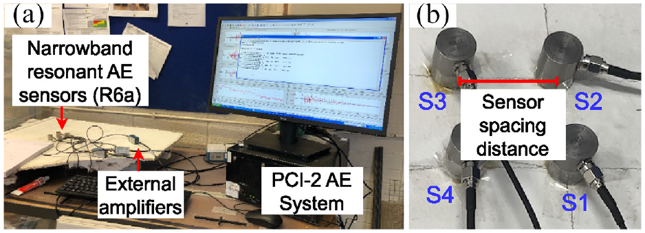
Experimental setup: (a) Measuring system and (b) square-shaped sensor cluster.

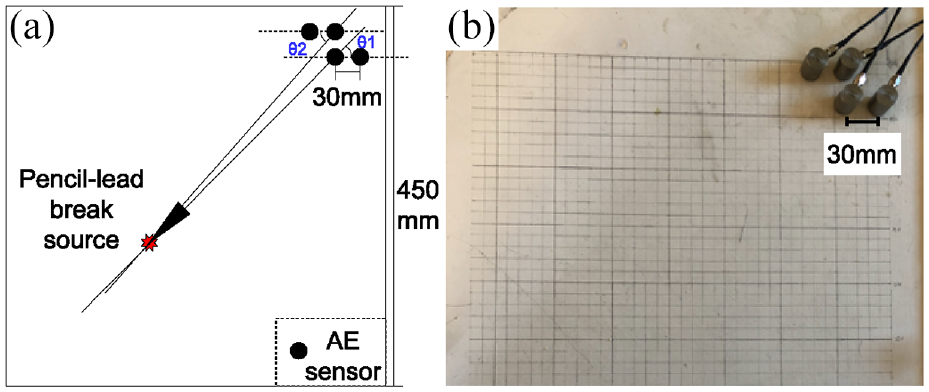
The square-shaped sensor cluster is mounted onto the surface of the test object, with a thin layer of grease applied in between to act as a coupling agent and improve the transfer of ultrasonic energy between the AE sensors and the surface of the test object. This allows for complete removal without causing lasting damage or alterations. For each test object, a flat 450 mm × 450 mm area was monitored. Since a threshold value of 40 dB is utilised, it means that if the AE signal released by an event exceeds this threshold value, the AE sensor can detect the event. If all four AE sensors in a sensor cluster detect the event, the AE cluster can localise the event source based on the received signal group. The attenuation curve indicates that the maximum detection distance for FP is approximately 1.5 m. Considering the geometry that the side length of a square is $\sqrt{2} / 2$ times the length of the diagonal, a maximum detection area of approximately 2 m-by-2 m is achievable. Pencil-lead break sources were randomly distributed across the entire monitoring area to ensure full coverage. Within the framework of the 50 mm sensor spacing configuration, AE sensors labelled 1–4 are strategically positioned at the following coordinates: (200, 200), (200, 250), (250, 250), and (250, 200). Correspondingly, in the context of the 30 mm sensor spacing configuration, AE sensors, each designated as 1–4, are positioned at the coordinates (210, 210), (210, 240), (240, 240) and (240, 210), respectively. In the process of generating pencil-lead break sources, random x and y coordinates are selected within the range spanning from 0 to 450. However, meticulous measures are undertaken to ensure that these sources are deliberately placed outside the confines of the sensor cluster. All measurements are in millimetres.

To benchmark the 1D-CNNs predictions, the TDOA-based beamforming method is also tested on a historic FP panel (first FP panel) using a well-established Z-shaped cluster,¹⁹ as shown in Figure 13. Two incidence angles, $θ_{1}$ and $θ_{2}$ , were identified using the two L-shaped sensor clusters contained in the Z-shaped sensor cluster. It should be noted that the paper that proposed this method¹⁹ used two Z-shaped sensor clusters positioned far apart for AE source localisation. However, in this study, a single Z-shaped sensor cluster was repeatedly used by placing it in two different locations to assess accuracy. Pencil-lead break sources were generated at the same positions for both scenarios. The initial part of the recorded signal was extracted manually, and the time shift was then determined using the cross-correlation method on the extracted waves as described in Nakatani et al.²⁰

Figure 13.

Z-shaped sensor cluster for TDOA-based beamforming method testing (a) schematic description, (b) experimental setup.

Accuracy of recorded source locations

Uncertainties

During the data collection process, the accuracy of the AE source location coordinates was affected by two factors. Firstly, a grid was manually drawn on the test object for assessing multiple AE sources, which may introduce an error of ±1 mm. Secondly, small variations in sensor positioning can occur (up to ±1 mm).

Accuracy thresholds for AE source localisation by 1D-CNNs

The 1D-CNNs used for AE source localisation have three accuracy thresholds: <20 mm for high accuracy, 20–100 mm for acceptable accuracy, and >100 mm for unacceptable accuracy. The 20 mm threshold was chosen as wads typically have diameters between 20 and 30 mm.

Results and discussion

Source localisation results on POP plate using 1D-CNN

The results of the AE source localisation are presented in Figure 14. The lines connect the predicted source location to the ground truth values, with different colours indicating the level of accuracy. Blue, green and red lines represent high, acceptable and unacceptable accuracies, respectively. The percentage distribution of accuracy levels is summarised in Table 5. Out of the 50 test data groups, 96% had high to acceptable accuracy, indicating the good performance of the 1D-CNN method for simple homogeneous materials.

Figure 14.

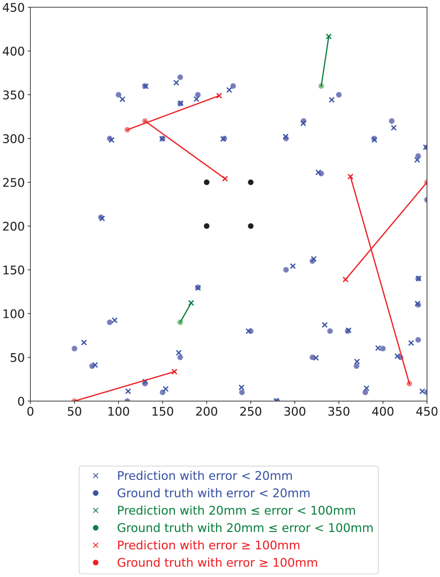
Exemplar AE source localisation results for the POP plate using 1D-CNN model Model 1, axis labels in units of mm.

Table 5.

AE source location error distribution on the POP plate.

Error range (mm)	Percentage
<20	0.86
20–100	0.04
>100	0.1

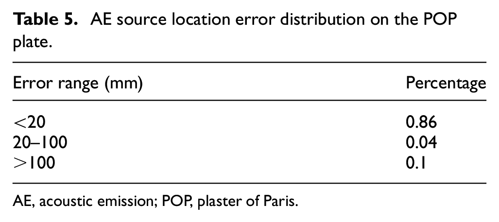
AE, acoustic emission; POP, plaster of Paris.

Source localisation for FP plate using 1D-CNN method: training stage

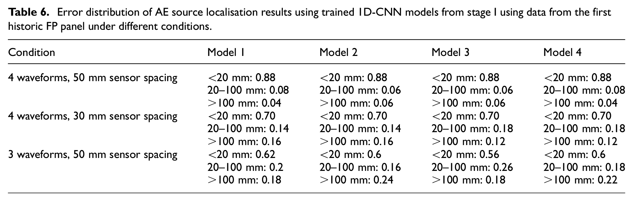
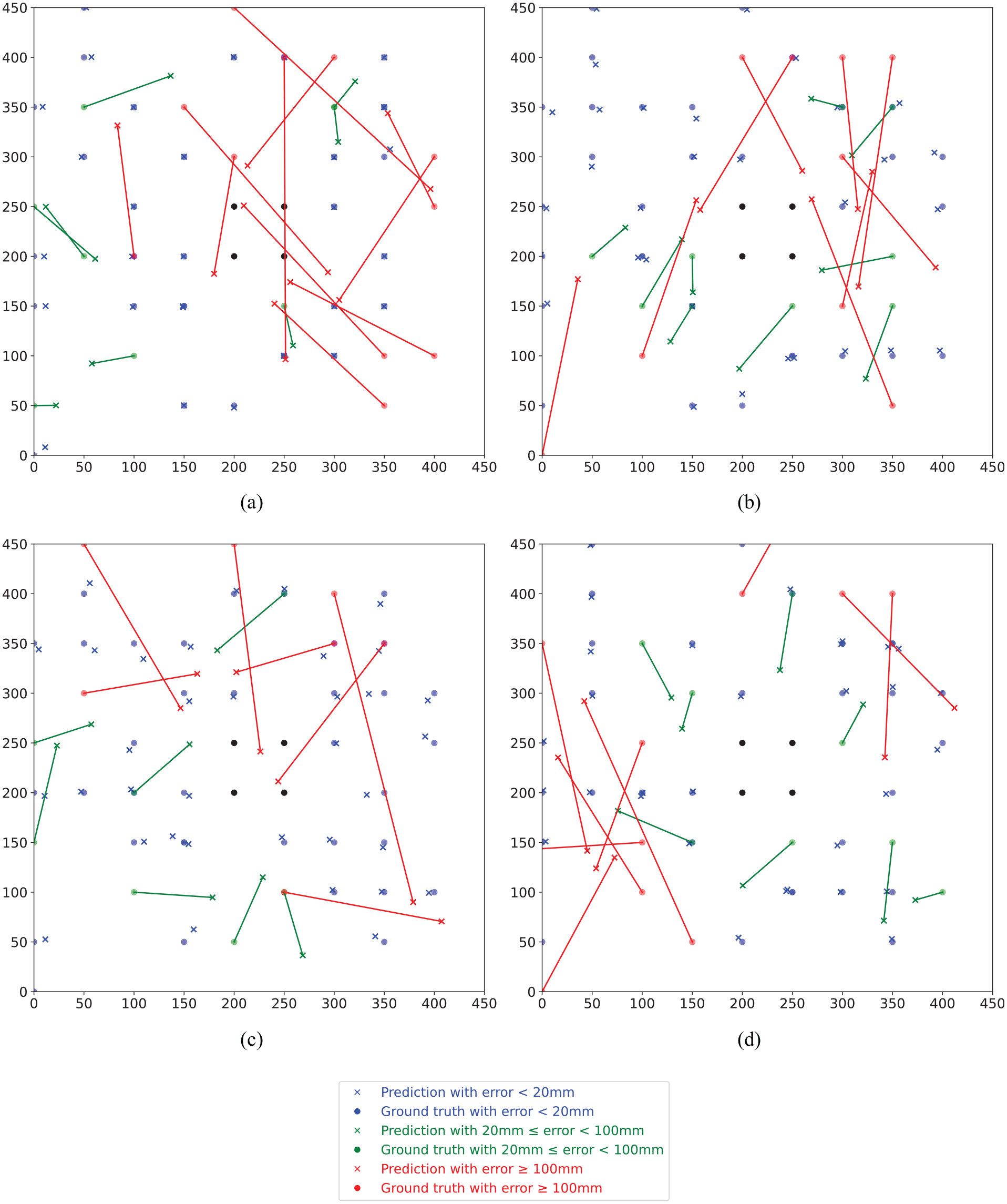
The results demonstrate the effectiveness of trained 1D-CNN models in AE source location estimation in FP plates. For the default configuration (i.e. four waveforms with a spacing of 50 mm), over 85% of the data had an error of estimation less than 20 mm, with only a few data points (<6%) predicted with an unacceptable error (>100 mm). The test results provided by all four trained 1D-CNN models at this stage are visualised in Figure 15. The corresponding error distributions are summarised in Table 6.

Figure 15.

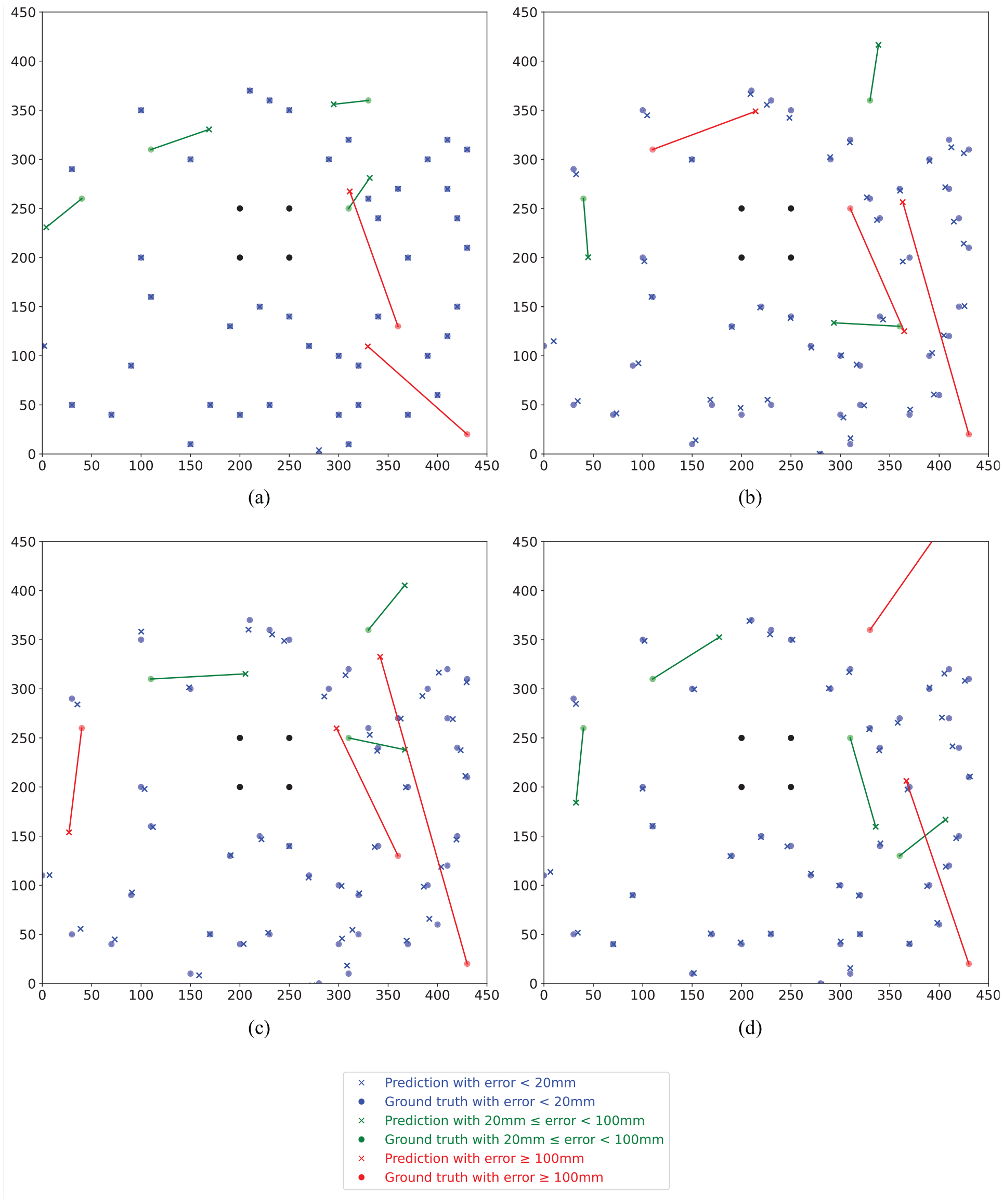
Source localisation results using the trained 1D-CNN models for the first historic FP panel (50 mm sensor spacing, 4 waveform signals): (a) model 1, (b) model 2, (c) model 3 and (d) model 4, axis labels in unit of mm.

Table 6.

Error distribution of AE source localisation results using trained 1D-CNN models from stage I using data from the first historic FP panel under different conditions.

Condition	Model 1	Model 2	Model 3	Model 4
4 waveforms, 50 mm sensor spacing	<20 mm: 0.88	<20 mm: 0.88	<20 mm: 0.88	<20 mm: 0.88
	20–100 mm: 0.08	20–100 mm: 0.06	20–100 mm: 0.06	20–100 mm: 0.08
	>100 mm: 0.04	>100 mm: 0.06	>100 mm: 0.06	>100 mm: 0.04
4 waveforms, 30 mm sensor spacing	<20 mm: 0.70	<20 mm: 0.70	<20 mm: 0.70	<20 mm: 0.70
	20–100 mm: 0.14	20–100 mm: 0.14	20–100 mm: 0.18	20–100 mm: 0.18
	>100 mm: 0.16	>100 mm: 0.16	>100 mm: 0.12	>100 mm: 0.12
3 waveforms, 50 mm sensor spacing	<20 mm: 0.62	<20 mm: 0.6	<20 mm: 0.56	<20 mm: 0.6
	20–100 mm: 0.2	20–100 mm: 0.16	20–100 mm: 0.26	20–100 mm: 0.18
	>100 mm: 0.18	>100 mm: 0.24	>100 mm: 0.18	>100 mm: 0.22

The subsequent test FP panel tests the source localisation performance of the trained 1D-CNN models on AE data from a different FP structure. The results showed that trained models used directly to estimate the source location can yield unacceptable accuracy, with only 20%–30% of the data having an error of estimation <20 mm, and most of the data estimated with large unacceptable errors exceeding 100 mm. For brevity, the results of this part are not shown. To overcome this issue, the approach of fine-tuning is applied to the trained models.

Source localisation for FP plate using 1D-CNN method: fine-tuning stage and ensemble learning stage

The AE source localisation results provided by the fine-tuned models for the default configuration on the subsequent test FP panel are shown in Figure 16, indicating a significant improvement in accuracy. The percentage of source location estimates with an error of less than 20mm has increased from 20%–30% to 60%–65%. However, despite the improvement, a considerable proportion of estimates (20%–30%) still have errors exceeding 100 mm, which is deemed unacceptable for real-world applications.

Figure 16.

Source localisation results using the fine-tuned 1D-CNN models for the subsequent test historic FP panel (50 mm sensor spacing, 4 waveform signals): (a) model 1-ft, (b) model 2-ft, (c) model 3-ft and (d) model 4-ft, axis labels in unit of mm.

To improve the accuracy of source localisation, the ensemble learning method is used, and its effectiveness is demonstrated through the final results for AE source localisation for the default configuration, as shown in Figure 17. An example demonstrating the process of combining four predictions into one is visualised in Figure 18. Two closest predicted coordinates are averaged to obtain the final prediction. The results reveal that the ensemble learning-based estimation significantly outperformed the independent fine-tuned model estimations. Specifically, the proportion of estimates with small errors (less than 20mm) improved considerably with values of 94%. The percentage of estimates with unacceptable errors reduced substantially to only 2%. The corresponding error distributions are summarised in Table 7.

Figure 17.

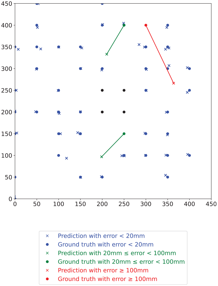
Source localisation results using the ensemble learning-based model for the subsequent test historic FP panel (50 mm sensor spacing, 4 waveform signals), axis labels in units of mm.

Figure 18.

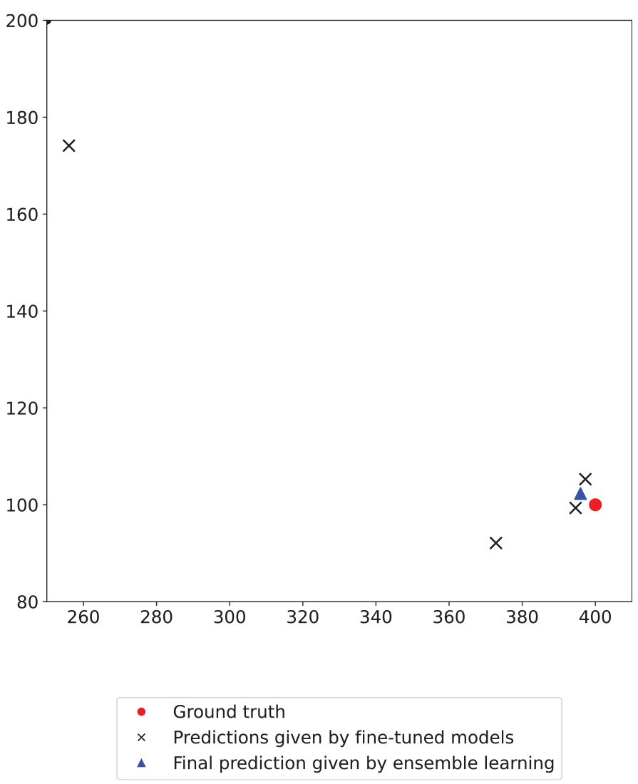
An example demonstrating the process of combining four predictions to one final prediction in stage III, axis labels in units of mm.

Table 7.

Error distribution of AE source localisation results using fine-tuned 1D-CNN models from stage II and ensemble learning method from stage III using data from the subsequent test historic FP panel under different conditions.

Condition	Model 1-ft	Model 2-ft	Model 3-ft	Model 4-ft	Ensemble learning-based model
4 waveforms, 50 mm sensor spacing	<20 mm: 0.62	<20 mm: 0.64	<20 mm: 0.72	<20 mm: 0.66	<20 mm: 0.94
	20–100 mm: 0.16	20–100 mm: 0.18	20–100 mm: 0.14	20–100 mm: 0.16	20–100 mm: 0.04
	>100 mm: 0.22	>100 mm: 0.18	>100 mm: 0.14	>100 mm: 0.18	>100 mm: 0.02
4 waveforms	<20 mm: 0.64	<20 mm: 0.7	<20 mm: 0.64	<20 mm: 0.62	<20 mm: 0.90
30 mm sensor spacing	20–100 mm: 0.16	20–100 mm: 0.08	20–100 mm: 0.08	20–100 mm: 0.1	20–100 mm: 0.04
30 mm sensor spacing	>100 mm: 0.2	>100 mm: 0.22	>100 mm: 0.28	>100 mm: 0.28	>100 mm: 0.06
3 waveforms, 50 mm sensor spacing	<20 mm: 0.62	<20 mm: 0.7	<20 mm: 0.62	<20 mm: 0.66	<20 mm: 0.88
	20–100 mm: 0.22	20–100 mm: 0.12	20–100 mm: 0.1	20–100 mm: 0.08	20–100 mm: 0.08
	>100 mm: 0.16	>100 mm: 0.18	>100 mm: 0.28	>100 mm: 0.26	>100 mm: 0.04

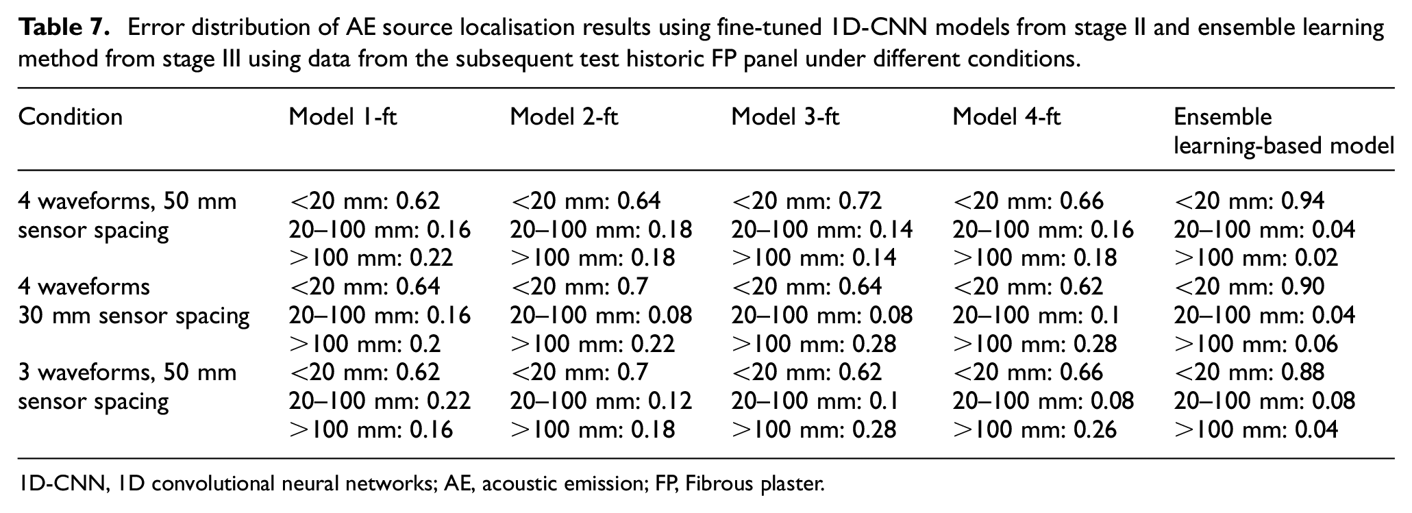
1D-CNN, 1D convolutional neural networks; AE, acoustic emission; FP, Fibrous plaster.

The study investigates two alternative ensemble learning methods: simple averaging and weighted averaging. The weights for the latter approach are determined based on the MSE of each fine-tuned model during its validation when the model converges during the fine-tuning training process. The results obtained indicate that, for simple averaging, there were 17 cases with errors falling within the 0–20 mm range (indicating high accuracy), 31 cases with errors between 20 and 100 mm (indicating acceptable accuracy), and 2 cases with errors exceeding 100 mm (indicating unacceptable accuracy). In the case of weighted averaging, there were 13 cases with errors within the 0–20 mm range (indicating high accuracy), 33 cases with errors between 20 and 100 mm (indicating acceptable accuracy), and 4 cases with errors exceeding 100 mm (indicating unacceptable accuracy). Comparing these accuracy metrics to the method described in the paper, it is evident that both simple and weighted averaging approaches exhibit lower accuracy than the partial averaging approach developed in this study.

The computation time required by the proposed three-stage 1D-CNN method can be broken down as follows: The first training phase, which uses a dataset of 172 sets of data, requires around 8–9 h. The fine-tuning phase, which uses a smaller dataset of 79 sets for each new area, takes about 20 minutes. The computer model utilised is a MacBook Pro equipped with a 2.3 GHz 8-Core Intel Core i9 processor (Intel Core i9-9880H, 9th Generation (Coffee Lake), 2.3 GHz base clock speed, up to 4.8 GHz Turbo Boost, 8 cores, 16 threads, 16 MB SmartCache, 45W TDP) and Intel UHD Graphics 630 1536 MB graphics (Intel UHD Graphics 630, 350 MHz base frequency, 1.20 GHz maximum dynamic frequency, 24 execution units, 4096 x 2304 @ 24Hz (HDMI 1.4), 5120 x 3200 @ 60Hz (DP), DirectX 12, OpenGL 4.5, 1536 MB shared memory).

These findings highlight the effectiveness of the ensemble learning approach in enhancing the accuracy of source localisation, especially in cases where individual fine-tuned models fail to provide accurate results. The low percentage of estimates with unacceptable errors indicates that the failure detection process will not be significant in practice. Overall, our study highlights the effectiveness of fine-tuning and ensemble learning in improving the accuracy of trained models in practical applications for the AE source localisation in historic FP ceilings.

Influence of sensor spacing and waveform number in 1D-CNN-based method

The AE source localisation results for configuration (b) (four sensors with 30 mm spacing) and configuration (c) (three sensors with 50 mm spacing) were also examined using the three-stage approach. The error distribution histogram of source localisation results using ensemble learning method for the subsequent test historic FP panel using the three configurations is shown in Figure 19. Tables 6 and 7 summarise the error distributions for the trained models during the training stage and the fine-tuning and ensemble learning stages.

Figure 19.

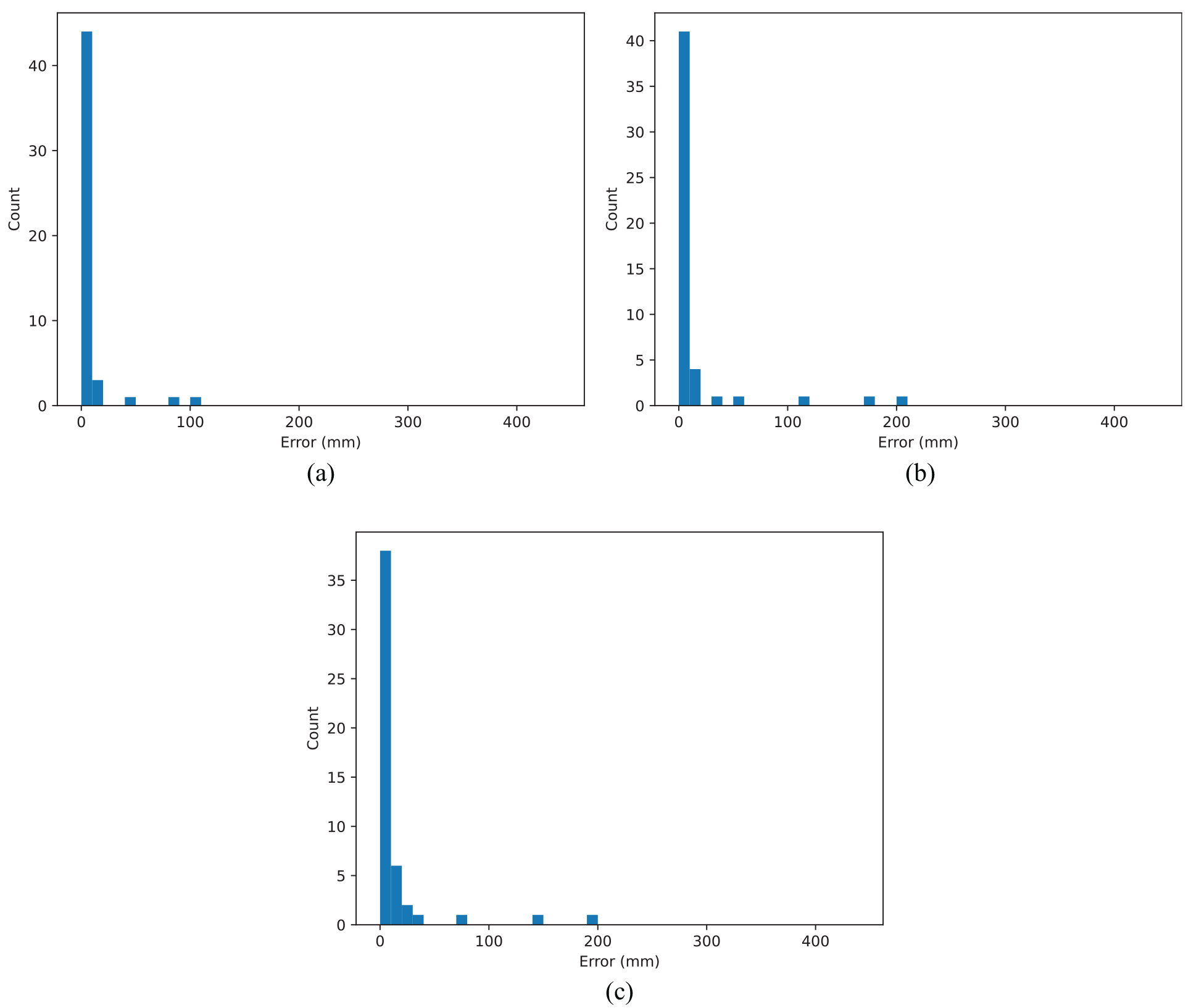
Error distribution histogram of source localisation results using ensemble learning method for the subsequent test historic FP panel using (a) configuration, (b) configuration and (c) configuration.

The results indicate that configuration (b) had 90% of estimates with errors less than 20 mm and 6% of estimates with errors exceeding 100 mm, demonstrating that the sensor spacing had minimal effect on the AE source localisation performance provided by the proposed three-stage approach in configuration (b).

For configuration (c), the proposed three-stage approach was also found to be effective but with a slightly deteriorated accuracy, with 88% of estimates having small errors and only 4% of estimates having errors exceeding 100 mm. Although the high accuracy percentage of this configuration is 6% lower than the default configuration, the unacceptable error remains within acceptable limits. Thus, the results suggest that sufficient localisation can still be achieved with three sensors.

Source localisation results by TDOA-based beamforming method using sensor cluster

The developed three-stage 1D-CNN method was evaluated by comparing its performance to that of the TDOA-based beamforming method. An example of the estimated incidence angles can be seen in Figure 20.

Figure 20.

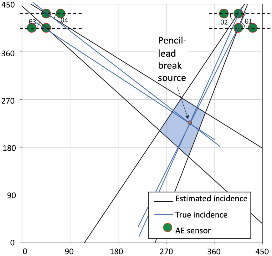
Source localisation results using the TDOA-based beamforming method with two Z-shaped sensor clusters with the estimated incidence angles, $θ_{1}$ and $θ_{2}$ , $θ_{3}$ and $θ_{4}$ , axis labels in units of mm.

It can be observed that there is a significant deviation between the estimated incidence angles and the true incidence angles (connecting the source with the sensor cluster). The angle estimation error for the historical FP ceiling panel ranges from 20° to 40°. Even with two sensor clusters, it is not possible to achieve consistently high accuracy results. The blue area visualises the area where AE source may be predicted with the beamforming method. To experimentally compare measurement accuracy of the developed technique with the beamforming method, 20 pencil-lead breaks were produced at random positions within the (0, 450) range for both x and y coordinates. The coordinates were predicted using the sensor setup shown in Figure 20. The resulting average maximum distance between the actual and predicted coordinates within this area is 71 mm, with a standard deviation of 20.8 mm. This is primarily due to inaccurate identification of the TDOA which is complicated by uncertainties arising from the anisotropic structure of the test object and the attenuation of the received AE signal. In contrast, when utilising the proposed 1D-CNN-based method to predict the 50 pencil-lead break sources in the test dataset, the average error distance between the predictions and the ground truth is 4.07 mm, with a standard deviation of 2.84 mm.

This result highlights several limitations of this method in the damage source localisation for historic FP ceilings. Firstly, the accurate extraction of the first arrival wave is critical but relies on an empirical approach that can impact the localisation accuracy. Secondly, the method requires a minimum of six sensors to form two L-shaped clusters that are positioned far apart, increasing the hardware cost. In contrast, the method proposed in this manuscript, based on 1D-CNN, achieves accurate damage source localisation using only four sensors. This distinction highlights the efficient and cost-effective nature of the 1D-CNN-based method introduced in this paper.

Conclusion

The AE source localisation in anisotropic plate-like structures has long been recognised as a complex problem. This article addresses the limitations of the TDOA method using the beamforming technique, which is a commonly used approach for AE source localisation. To overcome these limitations, we propose a new technique. We applied this technique to historic FP ceiling panels, which are heterogenous and anisotropic. In our experimental setup, sensors are placed in a square-shaped cluster and collect signals produced by the pencil-lead breaking source. A three-stage approach was then adopted to process the data, where four 1D-CNN models with different dropout layer implementations were trained and validated to localise the pencil-break. These models were then fine-tuned to estimate the source location of a new FP panel. The ultimate estimation results from the combination of estimations provided by the four distinct fine-tuned models. The results of the experiments demonstrate that the 1D-CNN method developed in this study can provide highly accurate localisation, where up to 94% of location predictions are accurate to 20 mm. Adopting different sensor spacing or reducing the number of sensors from four to three sensors instead of four) does not significantly influence localisation accuracy.

Furthermore, the three-stage approach using 1D-CNN models shows superior accuracy and versatility in AE source localisation for historic FP panels, compared to the existing TDOA-based method using sensor clusters, with fast fine-tuning, automation and the ability to work with fewer sensors. Results suggest that the 1D-CNN model can be a promising method for detecting the failure source of historic FP ceilings. The localisation approach developed in this paper can also be applied to other anisotropic plate-like structures.

Footnotes

Declaration of conflicting interests

The author(s) declared no potential conflicts of interest with respect to the research, authorship, and/or publication of this article.

Funding

The author(s) disclosed receipt of the following financial support for the research, authorship, and/or publication of this article: The authors would like to acknowledge the generous support of the ICE research and development enabling fund in the development and presentation of this research.

ORCID iD

Jiaxu Zuo

References

Ngah

Dams

Ansell

, et al. Structural performance of fibrous plaster. Part 1: physical and mechanical properties of hessian and glass fibre reinforced gypsum composites. Constr Building Mater 2020; 259: 120396.

Zuo

Mayfield

Ozdemir

, et al. Preliminary experimental investigation on mechanical properties of historic fibrous plaster. In: Paper presented at SAHC2023: 13th International conference on structural analysis of historic constructions, 2023.

Historic England. Historic Fibrous Plaster in the UK: Guidance on its Care and Management. Swindon. Historic England, 2019.

Gopinath

Ramadoss

. Review on structural health monitoring for restoration of heritage buildings. Mat Today Proc 2021; 43: 1534–1538.

Chandarana

Sanchez

Soutis

, et al. Early damage detection in composites during fabrication and mechanical testing. Materials 2017; 10: 685.

Sause

Müller

Horoschenkoff

, et al. Quantification of failure mechanisms in mode-I loading of fiber reinforced plastics utilizing acoustic emission analysis. Compos Sci Technol 2012; 72: 167–174.

Zhou

Mathews

Adams

. Acoustic emission–based impact location estimation on composite structures. Struct Health Monit 2019; 18: 1652–1668.

Zhou

Pan

Wang

, et al. Review on acoustic emission source location, damage recognition and lifetime prediction of fiber-reinforced composites. Journal of Materials Science. 2023; 58(2): 5837–607.

Gangadharan

Prasanna

Bhat

, et al. Acoustic emission source location in composite structure by Voronoi construction using geodesic curve evolution. J Acoust Soc Am 2009; 126: 2324–2330.

10.

Romhany

Czigany

Karger-Kocsis

. Failure assessment and evaluation of damage development and crack growth in polymer composites via localisation of acoustic emission events: a review. Polymer Rev 2017; 57: 397–439.

11.

Dong

Zou

Sun

, et al. Some developments and new insights for microseismic/acoustic emission source localisation. Shock Vibr. Epub ahead of print 22 July 2019. DOI: 10.1155/2019/9732606.

12.

Kundu

Nakatani

Takeda

. Acoustic source localisation in anisotropic plates. Ultrasonics 2012; 52: 740–746.

13.

Xiao

Pan

, et al. A novel acoustic emission beamforming method with two uniform linear arrays on plate-like structures. Ultrasonics 2014; 54: 737–745.

14.

Sen

Gawronski

Packo

, et al. Square-shaped sensor clusters for acoustic source localisation in anisotropic plates by wave front shape-based approach. Mech Syst Signal Process 2021; 153: 107489.

15.

Park

Packo

Kundu

. Acoustic source localisation in an anisotropic plate without knowing its material properties – a new approach. Ultrasonics 2017; 79: 9–17.

16.

Aljets

Chong

Wilcox

, et al. Acoustic emission source location in plate-like structures using a closely arranged triangular sensor array. J Acoust Emission 2010; 28: 85–98.

17.

Aljets

Chong

Wilcox

, et al. Acoustic emission source location on large plate-like structures using a local triangular sensor array. Mech Syst Signal Proc 2012; 30: 91–102.

18.

Sen

Kundu

. Acoustic source localisation in a highly anisotropic plate with unknown orientation of its axes of symmetry and material properties with numerical verification. Ultrasonics, 2020; 100: 105977.

19.

Yin

Cui

Kundu

. Acoustic source localisation in anisotropic plates with “Z” shaped sensor clusters. Ultrasonics 2018; 84: 34–37.

20.

Nakatani

Kundu

Takeda

. Improving accuracy of acoustic source localisation in anisotropic plates. Ultrasonics, 2014; 54: 1776–1788.

21.

De Simone

Ciampa

Boccardi

, et al. Impact source localisation in aerospace composite structures. Smart Mater Struct 2017; 26: 125026.

22.

Sen

Kundu

. A new wave front shape-based approach for acoustic source localisation in an anisotropic plate without knowing its material properties. Ultrasonics 2018; 87, 20–32.

23.

Sen

Kundu

. Acoustic source localisation in a highly anisotropic plate with unknown orientation of its axes of symmetry and material properties with numerical verification. Ultrasonics 2020; 100: 105977.

24.

Kalafat

Sause

MGR

. Acoustic emission source localisation by artificial neural networks. Struct Health Monit 2015; 14: 633–647.

25.

Sause

MGR

Schmitt

Hoeck

, et al. Acoustic emission based prediction of local stress exposure. Compos Sci Technol 2019; 173: 90–98.

26.

Ding

Xiu

Wan

, et al. Location of tensile damage source of carbon fiber braided composites based on two-step method. Molecules 2019; 24: 3524.

27.

Zhang

Liu

, et al. Development of an artificial neural network for source localisation using a fiber optic acoustic emission sensor array. Struct Health Monit 2015; 14: 168–177.

28.

Zhang

Wang

Hou

, et al. 1D-CNN-based damage identification method based on piezoelectric impedance using adjustable inductive shunt circuitry for data enrichment. Struct Health Monit 2022; 21: 1992–2009.

A three-stage approach based on 1D-CNNs for AE source localisation on historic fibrous plaster ceilings

Abstract

Keywords

Introduction

Methodology

Data acquisition system and test configuration

AE signal processing

CNN architecture and implementation details

CNN architecture

Dropout layer implementation

D-CNN models

Stage I: Training stage

Stage II: Fine-tuning

Stage III: ensemble learning

Experiment

Test objects

Experimental setup

Accuracy of recorded source locations

Uncertainties

Accuracy thresholds for AE source localisation by 1D-CNNs

Results and discussion

Source localisation results on POP plate using 1D-CNN

Source localisation for FP plate using 1D-CNN method: training stage

Source localisation for FP plate using 1D-CNN method: fine-tuning stage and ensemble learning stage

Influence of sensor spacing and waveform number in 1D-CNN-based method

Source localisation results by TDOA-based beamforming method using sensor cluster

Conclusion

Footnotes

Declaration of conflicting interests

Funding

ORCID iD

References